Is There a Purchase Limit on Regional Growth? A Quasi-experimental Evaluation of Investment Grants Using Matching Techniques

Abstract

In this article, we apply recent advances in quasi-experimental estimation methods to analyze the effectiveness of Germany’s large-scale regional policy instrument, the joint Federal Government/State Programme “Gemeinschaftsaufgabe Verbesserung der regionalen Wirtschaftsstruktur” (GRW), which is a means to foster labor-productivity growth in lagging regions. In particular, adopting binary and generalized propensity-score matching methods, our results indicate that the GRW can be generally considered effective. However, we find evidence for a nonlinear relationship between GRW funding and regional growth associated with a maximum subsidy level beyond which financial support does not generate further labor-productivity growth. In other words, there is a “purchase limit” on regional growth. Although the matching approach is very appealing due to its methodological rigor and didactical clarity, throughout the empirical application, we faced difficulties in balancing the set of covariates among treated and comparison regions, given that two sets of the regions differ strongly with respect to their underlying structural characteristics. Such imperfect balancing may limit the practical applicability of matching techniques in regional data settings. Overall, however, the matching approach can still be considered of great value for regional policy analysis and should be the subject of future research efforts in the field of empirical regional science.

Keywords

quasi-experimental control group estimation generalized propensity score matching labor productivity growth regional policy

Introduction

Recent advances in applied econometrics have revolutionized the way economists and allied social scientists have addressed the issue of causality when confronted with observational data (i.e., data that do not come from a randomized controlled trial). Angrist and Pischke (2010) call this the “credibility revolution” in empirical economics.¹ While much of the previous work concerned with econometric evaluation involved a structural modeling framework, current applied work is dominated by the “experimentalist” school of thought, where emphasis is on credibly estimating a particular causal parameter of interest, sometimes even in the absence of an explicit structural model.² When quasi-experimental evaluation methods³ can be properly applied, this approach has the potential to give us reliable estimates of “treatment effects” (Wooldridge 2010) without an appeal to the sometimes very strong assumptions that underlie much of structural work.

Given that quasi-experimental evaluation methods have started to attract more attention in regional science, in the following, we give a brief overview of recent innovations in the field and apply matching estimation—one of the prominent tools of the experimentalist school—to study the effect of regional policy measures on economic growth. More explicitly, we estimate the causal effect of private sector investment subsidies and business-related infrastructure measures in Germany under the umbrella of the “Gemeinschaftsaufgabe Verbesserung der regionalen Wirtschaftsstruktur” (GRW) on labor-productivity growth for German Nomenclature of Territorial Units for Statistics (NUTS) 3 districts. The GRW is arguably the most powerful instrument of German regional policy (Alecke, Mitze, and Untiedt 2013). Since the reunification of West and East Germany, more than €60 billion has been spent to foster regional growth in structurally weak regions. The GRW also includes European Union (EU) regional policy grants by means of the European Regional Development Fund (ERDF).

In the present article, the estimation of the general effectiveness of German regional policy is done by means of two complementary quasi-experimental control group approaches. First, we use a binary treatment indicator related to the policy status and apply propensity-score-based matching to compare the growth performance of GRW-funded and non-funded regions. This empirical identification strategy allows us to answer the question of whether the receipt of a subsidy boosts regional growth at all. Second, we calculate—for the subgroup of funded regions—the range at which regional support is able to induce higher growth using a generalized propensity-score (GPS) approach (Hirano and Imbens 2004) for a continuous treatment indicator (i.e., the amount of subsidy). This latter identification strategy is able to give an estimate of up to what extent a higher subsidy level is associated with a better growth performance. Figure 1 provides a graphical presentation of our empirical evaluation strategy based on the two complementary quasi-experimental control group approaches.

Figure 1.

Graphical overview of empirical evaluation strategy.

Our result suggests that GRW-funded regions indeed experienced higher labor-productivity growth compared to non-funded regions, indicating that the GRW is generally effective in balancing standards of living among German regions. However, the relationship between GRW funding and regional growth is nonlinear. We find that up to a funding intensity which corresponds to the 67th percentile of the regional distribution of GRW payments—or roughly €105,000 of GRW payments per labor force—higher subsidies ensure higher productivity growth. Thereafter, more funding does not necessarily induce increased growth. Likewise, a minimum funding intensity is needed in order to generate positive growth effects for our sample of German NUTS3 regions.

Thus, in line with earlier work on EU regional funding by Becker et al. (2012), we provide empirical evidence for a maximum desired subsidy level after which a further policy stimulus does not have any positive effect on the regional economic performance. This finding may be seen as an extension to earlier work such as in Alecke, Mitze, and Untiedt (2013), who find a positive policy effect of the GRW on regional productivity using a linear regression approach. Similar results were also reported in earlier studies by Röhl and von Speicher (2009) as well as Schalk and Untiedt (2000), among others. However, these studies typically focus on the average effect of GRW funding on regional economic growth without identifying the range of funding intensities for which the policy support is effective.

Although the quasi-experimental approach is very appealing from a methodological and didactic perspective, applications to regional data have to be interpreted with some caution. This is due to the fact that regional data are associated with special features that are likely to complicate empirical applications, particularly in terms of satisfying the so-called balancing property. In other words, for a finite sample of regional observations, it is very hard to find perfect statistical twins in order to make sensible comparisons of mean outcomes. Moreover, the crucial assumption of “no general-equilibrium effects” (i.e., the stable unit treatment value assumption or SUTVA) is difficult to justify in a regional setting. Thus, another contribution of our article is to demonstrate the hurdles in directly applying methods largely developed in another field of economics to study circumstances that are of interest to regional scientists.

Methodological Approaches in Regional Science and Policy Analysis

We take the current topology of the literature as given—that is, whether economists ought to be doing structural or experimental work is not within the scope of this article.⁴ More modestly, our aim is to demonstrate that some of the non- and quasi-experimental methods primarily developed by labor economists have applicability in regional studies as well, but that the nature of regional data presents some difficulties that are not typically encountered in individual-level studies common in applied labor microeconometrics. Macroeconomics and industrial organization, both of which heavily influence the methods used in regional science, have not followed the experimentalist revolution in labor economics. By implication, regional studies has not fully benefited from the so-called credibility revolution, particularly its emphasis on identification of causal parameters of interest.

The question of whether more experimental studies should be done in regional science and policy analysis is something else. Clearly, the choice of the right method for empirical analyses is a crucial factor since—as Bartels (1982) points out—the social relevance of regional science research is very much determined by the quality of regional policy analysis. Holmes (2010) has delineated the existing approaches in regional science and policy analysis into three types: descriptive, experimentalist, and structural. As can be reasonably expected from a regional scientist, he seems to be more sympathetic to the structural approach, noting that analyses of this type have been successfully applied in industrial organization, which in turn has a leading influence on regional science. Nevertheless, he is not entirely dismissive of the experimentalist method. He correctly notes that this approach has encouraged researchers to think about causation more carefully. Descriptive studies which are prevalent in the regional studies literature now suffer from diminished credibility as a result of the emphasis of the experimentalist school of thought on the sanctity of the identification strategy.⁵

As Feser (2013) shows in a comprehensive literature survey, the introduction of quasi-experimental control group designs for the evaluation of regional policies can be dated back to the seminal contribution of Isserman and Merrifield (1982). Recently, regional scientists have also started to consequently accommodate some of the methodical advances of the experimentalist school, such as the use of regression discontinuity or matching estimation. For instance, Billings (2009) uses administrative regional borders to analyze the effect of geographical differences in tax credits on the formation of new businesses, and Dell (2010) employs discontinuities in Peru’s regions to examine the effect of historical institutions on economic development.⁶ Closely related to the scope of this article, Becker et al. (2010) apply a regression discontinuity design to examine the effectiveness of EU regional policy. The authors make use of the institutional design of the EU objective 1 subsidy scheme, which qualifies regions for structural funds payments if they have a per capita gross domestic product (GDP) level below 75 percent of the EU average. Using this threshold, the authors exploit the discrete jump in the probability of EU transfer receipt for their empirical identification strategy and find that objective 1 payments have a positive impact on GDP growth.

Becker et al. (2012) and Mohl and Hagen (2008) examine the impact of EU structural funds on regional growth by means of matching methods. The fundamental idea underlying the matching approach is to construct a counterfactual situation which is able to answer the question, “What would have happened to the regional growth paths of two regions if everything else is equal in these regions except that one region did receive funding while the other did not?” The latter situation calls for a binary subsidy–receipt indicator that splits regional entities into subsidized and nonsubsidized (comparison) regions. In the case of a continuous subsidy-level variable, one could ask, “What would have happened to the regional growth paths if everything else is equal except that one region received a higher (lower) level of funding compared to the other?” Thus, the single most important task in matching estimation, as implied by its name, is to find “statistical twins” which only differ by subsidy status and no other structural characteristics that might impact on the observed economic growth performance.

A Framework for Evaluating Regional Policies

Causal Inference and the Potential-outcome Model

In this section, we briefly describe the underlying formal framework of much of the experimental or quasi-experimental techniques used for causal inference. This is based on the so-called potential-outcome model developed in the statistics literature by Neyman as early as 1923 [1990].

Suppose we have a sample of N individual observations (say, regions) denoted by i and there are only two time periods (pre- and posttreatment). Our response variable is y_i (say, labor-productivity growth) and a treatment indicator, d_i , equals 1 if i received the treatment (i.e., a regional subsidy) and 0 otherwise. Before treatment is administered, two potential outcomes exist, y_i (0) and y_i (1), which represent outcomes if i did not or did receive the treatment, respectively.

After the receipt of the subsidy, we only observe $y_{i} = y_{i} (d_{i}) = y_{i} (0) (1 - d_{i}) + y_{i} (1) (d_{i})$ . For a particular region, we cannot observe the gross grain or loss, $y_{i} (1) - y_{i} (0)$ , because both outcomes cannot be observed simultaneously. This represents the “fundamental problem of causal inference” (Holland 1986). In terms of average effects, this implies the following:

τ_{A T E} = E [y_{i} (1) - y_{i} (0)],

τ_{A T E T} = E [y_{i} (1) - y_{i} (0) | d_{i} = 1],

where ATE and ATET refer to the average treatment effect and average treatment effect on the treated, respectively. The goal is to recover these average effects by estimating the counterfactual situation.

One has to note that the individual observations are characteristically different from each other in important dimensions that affect both the probability of receiving a certain amount of treatment and the response variable. Without taking this into account, a simple comparison of mean outcomes at different treatment intensities (i.e., levels of funding) is unable to provide us with a consistent estimate of the treatment effect (i.e., the effect of a particular level of funding on economic growth) because of the selection-into-treatment bias:

\begin{aligned} E [y_{i} | d_{i} = 1] - E [y_{i} | d_{i} = 0] & = \{E [y_{i} (1) | d_{i} = 1] - E [y_{i} (0) | d_{i} = 1]\} \\ + {E [y_{i} (0) | d_{i} = 1] - E [y_{i} (0) | d_{i} = 0]} . \end{aligned}

The equation above shows that the observed difference can be decomposed into two parts. One is the ATET since $E [y_{i} (1) | d_{i} = 1] - E [y_{i} (0) | d_{i} = 1]$ is equal to $E [y_{i} (1) - y_{i} (0) | d_{i} = 1]$ . This is equal to the observed difference only when the second component, $E [y_{i} (0) | d_{i} = 1] - E [y_{i} (0) | d_{i} = 0]$ , which represents the selection bias, is equal to zero.

The selection bias might manifest itself in this particular case of regional policy evaluation by virtue of the fact that underperforming regions are precisely the ones that are given the subsidy. In other words, the recipients of the treatment are characteristically different from the nonrecipients, and these characteristics are most likely correlated with the response variable of interest. In this case, ordinary regression estimates that do not take these differences into account are likely biased and inconsistent, and, therefore, are of very little use for evaluating the effectiveness of the policy.

The Matching Approach

One way to address this evaluation problem is to employ a matching approach based on the GPS to eliminate biases generated by the inherent differences between regions as captured by the covariates (Hirano and Imbens 2004). This approach is a generalized version of conventional propensity-score matching (Rosenbaum and Rubin 1983) in that matching on the GPS allows for the continuous (as opposed to binary) nature of the treatment variable.⁷ In this article, we address the problem of regional policy evaluation in two steps: first, we use a binary treatment indicator; and second, we take into account the intensity of treatment.

Before we describe matching on the GPS, we begin with the simpler case of a binary treatment to illustrate the mechanics of matching methods. The basic idea underlying the matching approach is to obtain a statistical twin of a treated region but which comes from the untreated group. Under fairly mild assumptions, the mean of the differences in outcomes between treated and untreated regions represents an estimate of the policy effect (Rosenbaum and Rubin 1983). For a specific matched pair, the outcome for the untreated labor-market region is therefore construed as the counterfactual situation for the treated region—that is, it represents economic growth in a region which received funding had that particular region not, in fact, receive funding.⁸

What is essential for matching methods to generate consistent estimates is for the assumption of conditional independence to hold:

(y_{i} (1), y_{i} (0)) ⊥ d_{i} | x_{i},

where

⊥

denotes statistical independence and x _i is a vector of covariates; i indexes units of observation. This implies that, although regions may differ in their observed characteristics x _i , adjusting for these observable characteristics eliminates the biases associated with them. Thus, the conditional-independence assumption (CIA) is equivalently formulated as:

Pr (d_{i} = 1 | y_{i} (1), y_{i} (0), x_{i}) = P r (d_{i} | x_{i}),

where

P r (d_{i} = 1 | x_{i})

is called the propensity score, that is, the probability of treatment receipt. Notably, this equation precludes any “selection on unobservables,” that is, the covariates x _i capture all factors that determine the treatment probability.

Rosenbaum and Rubin (1983) show that when the CIA holds, then it is also true that $(y_{i} (1), y_{i} (0)) ⊥ d_{i} | P r (d_{i} = 1 | x_{i})$ .⁹ This important result states that if conditioning on the covariates x _i eliminates the selection bias, then conditioning on the propensity score can just as well do the same.

The level of potential subsidy is a continuous variable: $γ \in [γ_{0}, γ_{1}]$ . In this case, it is more appropriate to use the GPS, so we can calculate the dose–response function, that is, the treatment effect at every level of the subsidy. Following Hirano and Imbens (2004) and Bia and Mattei (2008), define the potential outcomes as $y_{i} (γ)$ and maintain that CIA holds: $y_{i} (γ) ⊥ g_{i} | x_{i}$ , where g_i is the actual subsidy received. We assume that this condition—called weak unconfoundedness—holds for all $γ \in G = [γ_{0}, γ_{1}]$ . The fundamental problem of causal inference remains since we are only able to observe the triple ${x_{i}, g_{i}, y_{i} (γ = g_{i})}$ once the subsidy is supplied; the entire set of potential outcomes $y_{i} (γ)$ remains unknown.

The GPS is defined as $s_{i} \equiv ω ({g_{i}, x}_{i})$ , where $ω (γ, x)$ is the conditional density of the treatment variable given the covariates. An important result derived by Hirano and Imbens (2004) is that weak unconfoundedness given the GPS is equivalent to weak unconfoundedness given the covariates:

y_{i} (γ) ⊥ g_{i} | s_{i} \forall g_{i} \in γ .

Therefore, the GPS has the same bias-elimination property in the continuous treatment case as that demonstrated by the propensity score in the case of binary treatments.

To assess the quality of the matching procedure, researchers typically test whether the treatment and comparison groups are balanced. Caliendo and Kopeinig (2008) list a few methods to evaluate covariate balance: the use of the standardized bias (SB), a t-test, a test using the pseudo R ², a test for joint significance (Sianesi 2004), and a stratification test based on Dehejia and Wahba (1999, 2002). The basic idea behind these approaches is to check whether systematic differences between treatment and control groups remain even after conditioning on the propensity score.

Analyzing the sensitivity of the estimation results is another important feature in applied work (Caliendo and Kopeinig 2008). A focal point here is to test for the potential role of hidden biases stemming from unobserved variables that influence the probability of receiving treatment. A prominent test to quantify this source of bias is to calculate Rosenbaum (2002) bounds. As DiPrete and Gangl (2004) point out, the Rosenbaum bounding approach can be interpreted as a worst-case scenario to test for the stability of the estimated outcome differences between treated and nontreated individuals given the existence of unobserved influencing factors. Rosenbaum bounds then quantify what the necessary strength of an unmeasured influence has to be in order to significantly impact the estimated ATET operating through selection effects.

Empirical Application: Data and Estimation Results

The GRW is the most important regional policy instrument in Germany and operates as a coordinated policy between the German federal government, the state-level governments, and the EU’s ERDF. The goal of the GRW is to provide subsidies for investments of the private business sector in economically underdeveloped regions as well as the provision of business-related public infrastructure.¹⁰ Since the German reunification, roughly €61 billion has been spent to foster the equalization of living standards in the different regions of Germany, with a large part of the subsidy allocated to the East German recovery. About two-thirds of the overall funding volume was assigned to private sector investment subsidies (€39 billion).

We use annual data for the period 1993–2008 allocated to the 413 NUTS 3 districts in Germany in order to assess the effectiveness of the GRW. Descriptive statistics of the variables used throughout the empirical exercise are given in the Appendix. The response variable is the growth rate in labor productivity defined as the annual growth rate of GDP per worker. In the first step, our binary subsidy–receipt indicator takes the value of 1 if a region received GRW payments for at least one year in the period 1993–2008 and is 0 otherwise.

To estimate the propensity score (i.e., the probability of receiving a subsidy) for each region, we use a probit specification that models the receipt of GRW as a function of the following control variables: (1) the initial income gap in 1992 relative to the maximum income level observed in the sample period (as a proxy for steady-state income), (2) the average firm size defined as the number of workers per firm in each region, (3) the regional share of manufacturing sector employment in total regional employment, (4) the region’s human-capital endowment, (5) the population density defined as the population per area, as well as two dummy variables indicating, (6) whether the region is an independent urban municipality (kreisfreie Stadt) with more than 100,000 inhabitants or belongs to a greater administrative district otherwise (Landkreis), and finally (7) an ordinal variable based on a classification of the regional settlement structure, which takes values from 1 (center of an agglomerated area) to 9 (rural area in periphery).¹¹

The control variables were selected based on theoretical reasons and underlying institutional facts of the GRW instrument. For instance, the inclusion of the initial gap in labor-productivity levels in 1992 is supposed to capture the institutional features of the GRW scheme, which assigns regions as eligible for funding if they are classified as “structurally weak” by means of a composite indicator using different socioeconomic criteria (including historical and projected data on unemployment rates, income levels, infrastructure equipment, etc.).¹² Though the GRW thus does not have a strict linear relationship with relative productivity levels as compared to the institutional setting of the EU structural funds, relative income gaps may be seen as a key indicator which is highly correlated with other socioeconomic criteria such as unemployment rates.

Likewise, the average firm size and the regional employment share of manufacturing sectors serve as empirical proxies for the underlying regional business structure, which are likely to influence the probability of receiving GRW funding as well. Finally, human-capital endowment, population density, and the included indicator variables mark further transmission channels that are theoretically expected to affect the receipt of GRW grants by regions. Thus, our approach does not aim at replicating the classification scheme of the GRW, but rather makes use of a portfolio of regional characteristics in order to find proper comparison regions for our subsidized group that justifies the CIA.

We estimate the probit model of GRW receipt both in cross-sectional settings averaged over different time spans (1994–1998, 1998–2002, and 2000–2004) and for a pooled specification, which makes use of three-year averages in the entire interval 1993–2008.¹³ The motivation for the design of different subsamples is twofold. First, we want to quantify the effectiveness of GRW for different time periods. Second, we synthetically define pre-subsidy periods and control for pre-subsidy difference among the regions’ initial position in order to exclude feedback effects throughout the matching approach. This procedure is important for the success of the matching approach in terms of excluding any simultaneity bias stemming from feedback effects of the output variable on the subsidy-receipt indicator and the vector of conditioning factors x _i . The use of a further pooled specification can particularly be motivated by the gain in degrees of freedom for statistical inference associated with a richer set of information compared to the computation of cross-sectional averages. Also, by doing so, we can circumvent the ad hoc classification of synthetic pre-subsidy periods given that the GRW policy is in fact an on-going measure during our period of analysis. This may serve as an important sensitivity check for the cross-sectional estimates. To control for macroeconomic shifts throughout the sample period, we include time-fixed effects in the pooled estimation approach.

Estimation results for the alternative sample periods are shown in Table 1. Consistent with our theoretical expectations, the initial (logged) productivity gap is statistically significant and positively correlated with the probability of GRW receipt. The same holds for the average firm size. In contrast, the share of manufacturing sector employment in total regional employment and the regional human-capital endowment show negative coefficient signs. The negative correlation of the latter variables can be explained with regard to the specific situation of supported regions in East Germany. On one hand, these regions are still characterized by a large fraction of employees with a high level of formal education. On the other hand, these regions have also faced severe structural breaks in terms of transforming and deindustrializing their local economies in the aftermath of German reunification. As a result of this “unification shock”, East German regions experienced a strong decline in manufacturing sector activity and still show, on average, a low level of industrial concentration compared to the West German average. At the same time, they receive large amounts of GRW support, which drives the observed negative correlation between GRW funding and the share of manufacturing sector employment in total regional employment.

Table 1.

Propensity-Score (PS) Estimation for GRW Receipt (Probit Specification).

Subsidy (0/1): Receipt of GRW Funding	Cross Section	Cross Section	Cross Section	Pooled
Subsidy (0/1): Receipt of GRW Funding	1994–1998	1998–2002	2000–2004	1993–2008
Log (initial income gap)	1.452***	1.823***	2.425***	2.085***
SE	(0.2428)	(0.2518)	(0.3024)	(0.1235)
Log (average firm size)	1.325***	1.244***	0.559*	0.733***
SE	(0.2897)	(0.2981)	(0.3110)	(0.1335)
Log (share manufacturing sector)	−1.684***	−1.482***	−1.093***	−1.245***
SE	(0.2758)	(0.2747)	(0.2809)	(0.1212)
Log (human capital)	−0.892***	−0.761***	−0.398	−0.491***
SE	(0.2585)	(0.2636)	(0.2812)	(0.1206)
Log (population density)	−0.192	−0.118	−0.166	−0.088*
SE	(0.1222)	(0.1166)	(0.1286)	(0.0472)
Urban municipality indicator	−0.232	−0.280	−0.569*	−0.286**
SE	(0.2874)	(0.2762)	(0.3005)	(0.1246)
Settlement structure	0.034	0.041	0.000	0.021
SE	(0.0391)	(0.0394)	(0.0415)	(0.0175)
Observations	398	408	408	2,020
Pseudo R ²	.29	.30	.35	.32
Time fixed effects	No	No	No	Yes

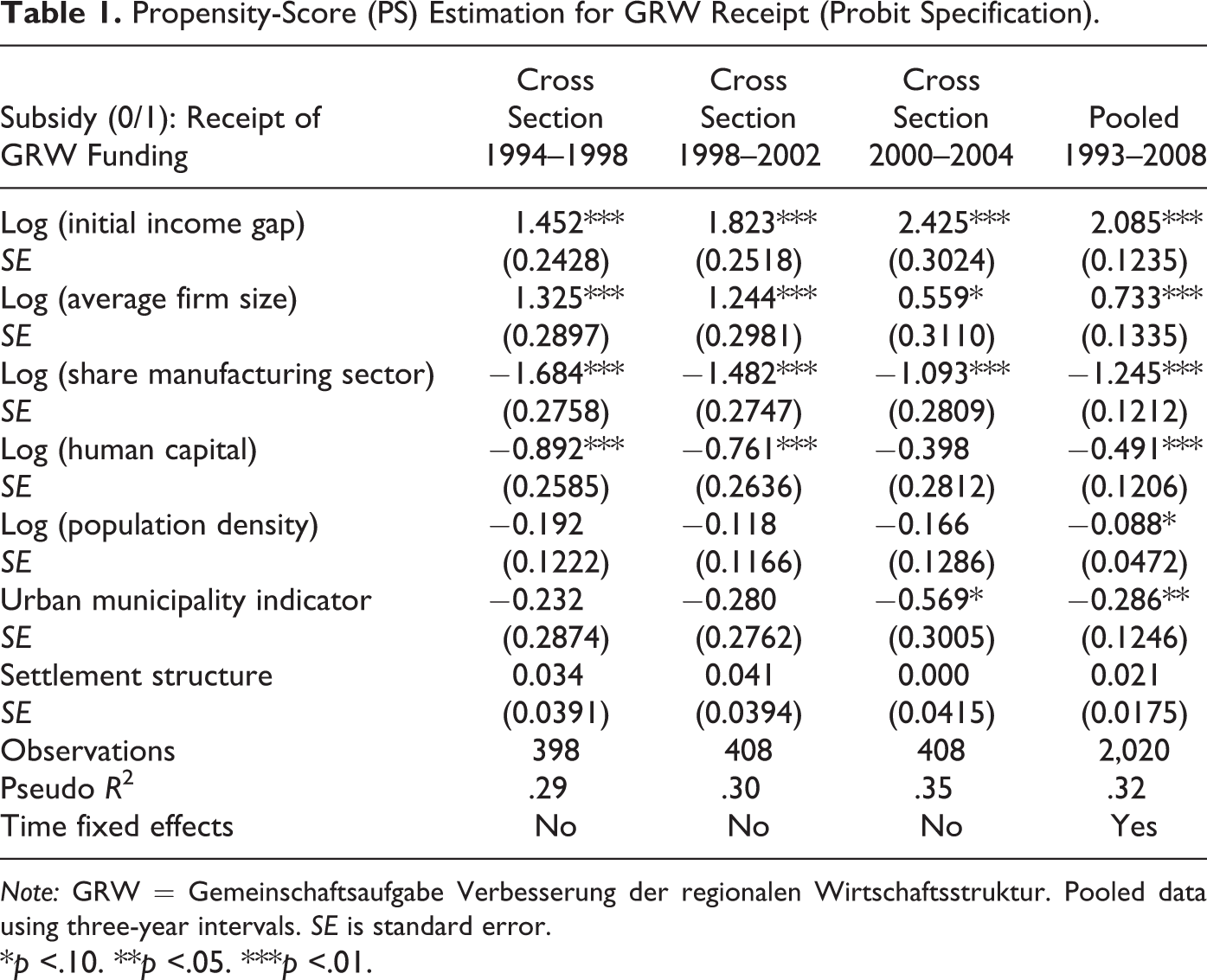
Note: GRW = Gemeinschaftsaufgabe Verbesserung der regionalen Wirtschaftsstruktur. Pooled data using three-year intervals. SE is standard error.

*p <.10. **p <.05. ***p <.01.

The remaining variables (population density, urban municipality indicator, and settlement structure) turn out to be statistically insignificant in most specifications. Only for the pooled specification do we get empirical evidence for a negative correlation of population density and the urban municipality indicator with the receipt of GRW funding, indicating that GRW funds—controlling for the city status—were mainly directed to agglomerated regions.

Having estimated the propensity score as the prerequisite for the selection of an appropriate comparison group, we can proceed with the actual matching. We chose the k nearest neighbor algorithm, where each treated region is matched by its five (k = 5) nearest neighbors (NN) measured in terms of the estimated propensity score according to Table 1. We further apply a common support restriction to our 5-NN matching routine in order to minimize the risk of bad matches and to avoid introducing bias. The results for the different sample designs are shown in Table 2. The table reports both the mean value of labor-productivity growth for the treated and the nontreated comparison group.

Table 2.

Nearest Neighbor (k = 5) Matching and Rosenbaum Bounds.

Outcome: Average Growth Rate of Labor Productivity	Cross Section 1999–2004	Cross Section 2003–2007	Cross Section 2005–2008	Pooled Three-year Lead
Mean of treated	0.019	0.023	0.024	0.023
Number (common support)	214 (191)	210 (189)	183 (132)	1,027 (858)
Mean of control	0.018	0.019	0.019	0.018
Number (common support)	184 (184)	198 (198)	225 (225)	993 (993)
τ_ATET	0.001	0.004**	0.006**	0.005***
SE	(0.0021)	(0.0019)	(0.0024)	(0.0016)
SB_before (in percentage)	51.0	49.9	54.6	52.3
SB_after (in percentage)	22.0	27.2	19.5	19.2
Ex post pseudo R ²	.087	.119	.086	.120
LR test	46.1***	62.2***	31.3***	283.2***
Γ₁	0.001	0.004***	0.005***	0.004***
p Value	(.15)	(.00)	(.00)	(.00)
Γ_1.5	−0.001	0.002**	0.003**	0.000
p Value	(.92)	(.05)	(.03)	(.31)
Γ₂	−0.003	0.000	0.001	−0.002
p Value	(.99)	(.49)	(.28)	(.99)

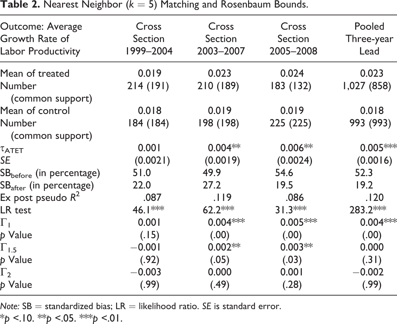
Note: SB = standardized bias; LR = likelihood ratio. SE is standard error.

*p <.10. **p <.05. ***p <.01.

As outlined above, for the different cross-sectional sample designs, we use an evaluation interval of five years, which is not allowed to overlap with the sample period for the propensity-score estimation in order to eliminate direct feedback effects. To illustrate this point, we estimate the outcome difference between treated and nontreated throughout the year 1999–2004 if the propensity score has been calculated for the period 1994–1998 and so forth. For the pooled data case, we use a three-year lead in the matching approach compared to the calculation of the associated propensity score. As the table shows, the estimated ATET parameter (τ_ATET) turns out to be positive and statistically significant for most time periods except for the first evaluation period 1999–2004. While the latter result may be motivated by a general business cycle downturn for that period, which also led to a significant reduction in the growth rate differential among German regions, the general impression from Table 2 is that growth in labor productivity is higher for GRW-funded regions compared to non-funded comparison units. The additional growth impulse is around 0.5 percentage points, which is about 20 percent of the total growth rate of treated regions.

To evaluate the sensitivity of the obtained results with regard to the “balancing properties” of propensity-score estimation, we compute the SB before and after estimation as proposed by Rosenbaum and Rubin (1983). As shown in Table 2, the SB based on the sample mean of subsidized and nonsubsidized regions is strongly reduced after matching (e.g., from 52 percent before matching to 19 percent after matching). However, as Caliendo and Kopeinig (2008) point, one problem associated with the SB criterion is that it does not provide a clear statistical indication for the success of the matching approach.

Another approach to evaluate the matching success is to use the pseudo R ² test proposed by Sianesi (2004). The approach involves a reestimation of the propensity score model only for the matched sample and then a comparison of the resulting pseudo R ² to the one obtained before matching. Since matching should balance the two groups, the pseudo R ² based on the matched sample should be low. As shown in Table 2 (compared to Table 1), the ex post pseudo R ² indeed drops by almost two-thirds of its initial “fit” (8–12 percent compared to 29–35 percent in the first-stage estimation). However, if we additionally compute a likelihood ratio test of whether the ex post pseudo R ² is statistically different from zero, the null hypothesis of zero explanatory power of the covariates in the matched sample is still rejected. This result raises some critical reflections on the reliability of the estimation results, given that a complete balancing of covariates is not possible for the sample at hand.

The implication of the likelihood ratio test is that the regional variation captured by the set of covariates may not be sufficient in order to isolate the causal effect of GRW on productivity growth. Stated differently, the assumption of conditional independence is less plausible in the present situation. Of course, the result is not surprising given the rather small set of regional entities at hand (N = 413), where only few covariates are at our disposal while the regional units itself form aggregated observations stemming from complex structural interdependencies at the subregional level. Nevertheless, as outlined in Reed and Rogers (2003), even under conditions of imperfect matching, the quasi-experimental control group estimator tends to be less biased compared to conventional regression, particularly if the relationship between the outcome variable of interest and the policies under study is nonlinear and policy adoption is nonrandom. The reduction in the SB as well as the pseudo R ² thus hint at the fact that the chosen matching approach—although not providing a perfect match—at least delivers a more appropriate weighting of subsidized and nonsubsidized comparison regions.

As a second sensitivity test, we apply the Rosenbaum bounding approach to quantify the probability that, for two regions with identical observed covariates, their chances of receiving GRW subsidy actually differ due to unobservable characteristics. If the latter probability is not zero, both regions will differ in their odds of receiving a subsidy by a factor that involves a parameter Γ. The computation of different values for Γ in Table 2 reveals that an unobserved factor needs to cause the odds ratio to differ by at least a factor of 1–1.5 in order to result in statistically insignificant outcome differences as a worst-case scenario. To illustrate the magnitude of a hidden bias that would force us to revise our statistical findings, we can equate the magnitude of this bias in terms of equivalent effects for observed covariates for which we can actually calculate it. For instance, a critical level of Γ = 1.5 is attained at a difference in human-capital endowments of more than 3.5 percent (with the sample mean being equal to 7 percent). Thus, the unobserved effect needs to be rather substantial compared to the distribution of the variable in order to have a statistically significant impact on the obtained result.

As a final robustness check, we also compare the estimated ATET parameter for alternative matching routines as well as a conventional ordinary least squares (OLS) approach. The results for the pooled specification (last column in Table 2) are shown in Table 3. As commonly applied in the microeconometric literature, next to the standard 5-NN matching routine, we thus also estimate the GRW policy impact on growth using radius, kernel, Mahalanobis distance, and stratification-based matching algorithms (for a description, see, for instance, Caliendo and Kopeinig 2008). As the table shows, the estimated τ_ATET is statistically significant for all applied matching algorithms and varies between 0.4 and 0.7 percentage points. These results thus closely resemble the estimation parameter in the 5-NN matching approach from above. The OLS estimates in the last column of Table 3 also turn out to be statistically significant (however, with a value of 0.2 percentage points, the estimated outcome difference is somewhat smaller compared to the matching results).

Table 3.

ATET Estimates for Alternative Matching Routines and OLS Regression.

	Stratification	Radius	Kernel	Mahalanobis	OLS
τ_ATET	0.007***	0.004***	0.005**	0.004***	0.002**
SE	(0.0010)	(0.0011)	(0.0021)	(0.0012)	(0.0010)

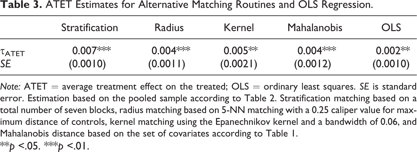
Note: ATET = average treatment effect on the treated; OLS = ordinary least squares. SE is standard error. Estimation based on the pooled sample according to Table 2. Stratification matching based on a total number of seven blocks, radius matching based on 5-NN matching with a 0.25 caliper value for maximum distance of controls, kernel matching using the Epanechnikov kernel and a bandwidth of 0.06, and Mahalanobis distance based on the set of covariates according to Table 1.

**p <.05. ***p <.01.

Keeping the potential pitfalls in mind, we may thus carefully argue that we have established a positive effect of GRW receipt on regional productivity growth. For the pooled specification, we thus obtain—on average—an additional annual growth effect for labor productivity of roughly 0.5 percentage points for GRW-funded regions. On top of this result, we finally want to take a closer look at the relationship between the actual funding volume and the regional productivity growth performance. This allows us to identify a maximum level of funding with positive marginal growth effects, that is, the level beyond no further growth effects can be observed. This second step involves the use of a GPS to compute dose–response functions.

In Table 4, we report the OLS estimates for the GPS estimates, where the dependent variable is the GRW intensity defined as GRW volume per unit of labor force (in 1,000€) for German NUTS 3 regions.¹⁴ In order to have a sufficiently high number of observations, we focus on two pooled specifications here:¹⁵ (1) a pooled model based on three-year averages for the period 1993–2008 in analogy to the binary matching approach outlined above and (2) a pooled model with annual observations. The set of regressors comprises lagged levels and growth rates of labor productivity and employment, as well as the investment intensity, the average firm size, foreign turnover, the share of manufacturing sector in total employment, human capital, population density, and the two indicator variables for the municipality status and settlement structure as introduced above.

Table 4.

Generalized Propensity-Score (GPS) Estimation.

Treatment: GRW Intensity	Three-year Interval 1993–2008	Annual 1993–2008
Log (lagged labor productivity level)	−0.159***	−0.127***
SE	(0.0197)	(0.0146)
Log (lagged labor productivity growth)	9.158***	9.425***
SE	(2.687)	(1.562)
Log (lagged employment level)	−0.078	0.049
SE	(0.1705)	(0.1261)
Log (lagged employment growth)	0.754	3.451
SE	(0.1891)	(3.2264)
Log (investment intensity)	0.755***	0.774***
SE	(0.1891)	(0.1255)
Log (average firm size)	−0.502	−0.811**
SE	(0.3463)	(0.2563)
Log (foreign turnover)	−0.135	−0.358***
SE	(0.1457)	(0.1036)
Log (share manufacturing sector)	0.219	0.514**
SE	(0.2679)	(0.2035)
Log (human capital)	3.133***	3.456***
SE	(0.3191)	(0.2281)
Log (population density)	−0.121	−0.095
SE	(0.1172)	(0.0641)
Net migration indicator	−1.056***	−0.786***
SE	(0.2178)	(0.1325)
Urban municipality indicator	0.209***	1.102***
SE	(0.0429)	(0.2231)
Settlement structure	0.067***	0.239***
SE	(0.0177)	(0.0319)
Observations	820	1,832
Time fixed effects	Yes	Yes
Kolmogorov–Smirnov test	0.032	0.014
p Value	(.36)	(.84)

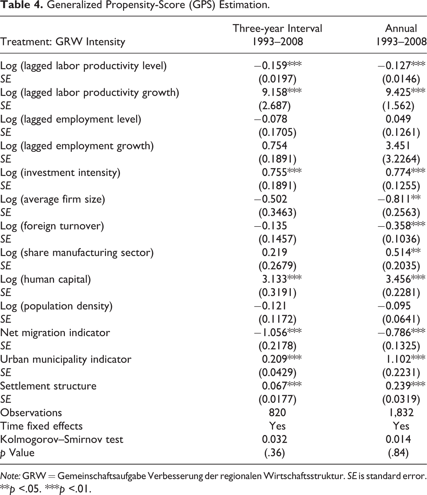
Note: GRW = Gemeinschaftsaufgabe Verbesserung der regionalen Wirtschaftsstruktur. SE is standard error.

**p <.05. ***p <.01.

Since the GPS approach requires normally distributed residuals, we chose a Box–Cox transformation for our dependent variable in Table 4. The latter transformation is the only operationalization that ensures normally distributed errors as indicated by the results of a Kolmogorov–Smirnov test conducted for the variable in levels, logarithmic, as well as Box–Cox transformation. Based on the estimated GPS as well as the treatment variable GRW, we can then compute the dose–response function by first regressing:¹⁶

E [y_{i} | G R W_{i}, G P S_{i}] = α_{0} + α_{1} G R W_{i} + α_{2} G R W_{i}^{2} + α_{3} G P S_{i} + α_{4} (G R W_{i} \times G P S_{i}),

and using the obtained parameters to estimate the average potential outcome at each subsidy level τ:

E [y_{i} | {\hat{G R W}}_{i}, G P S_{i}] = \frac{1}{N} \sum_{i = 1}^{N} [{\hat{α}}_{0} + {\hat{α}}_{1} τ + {\hat{α}}_{1} τ^{2} + {\hat{α}}_{3} G P S (τ, X_{i}) + {\hat{α}}_{4} (τ \times G P S (τ, X_{i}) τ] .

Additionally, the first derivative of the dose–response function with respect to the GRW transfer intensity can be computed as the so-called treatment effect function. As Becker et al. (2012) point out, the latter can be used to infer the maximum desirable subsidy level of regional policy. In order to reduce the sensitivity of the estimates with respect to large outliers, we restrict the calculation of the dose–response function up to the 90th percentile of the distribution of GRW funding.

The dose–response function shows how labor-productivity growth responds to changes in the GRW intensity. In order to interpret the results of the estimated dose–response function as shown in Table 5, we plot the dose–response and treatment effect functions in Figure 2. Of particular interest is the graph of the treatment effect function on the right-hand side of Figure 2, since it allows us to identify the subsidy level which is associated with a zero marginal increase in regional productivity growth. As the figure shows, this is the case for a subsidy level of approximately 8 (in its Box–Cox transformation), which corresponds to a GRW intensity of roughly €105,000 per unit of labor force and is about two-thirds of the maximum observed funding intensity (67th percentile of the distribution of GRW intensity).¹⁷

Figure 2.

Dose–response and treatment effect function for GRW intensity. GRW = Gemeinschaftsaufgabe Verbesserung der regionalen Wirtschaftsstruktur.

Table 5.

Estimated Dose Response Function.

Outcome: Growth Rate of Labor Productivity	Three-year Interval	Annual
Outcome: Growth Rate of Labor Productivity	1993–2008	1993–2008
GRW	−0.003***	−0.002
SE	(0.0007)	(0.0096)
GRW²	0.0002***	0.0001
SE	(0.00006)	(0.0007)
GPS	−0.053*	−0.071*
SE	(0.0302)	(0.0383)
GRW × GPS	0.015***	0.016***
SE	(0.0037)	(0.0048)
Observations	820	1,832
Balancing property (F-test)	Reject	Reject
p Value	(.00)	(.00)

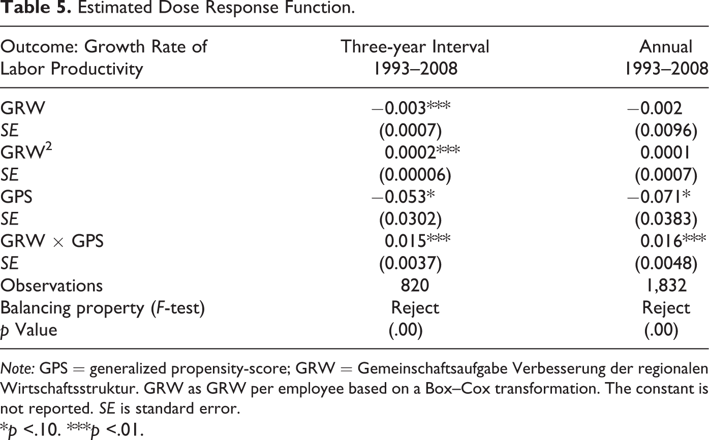
Note: GPS = generalized propensity-score; GRW = Gemeinschaftsaufgabe Verbesserung der regionalen Wirtschaftsstruktur. GRW as GRW per employee based on a Box–Cox transformation. The constant is not reported. SE is standard error.

*p <.10. ***p <.01.

For higher funding intensities, the GRW support is shown to be ineffective since it fails to induce an additional growth stimulus. Theoretically, a maximum desired subsidy level can be explained by the existence of diminishing returns to investment, that is, increasing funding intensities are associated with lower returns on investment. Additionally, we can observe that a minimum subsidy intensity is necessary to induce a positive growth stimulus (28th percentile of the distribution of GRW intensity, which corresponds to €16,000 per unit of labor force). Together with the maximum subsidy intensity, this results in an inverted U-shape of the treatment effect function as shown in Figure 2.

Our empirical results for the German GRW policy thus lie within the range of recent estimates at the EU level. While Becker et al. (2012), on one hand, find a rather high maximum subsidy intensity with only 18 percent of funded EU regions not reducing their growth performance in response of a reduction in funding, Mohl and Hagen (2008) do not get any evidence for a statistically significant and positive policy effect on EU regional growth, on the other hand. In comparison to recent analyses of the GRW with alternative empirical methods, our results mirror the positive effects typically reported in the literature (such as Alecke, Mitze, and Untiedt 2013; Röhl and von Speicher 2009; Schalk and Untiedt 2000). Although controlling for other factors such as spatial spillovers, these studies typically report an average effect of GRW funding on economic growth. If we replicate the latter approach and thus apply a linear regression model for the pooled annual model according to Table 4 augmented by the GRW intensity (in logarithmic transformation), we get an average growth effect of 0.0013 percent for a 1 percent increase in the GRW intensity. This average growth effect is consistent with the estimated range of effects as shown in the treatment effect function in Figure 2.

Our results have to be interpreted with some caution since the balancing property of the covariates in the matched sample is not fully satisfied (using an F-test as indicated in Table 5). This supports our expectations from above that, for regional data, where only a fixed (and small) set of covariates is available, it is rather hard to find perfect statistical twins resulting in an imperfect matching.

Does this then mean that one should not apply the matching approach in regional science and policy analysis at all? Clearly not, since this problem—as pointed out by Reed and Rogers (2003)—is not unique to the matching approach. To make this point clearer, one can simply bear in mind that the regression approach can be seen as a particular form of matching (for details, see Angrist and Pischke 2010). This close relationship between matching and regression may also be seen when one does a weighted regression, with the weights equal to the inverse probability of being selected into treatment. OLS may be viewed as matching with equal weights. The point is that the difficulty of comparing apples to apples and oranges to oranges in the matching context carries over to the regression framework. Moreover, given that the estimated dose–response function in Table 5 shows a clear nonlinear relationship between labor productivity growth and GRW funding, the simulation results in Reed and Rogers hint at the superiority of quasi-experimental control group approaches compared to conventional regression analysis for these settings.

Conclusion

In this article, we have applied quasi-experimental control group estimation to the analysis of regional policy in Germany. Starting with a short overview of recent advances in the field of control group analysis and microeconometric evaluation tools for the application in regional science and policy analysis, we have applied two complementary matching approaches for the evaluation of one Germany’s largest regional policy instruments, namely, the so-called “Gemeinschaftsaufgabe Verbesserung der regionalen Wirtschaftsstruktur” (GRW). The aim of the GRW is to foster regional growth in lagging regions through the provision of private sector investment grants as well as business-related infrastructure measures. Our results for the binary propensity-score matching approach show that GRW-funded regions indeed experienced a higher labor-productivity growth compared to non-funded regions throughout the sample period 1993–2008. This indicates that the GRW policy is successful in fostering convergence and equalizing standards of living in Germany. The result is robust to alternative matching routines as well as a linear benchmark regression model.

Using a GPS matching approach for the analysis of growth effects of the GRW intensity as a continuous subsidy-level variable, we also find that, up to a funding intensity of roughly two-thirds of the regional distribution of GRW payments, higher subsidies ensure higher productivity growth. Thus, in line with earlier work on German and EU regional funding, we obtain empirical evidence that regional policy is effective but only up to a certain subsidy level. The advantage of the GPS approach is that it allows us to identify a maximum treatment level as well as a minimum treatment subsidy intensity which is necessary to induce a positive growth stimulus, while conventional regression approaches, in comparison, are only able to estimate average growth effects of policy interventions. The use of quasi-experimental control group estimation can thus be seen as an important extension to standard policy analyses in regional science.

As our empirical application has also shown, there are some caveats, though. The most severe problem of the application of the experimentalist approach in regional science is that regional data exhibit special features that are likely to complicate empirical applications, particularly in terms of satisfying the so-called balancing property. As both the estimation results for the binary and for the GPS-based matching approaches have shown, it is very hard to find proper statistical twins for a fixed set of regional observations. However, as pointed out by Reed and Rogers (2003) in the conduct of Monte Carlo simulation exercises, even an imperfect matching approach typically results in a lower estimation bias compared to conventional regression estimators if policy adoption is nonrandom and the relationship between the outcome and policy variable is nonlinear. Both aspects apply for our sample setting. Another potential solution to circumvent the problem of imperfect matching could be to rely much more on individual- and firm-level data sets in the conduct of regional policy analysis. However, the disadvantage of such an approach is that it is typically not possible to identify regional net effects if the level of the analysis is the individual firm.

Moreover, the crucial assumption of “no general-equilibrium effects” (SUTVA) is difficult to justify in a regional setting, for instance, in the presence of spatial spillovers. Nevertheless, this does not mean that applications of the experimentalist school are a dead end in regional science and policy analysis. First, standard regression approaches have the same problems while lacking the transparency and rigor to isolate causal effects. Second, recent applications such as in Chagas et al. (2012) seek to find ways to include spatial effects in the analysis of matching models. An alternative approach would be to apply spatial filtering techniques in order to augment the (generalized) propensity-score matching approach. Thus, the quasi-experimental tools applied in this article—together with the broader field of experimental economics as outlined in Frank (2013)—appear to be an interesting addition to the standard toolkit in empirical regional science and policy analysis and mark a fruitful research agenda for the future.

Footnotes

Appendix

Table A1.

Descriptive Statistics of Variables in the Empirical Analysis.

Variable	Description	M	SD	Min.	Max.
Labor productivity	Regional GDP per employee (in 1,000€)	50.71	9.44	22.70	119.52
Employment	Employment level (in 1,000)	93.41	121.17	18.38	1,638.02
Investment intensity	Gross fixed capital formation in manufacturing sector as share of total turnover in manufacturing (in percentage)	4.92	4.02	0.46	76.50
Average firm size	Number of employees per firm	134.92	111.50	35.65	1,857.33
Foreign turnover	Share of foreign turnover in total turnover for manufacturing sector (in percentage)	29.25	14.46	0.00	420.31
Share manufacturing sector	Percentage share of employment in manufacturing sector relative to total employment	24.48	11.07	1.94	696.00
Human capital	Percentage share of school graduates with university qualification (in percentage)	7.14	3.36	1.93	25.27
Population density	Total population per square kilometer	14.33	94.93	0.38	2637.01
Net migration indicator	Binary indicator whether region has received a net surplus in migrants (internal and external), 0 otherwise	0.63	0.48	0	1
Urban municipality indicator	Binary indicator whether region belongs to a greater administrative district, 0 otherwise	0.73	0.44	0	1
Settlement structure	Indicators variable for different classes of settlement structure (classified according to an ordinal scale with 1 = highly agglomerated to 9 = highly peripheral)	5.39	2.52	1	9
GRW	Binary variable for receipt of GRW subsidies, 0 otherwise	0.45	0.50	0	1
GRW intensity	Volume of GRW subsidies per labor force (in 1,000€, T€), where labor force is defined as: $L F = \frac{1}{2} [(P o p_{t} - P o p_{t}^{< 18} - P o p_{t}^{> 65}) + (P o p_{t - 1} - P o p_{t - 1}^{< 18} - P o p_{t - 1}^{> 65})]$ , where Pop is population and the superscripts denote subgroups of population with less than eighteen years and more than sixty-five years, respectively. The subscript t and t–1 define the time periods	68.71	180.39	0.00	3,071.29

Note: GDP = gross domestic product; GRW = Gemeinschaftsaufgabe Verbesserung der regionalen Wirtschaftsstruktur. Descriptive statistics are given for the whole sample range of 1993–2008. Specific subsample information as used throughout the empirical applications can be obtained from the authors upon request.

Acknowledgments

The authors thank Torben Dall Schmidt and conference participants from the events listed in the Authors' Note for helpful suggestions. We also acknowledge the valuable comments of three anonymous reviewers and the editor, Sergio Rey.

Authors’ Note

Earlier versions of this article have been presented at the 50th ERSA Congress in Jönköping and the 51st ERSA Congress in Barcelona.

Declaration of Conflicting Interests

The author(s) declared no potential conflicts of interest with respect to the research, authorship, and/or publication of this article.

Funding

The author(s) received no financial support for the research, authorship, and/or publication of this article.

Notes

References

Alecke

Björn

Mitze

Timo

Untiedt

Gerhard

. 2013. “Growth Effects of Regional Policy in Germany: Results from a Spatially Augmented Multiplicative Interaction Model.” Annals of Regional Science 50:535–54.

Angrist

Joshua D.

Pischke

Jörn-Steffen

. 2010. “The Credibility Revolution in Empirical Economics: How Better Research Design is Taking the Con Out of Econometrics.” The Journal of Economic Perspectives 24:3–30.

Bartels

Cornelis P. A.

1982. “Measuring the effects of regional policy. An introduction.” Regional Science and Urban Economics 12(1):1.

Becker

Sascha O.

Caliendo

Marco

. 2007. “mhbounds—Sensitivity Analysis for Average Treatment Effects.” IZA Discussion Paper No. 2542, Institute for the Study of Labor, Bonn, Germany.

Becker

Sascha O.

Egger

Peter H.

Maximilian von Ehrlich

Maximilian

. 2010. “Going NUTS: The effect of EU Structural Funds on regional performance.” Journal of Public Economics 94(9-10):578–590.

Becker

Sascha O.

Egger

Peter H.

von Ehrlich

Maximilian

. 2012. “Too much of a good thing? On the growth effects of the EU’s regional policy.” European Economic Review 56(4):648–668.

Bia

Michela

Mattei

Alessandra

. 2008. “A Stata Package for the Estimation of the Dose–Response Function through Adjustment for the Generalized Propensity Score.” The Stata Journal 8:354–73.

Billings

Stephen

. 2009. “Do Enterprise Zones Work? An Analysis at the Borders.” Public Finance Review 37:68–93.

Bundesamt für Bauwesen und Raumordnung (BBSR). 2011. Laufende Raumbeobachtungen des Bundesinstitutes für Bau-, Stadt- und Raumforschung. Various issues. Bonn, Germany: Bundesamt für Bauwesen und Raumordnung.

10.

Caliendo

Marco

Kopeinig

Sabine

. 2008. “Some Practical Guidance for the Implementation of Propensity Score Matching.” Journal of Economic Surveys 22:31–72.

11.

Chagas

André Luis Squarize

Toneto

Rudinei

Azzoni

Carlos Roberto

. 2012. “A Spatial Propensity Score Matching Evaluation of the Social Impacts of Sugarcane Growing on Municipalities in Brazil.” International Regional Science Review 35:48–69.

12.

Deaton

Angus

. 2010. “Instruments, Randomization, and Learning about Development.” Journal of Economic Literature 48:424–55.

13.

Dehejia

Rajeev H.

Wahba

Sadek

. 1999. “Causal Effects in Nonexperimental Studies: Reevaluating the Evaluation of Training Programs.” Journal of the American Statistical Association 94:1053–62.

14.

Dehejia

Rajeev H.

Wahba

Sadek

. 2002. “Propensity Score-matching Methods Nonexperimental Causal Studies.” The Review of Economics and Statistics 84:151–61.

15.

Dell

Melissa

. 2010. “The Persistent Effects of Peru’s Mining Mita.” Econometrica 78:1863–903.

16.

DiPrete

Thomas

Gangl

Markus

. 2004. “Assessing Bias in the Estimation of Causal Effects: Rosenbaum Bounds on Matching Estimators and Instrumental Variables Estimation with Imperfect Instruments.” Sociological Methodology 34:271–310.

17.

Feser

Edward

. 2013. “Isserman’s Impact: Quasi-experimental Comparison Group Designs in Regional Research.” International Regional Science Review 36:44–68.

18.

Frank

Björn

. 2013. “Laboratory Evidence on Face-to-face: Why Experimental Economics is of Interest to Regional Economists.” International Regional Science Review. Published online June 13, 2012.

19.

Heckman

James J.

2010. “Building Bridges between Structural and Program Evaluation Approaches to Evaluating Policy.” Journal of Economic Literature 48:356–98.

20.

Heckman

James J.

Ichimura

Hidehiko

Todd

Petra

. 1997. “Matching as an Econometric Evaluation Estimator: Evidence from Evaluating a Job Training Program.” Review of Economic Studies 64:605–54.

21.

Heckman

James J.

Ichimura

Hidehiko

Todd

Petra

. 1998. “Matching as an Econometric Evaluation Estimator.” Review of Economic Studies 65:261–94.

22.

Heckman

James J.

Urzúa

Sergio

. 2010. “Comparing IV with Structural Models: What Simple IV can and Cannot Identify.” Journal of Econometrics 156:27–37.

23.

Hirano

Keisuke

Imbens

Guido W.

2004. “The Propensity Score with Continuous Treatments.” In Applied Bayesian Modeling and Causal Inference from Incomplete-Data Perspectives, edited by Gelman

Andrew

Meng

Xiao-Li

, 73–84. Chichester, UK: John Wiley.

24.

Holland

Paul W.

1986. “Statistics and Causal Inference.” Journal of the American Statistical Association 81:945–60.

25.

Holmes

Thomas J.

2010. “Structural, Experimentalist, and Descriptive Approaches to Empirical Work in Regional Economics.” Journal of Regional Science 50:5–22.

26.

Imbens

Guido W.

Wooldridge

Jeffrey M.

2009. “Recent Developments in the Econometrics of Program Evaluation.” Journal of Economic Literature 47:5–86.

27.

Isserman

Andrew M.

Merrifield

Scott

. 1982. “The use of control groups in evaluating regional economic policy.” Regional Science and Urban Economics 12(1):43–58.

28.

Leuven

Edwin

Sianesi

Barbara

. 2003. “PSMATCH2: Stata Module to Perform Full Mahalanobis and Propensity Score Matching, Common Support Graphing, and Covariate Imbalance Testing.” Statistical Software Components S432001, Boston College Department of Economics, Chestnut Hill, MA.

29.

Mohl

Philipp

Hagen

Tobias

. 2008. “Which is the Right Dose of EU Cohesion Policy for Economic Growth?” ZEW Discussion Paper No. 08-104, Zentrum für Europäische Wirtschaftsforschung, Mannheim, Germany.

30.

Moodie

Erica E. M.

Stephens

David A.

2007. “Estimation of Dose-Response Functions for Longitudinal Data using the Generalized Propensity Score.” Statistical Methods in Medical Research 21:149–66.

31.

Neyman

Jerzy

. 1923 [1990]. “On the Application of Probability Theory to Agricultural Experiments. Essays on Principles. Section 9.” Statistical Science 5:465–72.

32.

Reed

Robert W.

Rogers

Cynthia L.

2003. “A Study of Quasi-experimental Control Group Methods for Estimating Policy Impacts.” Regional Science and Urban Economics 33:3–25.

33.

Röhl

Klaus-Heiner

Speicher

Peggy P. von

. 2009. “Ostdeutschland 20 Jahre nach dem Mauerfall.” IW Positionen No. 41, Institut der deutschen Wirtschaft Köln, Cologne, Germany.

34.

Rosenbaum

Paul R.

2002. Observational Studies. 2nd ed. New York: Springer.

35.

Rosenbaum

Paul R.

Rubin

Donald B.

1983. “The Central Role of the Propensity Score in Observational Studies for Causal Effects.” Biometrika 70:41–55.

36.

Schalk

Hans Joachim

Untiedt

Gerhard

. 2000. “Regional Investment Incentives in Germany. Impacts on Factor Demand and Growth.” Annals of Regional Science 34:173–95.

37.

Sianesi

Barbara

. 2004. “An Evaluation of the Swedish System of Active Labor Market Programs in the 1990s.” The Review of Economics and Statistics 86:133–55.

38.

Stock

James H.

Trebbi

Francesco

. 2003. “Who Invented Instrumental Variable Regression?” The Journal of Economic Perspectives 17:177–94.

39.

Wooldridge

Jeffrey M.

2010. Econometric Analysis of Cross Section and Panel Data. 2nd ed. Cambridge, MA: MIT Press.