Regional Air Quality and Happiness in Germany

Abstract

Previous research has analyzed the impact of air pollution on life satisfaction (“happiness”) based on both subjective perceptions of environmental quality and objectively measured pollution data. This article combines these two types of environmental data in life satisfaction regressions and investigates using an instrumental variable (IV)-ordered probit approach whether perceived air quality is endogenous with respect to happiness. We find combining German 2004 socioeconomic panel data with annual readings for sulfur dioxide (SO₂), NO _x , and PM₁₀ by the Umweltbundesamt (UBA; German Environmental Protection Agency) for counties that people bothered by air pollution feel less happy but that simultaneously unhappy people feel more disturbed by air pollution. Controlling for this simultaneity in an IV-ordered probit approach reveals that perceived air pollution does not have a statistically significant effect on life satisfaction anymore. We also find econometric evidence that air pollution is fully capitalized in the housing market.

Keywords

discrete choice limited dependent variable models economic analysis methods other spatial analysis spatial analysis environment natural resources policy and applications other urban and regional issues urban and regional issues other human spatial structure human spatial structure spatial structure

Introduction

Life satisfaction approaches as a nonmarket valuation method for environmental quality have in recent years become increasingly more popular (van Praag and Baarsma 2005; Ferrer-i-Carbonell and Gowdy 2007; Levinson 2012; Luechinger 2009; MacKerron and Mourato 2009). Welsch (2002, 2006), Welsch and Kühling (2008), Ferreira and Moro (2010) and Frey, Leuchinger, and Stutzer (2010) give an overview of how to apply happiness research to environmental valuation. This popularity is related to the weaknesses of traditional economic valuation approaches. One of the traditional valuation approaches is the hedonic pricing approach, where the value of a public good is inferred from market transactions in private goods, in particular the housing market. The methodology is based on an equilibrium assumption in the housing market where rent compensates people for environmental disamenities (e.g., the costs of self-protection measures, higher risk premiums for insuring oneself against damages as well as for all noninsurable and nonavertable losses). In the market equilibrium, housing prices adjust to equalize utility across locations. Otherwise, some individuals would have an incentive to move from places with lower utility to places with higher utility.

If the equilibrium assumption holds and people are fully compensated, we would not find any environmental disamenities effects in life satisfaction regressions. However, the assumption of a spatial equilibrium in housing markets may be flawed, and, therefore, the benefits of a clean environment may be incompletely capitalized in housing markets. First of all, moving costs and other transaction costs may be high so that spatial equilibrium would not easily be achieved, which would lead to downward-biased coefficient estimates in hedonic housing price models. Second, government regulations in the housing market may constrain market compensation, either because housing prices are not allowed to adjust rapidly (e.g., as a result of rent control) or because there are constraints on the amount and variety of housing available (e.g., due to building regulations). Third, incomplete information or a distorted perception of the risk of pollution and its health effects may easily bias hedonic estimates. In particular, pollution levels and effects are not reflected in private markets if individuals are ignorant about their existence. Another traditional valuation approach, contingent valuation, directly asks people about their willingness to pay for environmental improvements or their willingness to accept payment in exchange for bearing a particular loss. Yet the approach is criticized among others, for not measuring revealed preferences, but asking hypothetical questions and for giving rise to problems of scope or embedding (Hausman 2012). The life satisfaction approach may be considered complementary to the hedonic pricing approach: it ideally measures the residual shadow costs for which people are not already compensated in the housing or labor markets and accounts for the additional disutility of environmental costs due to the nonexisting spatial equilibrium. It is often assumed that the combined willingness-to-pay figures derived from the regression coefficients, the one from the hedonic housing price model and the other one from the life satisfaction approach, represent a more accurate valuation of environmental (dis-)amenities. Yet Frey, Leuchinger, and Stutzer (2010) argue that under certain circumstances, the hedonic method and the life satisfaction approach can also measure similar phenomena and be considered substitutes.

We directly build on previous research that has suggested that some public goods or bads may not be entirely capitalized in market prices. However, if we follow the theory, then we could use the happiness regression approach also to test whether air pollution is fully capitalized in rent and the housing market is actually in spatial equilibrium with respect to the environmental quality variable of interest. To do so properly, it is imperative that the regression model is specified correctly. Luechinger (2009), for example, used an instrumental variable (IV) approach to account for the simultaneity of local sulfur dioxide (SO₂) improvements and regional economic conditions, both having an influence on well-being, however, with the opposite sign. Rehdanz and Maddison (2008) use reported subjectively perceived air pollution for their happiness regression, however, they fail to account for the endogeneity of this measure.

Inspired by the van Praag and Baarsma (2005) approach and further informed by MacKerron and Mourato (2009) and Ferreira and Moro (2010), the main contribution of this article is to extend their ideas to account for the endogeneity of a subjective perception of an externality and apply it to the happiness model by Rehdanz and Maddison (2008). Our primary interest is therefore the endogeneity between perceived air pollution and happiness. For that purpose, we use the IV-ordered probit approach developed by Rivers and Vuong (1988), which also allows explicit testing for endogeneity. Our rationale goes as follows: if air pollution affects life satisfaction above and beyond what is already capitalized in market rents (which can be analyzed using a hedonic housing price model), then ceteris paribus it should be the subjectively felt proportion of air pollution (perceived air quality) rather than the scientifically measured one. However, any subjective measure of air pollution could, in turn, be influenced by the person’s general happiness level. In other words, lower air quality may not only make people unhappy but also, simultaneously, unhappy people may feel more bothered by more air pollution.

Incomplete information and distorted risk perceptions can create the impression that people are strongly affected by air pollution, even if this is not reflected by measured pollution data. Yet Frey, Leuchinger, and Stutzer (2010) argue that the life satisfaction approach is less affected by distorted risk perceptions than the hedonic method because the welfare consequences of risk are primarily identified when the risk actually materializes. Moreover, the life satisfaction approach can capture the welfare consequences of health effects from air pollution even if individuals are ignorant about the causes, whereas incomplete information on health effects often leads to a downward bias in hedonic estimates (e.g., Smith and Huang 1995; Pope 2008).

A secondary interest of this study is, following the approach of Ferreira and Moro (2010), to identify whether or not air pollution is fully capitalized in rents, leading to the housing market being in spatial equilibrium with respect to air quality.

As in Rehdanz and Maddison (2008), we take life satisfaction data from the 2004 German socioeconomic panel (SOEP 2013), and as in Luechinger (2009), we take the air pollution measures from the 2004 Federal Environment Agency air quality monitoring data (UBA 2011). The article proceeds as follows. The second section provides a brief overview of related research. The third section elaborates on the methodology and the estimation strategy and describes the data. Results are presented in the fourth section. The fifth section concludes.

Previous Literature

A number of previous studies have explained differences in subjective well-being as a function of environmental (dis-)amenities and perceptions or attitudes. An international approach investigating NO _x emissions across many countries was followed in earlier research by Welsch (2002, 2006). Using aggregate, cross-sectional data for fifty-four countries, he found a negative effect of lower air quality on happiness. The main disadvantage of these studies is that, due to lack of data, life satisfaction and pollution levels are only assessed on the most aggregate level with no indication of within-country variability or real pollution exposure of individuals. Unobserved heterogeneity across individuals is therefore assumed to even out, and unobserved heterogeneity across countries needs to be controlled for. Moreover, country borders would hinder spatial equilibrium through migration.

Most of the more recent literature uses individual-level data and is restricted to one country or region. Luechinger (2009) uses individual-level panel data from the German SOEP and combines them with SO₂ data at the county level over a nineteen-year period (1985–2003).¹ To control for the simultaneity of local air quality and regional economic conditions, he uses exogenous environmental regulation, which mandates SO₂ emissions control equipment as an instrument. He finds that SO₂ emissions are capitalized in market rents only to a limited extent. In fact, Luechinger’s life satisfaction approach estimates a willingness-to-pay value for SO₂ reduction of five to fifty times higher than compatible hedonic housing price models.

Using SOEP data for 2004, Rehdanz and Maddison (2008) incorporate into a model estimating life satisfaction subjective measures of local environmental quality, including air pollution. Their results again support the idea that air pollution is not entirely capitalized in market rents. However, this study has one main shortcoming: the endogeneity of subjective air pollution measures is not accounted for.

Both Luechinger (2009) and Rehdanz and Maddison (2008) present some evidence that there may be a degree of spatial disequilibrium with respect to air quality in Germany. Levinson (2012) undertook a study comparable to Luechinger’s (2009) for the United States. Using the General Social Survey data, he found significantly negative effects on happiness only for PM₁₀, but not for ozone, SO₂, or carbon monoxide (CO). These results could indicate that in the United States, there is spatial equilibrium for some pollutants. However, Levinson (2012) suggests that his study covers many areas without significant ozone and SO₂ problems so that significantly negative impacts on happiness would not be measured correctly.

A weakness of the above-mentioned studies is the high spatial aggregation of the environmental quality variables, such as it is the case for, that is, county-level data. This issue is addressed by MacKerron and Mourato (2009) who analyze willingness to pay for air quality in London, UK, focusing on NO _x . They collect original survey data for 400 Londoners and match them with pollutant concentrations in the immediate vicinity of their homes. Two happiness models are used, one with a subjective air quality measure as an independent variable and another one with scientific measurements of air quality. Both regressions indicate a statistically significant and negative impact of air pollution on life satisfaction. The authors even discussed the possibility that the subjective air quality measure variable is endogenous; however, they did not push the argument further and just compared both the subjective and scientific measurement coefficients but did not address the issue econometrically.

In the case of Ireland, Ferreira and Moro (2010) find that PM₁₀ reduces subjective well-being. Furthermore, they discuss the limitation of environmental valuation based on just hedonic models in the presence of spatial disequilibrium, a discussion that was initiated by van Praag and Baarsma (2005). This important study addresses airport noise in Amsterdam, the Netherlands, to supplement hedonic housing price valuation results for a cost–benefit analysis. They assume spatial disequilibrium in housing market from the onset, and, unlike other authors, explicitly discuss the problem from the theoretical point of view in order to develop empirical solutions. They first regress an objective indicator of noise on life satisfaction (using measured noise levels, the frequency of flights, and a correcting factor for day and night traffic) but do not find a significantly negative influence. Similar to MacKerron and Mourato (2009), they use disaggregated noise data at the postcode level, which is reasonable given the highly localized influence of noise. Second, they replace the objective noise indicator by an ordinal indicator of subjective noise nuisance that is corrected for individual characteristics (like housing attributes, family size, and presence at home during the day). In this specification, the noise variable has a significantly negative impact on well-being. Van Praag and Barsma (2005) also compute the residual shadow costs for changes in the noise level that are not compensated in the housing market. In contrast to Rehdanz and Maddison (2008), they model subjective noise perception explicitly to include the fitted values into the final happiness regression. Yet they still fail to explicitly account for the endogeneity issue in the econometric model.

Ferrer-i-Carbonell and Gowdy (2007) study the relationship between individual environmental attitudes and subjective measures of well-being, an issue that is not treated explicitly in the above-mentioned literature using perception data. The former are conceptualized on the basis of subjective ratings and questions regarding concerns about ozone destruction and species extinction. According to their baseline regression, they find a negative coefficient for concern about ozone destruction on individual’s well-being and a positive one for concern about species extinction. They notice that environmental attitudes may correlate with excluded explanatory variables or unobserved individual personal traits that influence happiness. Ferrer-i-Carbonell and Gowdy add dummy variables to capture the natural environment where individuals live. They find that the negative effect of being concerned about the ozone layer and the positive effect of caring about animal extinction on happiness in their baseline regression still holds. To account for psychological traits, a set of ten individually self-reported mental health characteristics are included (e.g., feeling of strain, worrying a lot, etc.). Again, no major changes are observed for the environmental attitude variables. While they addressed the omitted variable problem, they fell short of identifying and explicitly modeling the endogeneity of personal traits with respect to happiness.

Endogeneity in life satisfaction approaches have been discussed from early on, mainly with respect to the income variable (Frey and Stutzer 2002). The basic argument is that not only higher income makes a person happier but also simultaneously reversed causation holds as well, and happier people are also more likely to have higher incomes. In fact, both Luechinger (2009) and Levinson (2012) do account for the endogeneity of income in their respective analyses. However, the endogeneity of subjective air pollution measures is so far not econometrically addressed in happiness research. This is the starting point of our study.

Data and Model

The principal source of data in this study is the SOEP, which is a representative, longitudinal annual survey of socioeconomic characteristics for individuals and households in Germany that was started in 1984. Repeating waves of the survey focus on different topics, such as life satisfaction and perceived air pollution. Geocoded data can be used via remote access at the level of the 439 German counties.²

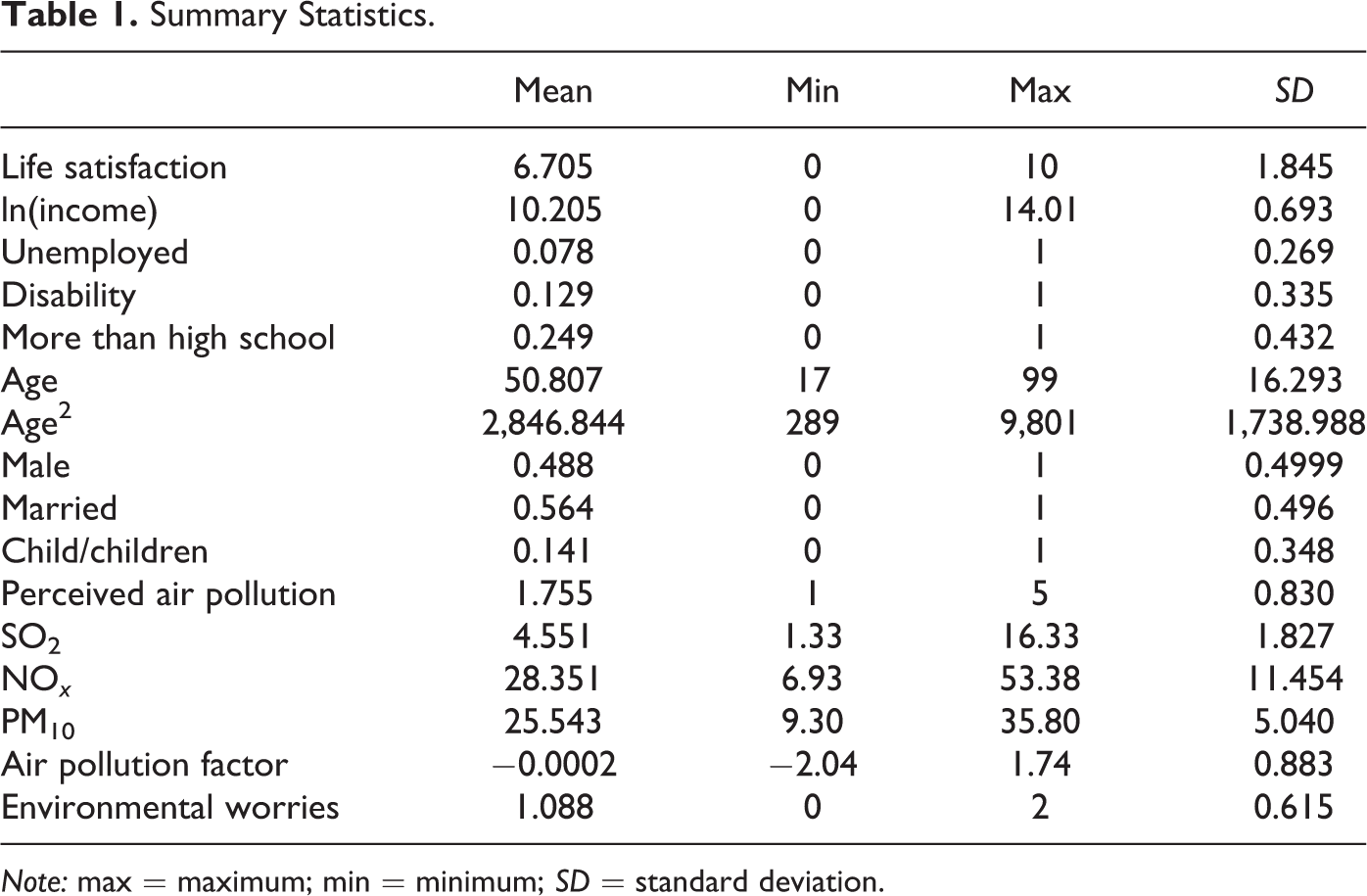
For our happiness model, we use 2004 personal data of the household heads, such as life satisfaction, income, employment status (unemployed), education (more than high school), age, gender (male), marital status, the existence of at least one child in the same household, and perceived air pollution (SOEP 2013). As the question on perceived air pollution is only asked every five years, 2009 is the only other year with available data. However, the year 2009 is marked by the economic crisis distorting the potential impact of perceived air pollution on happiness relative to 2004. Life satisfaction is ranked on an 11-point scale describing the degree of happiness. Perceived air pollution is surveyed on a 5-point scale. Table 1 exhibits the summary statistics of the final data set with all the included model variables.

Table 1.

Summary Statistics.

	Mean	Min	Max	SD
Life satisfaction	6.705	0	10	1.845
ln(income)	10.205	0	14.01	0.693
Unemployed	0.078	0	1	0.269
Disability	0.129	0	1	0.335
More than high school	0.249	0	1	0.432
Age	50.807	17	99	16.293
Age²	2,846.844	289	9,801	1,738.988
Male	0.488	0	1	0.4999
Married	0.564	0	1	0.496
Child/children	0.141	0	1	0.348
Perceived air pollution	1.755	1	5	0.830
SO₂	4.551	1.33	16.33	1.827
NO _x	28.351	6.93	53.38	11.454
PM₁₀	25.543	9.30	35.80	5.040
Air pollution factor	−0.0002	−2.04	1.74	0.883
Environmental worries	1.088	0	2	0.615

Note: max = maximum; min = minimum; SD = standard deviation.

The average life satisfaction score is about 6.7 and therefore in the upper half of the 11-point scale. The mean of ln(income) is about 10.2, which corresponds to about 27,000 Euros, and 7.8 percent are unemployed. These income and employment figures coincide closely with official statistics. About one-quarter of the participants have more education than high school. The mean age is about fifty-one years old. A little less than half of the people are male, while a little more than half are married. About 14 percent of the people have at least one child in their household. The average environmental worry score is around 1.1, pretty much in the center of the 3-point scale.

We estimate an ordered probit model to estimate a person’s level of life satisfaction. To account for endogeneity in the analysis, we apply a two-stage conditional maximum likelihood (2SCML) estimation method, developed by Rivers and Vuong (1988). The method calls for a first-step ordinary least squares (OLS) regression with the endogenous effect as the dependent variable on the IVs. The residuals of the first step together with the measured endogenous effect are then used in the second-step probit model (Wooldridge 2002). The model system looks as follows:

S t e p 1 : y_{1 i} = X_{i}' α_{1} + Z_{i}' α_{2} + ν_{i},

S t e p 2 : y_{2 i}^{*} = X_{i}' β_{1} + y_{1 i}' γ + u_{i},

w i t h y_{2 i}^{*} = \{\begin{matrix} 0 i f y_{2 i} \leq 0 \\ 1 i f 0 < y_{2 i} \leq μ_{1} \\ 2 {i f μ}_{1} < y_{2 i} \leq μ_{2} \\ . \\ . \\ . \\ 10 i f μ_{9} < y_{2 i} \end{matrix},

where y _1i is the hypothesized endogenous effect (air pollution perceived by individual i); y _2i * is the ordered happiness score for individual i; y _2i is the latent happiness level for individual i; μ _j is the happiness level threshold values for 1 ≤ j ≤ 9; X_i represents a vector of observed personal characteristics; Z_i represents a vector of observed instruments (measured air quality); α, β, and γ are regression coefficients; and ν _i and u_i are unobserved error terms.

We assume (ν _i , u_i ) are independent and identically distributed, with a mean of zero. The parameters in equation (2) are not identified without a further normalization. Following Wooldridge (2002), we choose var(u) ≡ 1 and set u_i ≡ ν _i ′λ + η _i with λ = cov(ν, u)/var(ν). Under these assumptions, we can now rewrite equation (2) as:

y_{2 i}^{*} = β_{0} + X_{i}' β_{1} + y_{1 i}' γ + ν_{i}' λ + η_{i} .

Rivers and Vuong’s 2SCML estimation method proceeds as follows: Since u_i is not observed, we first estimate this by running the OLS regression in equation (1) of the hypothesized endogenous variable y_1i on the observed variables X_i , Z_i , and saving the least square residuals. Then in the second step, we run the probit model of y _2i * with X_i , y _1i and the least square residuals from the first step as explanatory variables. We obtain consistent estimators of the scaled coefficients, which is sufficient for our purpose since we are only interested in the significance and the sign of the coefficients. A convenient feature of the 2SCML procedure is that the estimate of λ can be directly used to test for exogeneity. The probit z-statistic on the least square residuals from the first step is a valid test of the null hypothesis that y _1i is exogenous (H₀: λ = 0).

We include a total of two instruments. As the first instrument, we use county-based air quality readings of 2003 to 2005 annual mean concentration for SO₂, NO _x , and PM₁₀ collected by the monitoring network of the 16 state environmental agencies and provided by the Federal Environmental Agency of Germany for the years 2000 to 2009 (UBA 2011). In total, there are 475 SO₂ monitoring stations, 652 NO _x monitoring stations, and 688 PM₁₀ monitoring stations, which are all geocoded and attributed to their respective counties. To match pollution data and survey data, we use the mean value of concentrations per county (in case there is more than one monitor per county, which is true in about 20–25 percent of all the counties with monitors). In all, 34–40 percent of the 439 German counties do not have any monitor (149 for NO _x , 177 for SO₂, and 153 for PM₁₀). However, these were all rural counties and thus had only a few SOEP participants who were typically not exposed to a lot of air pollution.³ This process reduced the original SOEP data set only by about 10 percent from 8,810 to 7,874 observations.

Since the three air quality variables are highly correlated with each other, mainly because of them being coproduced, we summarize the information from all pollution measures into one variable using factor analysis. This has the added benefit of minimizing the danger of overidentification. In Table 2, it can be seen that the air pollution factor is more correlated with the endogenous variable than each of the three components.

Table 2.

Correlation Table.

	Perceived air pollution	SO₂	NO _x	PM₁₀	Air pollution factor	Environmental worries
SO₂	0.0729
NO _x	0.1460	0.3594
PM₁₀	0.1257	0.2635	0.7631
Air pollution factor	0.1476	0.4252	0.9529	0.9135
Environmental worries	0.1133	0.0317	0.0130	0.0130	0.0243
Life satisfaction	−0.1105	0.0512	0.0678	0.0203	0.0532	−0.0379

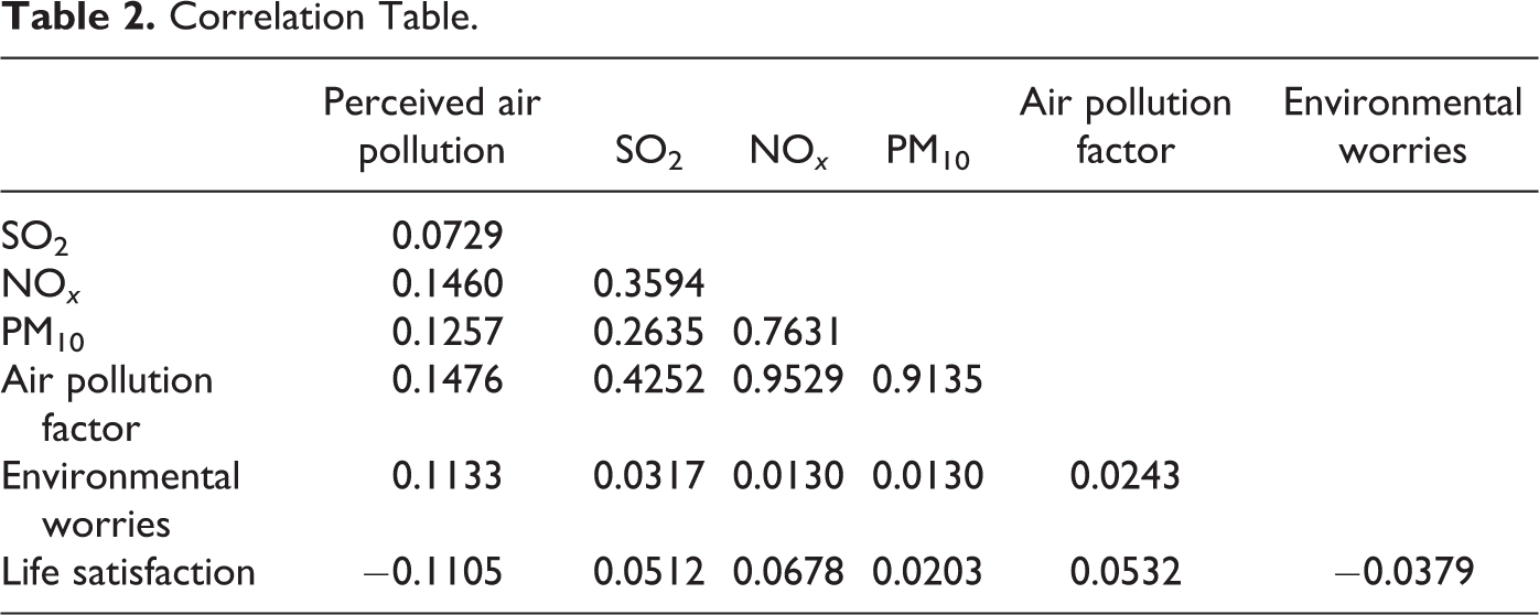
As the second instrument, we take the subjectively stated variable, environmental worries, which is reported on a 3-point scale. Table 2, which reports the correlations between the depend variable, the instruments, and the endogenous variable, shows that both the air pollution factor and the environmental worries are correlated with the endogenous variable, perceived air pollution, but not with each other, which makes both instruments complementary. Furthermore, neither of the two instruments is correlated with the dependent variable, life satisfaction, which makes them both good instruments.

Results and Discussion

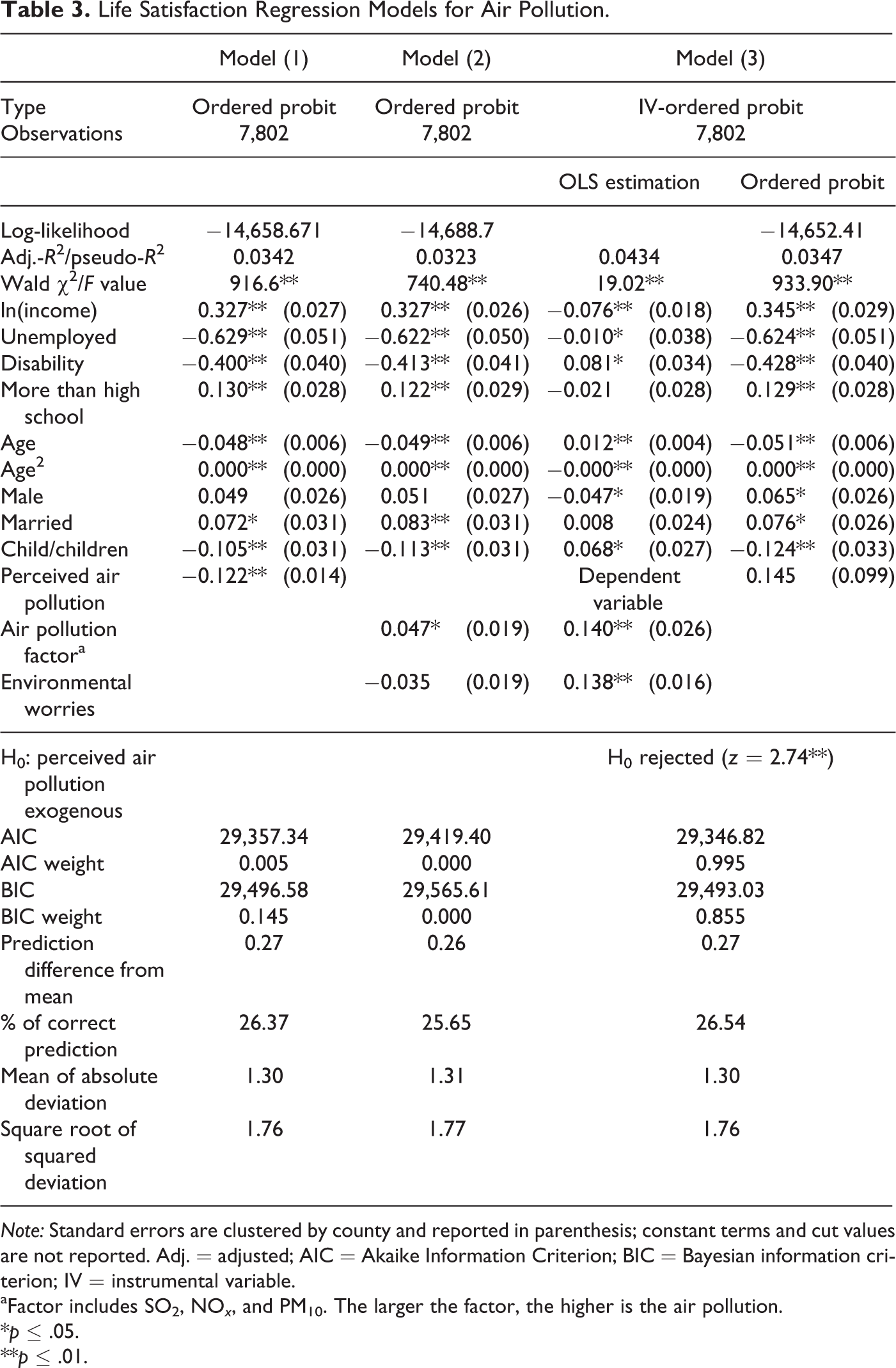
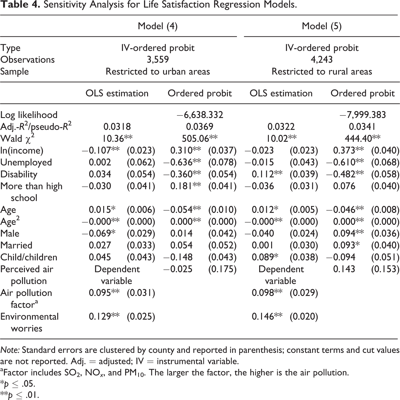
We ran a total of five models: The first two models were straightforward-ordered probit models assuming no endogeneity. Model (1) uses just the perceived air pollution variable; Model (2) replaces the perceived air pollution variable with the factor of SO₂, NO _x , and PM₁₀. Model (3), the main model, is the IV-ordered probit model that accounts for the endogeneity of perceived air pollution by using the air pollution factor together with the environmental worries measurement as instruments. Models (4) and (5) are estimated for a sensitivity analysis, where the data set was split into urban and rural observations to check for systematic differences. The regression results for all models are displayed in Tables 3 and 4, with all error terms being clustered by the Kreise/county.

Table 3.

Life Satisfaction Regression Models for Air Pollution.

	Model (1)		Model (2)		Model (3)
Type	Ordered probit		Ordered probit		IV-ordered probit
Observations	7,802		7,802		7,802
					OLS estimation		Ordered probit
Log-likelihood	−14,658.671		−14,688.7				−14,652.41
Adj.-R ²/pseudo-R ²	0.0342		0.0323		0.0434		0.0347
Wald χ²/F value	916.6**		740.48**		19.02**		933.90**
ln(income)	0.327**	(0.027)	0.327**	(0.026)	−0.076**	(0.018)	0.345**	(0.029)
Unemployed	−0.629**	(0.051)	−0.622**	(0.050)	−0.010*	(0.038)	−0.624**	(0.051)
Disability	−0.400**	(0.040)	−0.413**	(0.041)	0.081*	(0.034)	−0.428**	(0.040)
More than high school	0.130**	(0.028)	0.122**	(0.029)	−0.021	(0.028)	0.129**	(0.028)
Age	−0.048**	(0.006)	−0.049**	(0.006)	0.012**	(0.004)	−0.051**	(0.006)
Age²	0.000**	(0.000)	0.000**	(0.000)	−0.000**	(0.000)	0.000**	(0.000)
Male	0.049	(0.026)	0.051	(0.027)	−0.047*	(0.019)	0.065*	(0.026)
Married	0.072*	(0.031)	0.083**	(0.031)	0.008	(0.024)	0.076*	(0.026)
Child/children	−0.105**	(0.031)	−0.113**	(0.031)	0.068*	(0.027)	−0.124**	(0.033)
Perceived air pollution	−0.122**	(0.014)			Dependent variable		0.145	(0.099)
Air pollution factor^a			0.047*	(0.019)	0.140**	(0.026)
Environmental worries			−0.035	(0.019)	0.138**	(0.016)
H₀: perceived air pollution exogenous					H₀ rejected (z = 2.74**)
AIC	29,357.34		29,419.40		29,346.82
AIC weight	0.005		0.000		0.995
BIC	29,496.58		29,565.61		29,493.03
BIC weight	0.145		0.000		0.855
Prediction difference from mean	0.27		0.26		0.27
% of correct prediction	26.37		25.65		26.54
Mean of absolute deviation	1.30		1.31		1.30
Square root of squared deviation	1.76		1.77		1.76

Note: Standard errors are clustered by county and reported in parenthesis; constant terms and cut values are not reported. Adj. = adjusted; AIC = Akaike Information Criterion; BIC = Bayesian information criterion; IV = instrumental variable.

^aFactor includes SO₂, NO _x , and PM₁₀. The larger the factor, the higher is the air pollution.

*p ≤ .05.

**p ≤ .01.

Table 4.

Sensitivity Analysis for Life Satisfaction Regression Models.

	Model (4)				Model (5)
Type	IV-ordered probit				IV-ordered probit
Observations	3,559				4,243
Sample	Restricted to urban areas				Restricted to rural areas
	OLS estimation		Ordered probit		OLS estimation		Ordered probit
Log likelihood			−6,638.332				−7,999.383
Adj.-R ²/pseudo-R ²	0.0318		0.0369		0.0322		0.0341
Wald χ²	10.36**		505.06**		10.02**		444.40**
ln(income)	−0.107**	(0.023)	0.310**	(0.037)	−0.023	(0.023)	0.373**	(0.040)
Unemployed	0.002	(0.062)	−0.636**	(0.078)	−0.015	(0.043)	−0.610**	(0.068)
Disability	0.034	(0.054)	−0.360**	(0.054)	0.112**	(0.039)	−0.482**	(0.058)
More than high school	−0.030	(0.041)	0.181**	(0.041)	−0.036	(0.031)	0.076	(0.040)
Age	0.015*	(0.006)	−0.054**	(0.010)	0.012*	(0.005)	−0.046**	(0.008)
Age²	−0.000**	(0.000)	0.000**	(0.000)	−0.000**	(0.000)	0.000**	(0.000)
Male	−0.069*	(0.029)	0.014	(0.042)	−0.040	(0.024)	0.094**	(0.036)
Married	0.027	(0.033)	0.054	(0.052)	0.001	(0.030)	0.093*	(0.040)
Child/children	0.045	(0.043)	−0.148	(0.043)	0.089*	(0.038)	−0.094	(0.051)
Perceived air pollution	Dependent variable		−0.025	(0.175)	Dependent variable		0.143	(0.153)
Air pollution factor^a	0.095**	(0.031)			0.098**	(0.029)
Environmental worries	0.129**	(0.025)			0.146**	(0.020)

Note: Standard errors are clustered by county and reported in parenthesis; constant terms and cut values are not reported. Adj. = adjusted; IV = instrumental variable.

^aFactor includes SO₂, NO _x , and PM₁₀. The larger the factor, the higher is the air pollution.

*p ≤ .05.

**p ≤ .01.

Model (1) is similar to the one of Rehdanz and Maddison (2008), with perceived air pollution as an exogenous variable. All regression coefficients for the personal characteristics have the expected signs, documented in previous literature, and all but one (male) are also statistically significant at the 1 percent level: income increases happiness at a diminishing rate, unemployment depresses it, as does a disability, and more education than high school improves life satisfaction. People are the most happy when they are young and again when they are older, but life satisfaction is the lowest during the mid-life period. Men are happier than women. Although married people have a higher life satisfaction, the existence of at least one child in the household makes a person less happy. Finally, perceived air pollution decreases life satisfaction, just as it was reported in Rehdanz and Maddison (2008).

If perceived air pollution is replaced by the actual measurements of annual mean concentration for SO₂, NO _x , and PM₁₀ and environmental worries, as it is done in Model (2), we find that none of the regression coefficients for the personal variables change their sign or magnitude nor do they change their significance level. However, the air pollution factor becomes positive and significant at the 5 percent level, whereas the environmental worries coefficient is not significant at all. The contradicting results in Models (1) and (2) indicate the strong possibility of the perceived air pollution variable being endogenous, which we will test in Model (3).

Model (3) is the IV-ordered probit model, which consists of two different regressions. The first regression is an OLS estimation of perceived air pollution, displayed in the left column. Both instruments, the air pollution factor and the environmental worries measurement, have the expected positive sign and are significant at the 1 percent level. This means that people living in areas with lower air quality and/or with more environmental worries do in fact feel more bothered by air pollution. Although there is no formal test for weak instruments for instrumental probit models with clustered errors, a first approximation would be Staiger and Stock (1997), who claim that for a model with one endogenous variable, an F value higher than 10, which is definitely the case for Model (3) (F value 19.02), would ensure instruments to be not weak.

The second regression of the IV-ordered probit model, which is the ordered probit estimation, and reported in the right column, shows that perceived air pollution is no longer statistically significant, while all the other regression coefficients neither change their signs, magnitude, nor their significance level. In addition, the sign of the perceived air pollution variable is now positive, just as for the air pollution factor in Model (2). The test of the null hypothesis that perceived air pollution is exogenous is rejected at the 1 percent significance level. Both the lack of significance for the instrumented perceived air pollution regression coefficients and the result of the endogeneity test are strong evidence that the variable is indeed endogenous.

In addition, we use several diagnostic tools to determine whether Model (3) is superior to the previous two models. It turns out that Model (3) outperforms both models along most measures: The (more liberal) Akaike Information Criterion weight and the (stricter) Bayesian information criterion weight are by far the highest, both indicating clearly that Model (3) (with a probability of 99.5 percent and 85.5 percent, respectively) is comparatively the best specification (Wagenmakers and Farrell 2004). Although the prediction difference from the mean is lower in Model (2), Model (3) has more correct predictions than the other two models. In addition, the mean of the absolute deviation and the square root of the squared deviation, which weights higher deviations more, are both lower for Model (3) compared to Model (2), and are the same as Model (1).

Taking everything together, it can be said that Model (3) is the strongest one, which is further evidence in support of causality between happiness and perceived air pollution running both ways. This means that once simultaneity is controlled for, perceived air pollution does not have any statistically significant impact on life satisfaction anymore.

The results of Models (4) and (5) confirm the findings of Model (3). There are only a few marginal changes in the regression coefficients and none of significance for the instrumented perceived air pollution. Therefore, we have shown that model (1) can be improved upon by accounting for the endogeneity of the perceived air pollution measure. Also, we have shown for Model (2) that using the perceived air pollution measure as an instrumented endogenous variable corrects for the counterintuitive sign of the air quality factor coefficient.

As a secondary finding, our results exhibit some evidence that subjective air quality is capitalized in rents and a spatial equilibrium exists in the housing market with respect to air quality. With this analysis, we follow the approach by Ferreira and Moro (2010), which does not require any data on housing characteristics. The basic idea is the following: a utility-maximizing agent faces the trade-off of any characteristics in question, such as air pollution, which households are willing to pay for through housing location, and all other goods and services, based on the their tastes and preferences, their income, and relative prices. Although tastes and preferences are fixed and relative prices are determined in markets, only income should matter for happiness (which would be represented as the level of the indifference curve). This means in our case, that as long perceived air pollution is not significant, happiness cannot be improved by moving to another location, which can only happen if air pollution is fully capitalized in rents with the result of spatial equilibrium, but only for the one characteristic, air quality. Of course, our results neither state that air pollution does not reduce utility nor the possibility of spatial disequilibrium along another housing characteristic. Rather it just claims that the disutility stemming from air pollution, and only that characteristic, is fully compensated by lower housing cost. Therefore, the willingness to pay for reduced air pollution can only be identified through a hedonic housing price regression and not through a happiness model.

Conclusion

Based on a life satisfaction approach with German SOEP data and air quality measurements, we could show using an IV probit model that (1) the subjective variable “perceived air pollution” is endogenous and (2) air pollution is capitalized in market rents, indicating spatial equilibrium with respect to air quality. Our result is somewhat different to what Luechinger (2009) finds; Luechinger presented evidence of spatial disequilibrium for SO₂ emissions. However, he used data over a longer time period (1985–2003) during which new emissions regulation was introduced and air pollution decreased significantly. This change in air quality due to the new regulation would explain the interim spatial disequilibrium. Our findings, on the other hand, point to the fact that in the meantime, the housing market has adjusted and spatial equilibrium has been reached again. Our study also extends Rehdanz and Maddison (2008) who ignored the endogeneity of the same subjective air quality measure we use.

There are some limitations to our research: we did not have air pollution measurements for all counties causing the loss of about 10 percent of our observations. We considered generating the missing values with the help of a regression model but did not pursue this avenue for three reasons: first, modeled values are never as good as measured ones. Second, the benefit of adding 10 percent of the observations did not justify the cost of generating air quality values. And, third, all the missing measurements occur in rural areas, where there is generally much less of an air pollution issue. In fact, the regression results do not change at all if we just replace missing emission figures with the ones from the closest neighboring county.

The next limitation is that we assume linearity of the ordinal variable perceived air pollution in the first step of the IV estimation (OLS regression). In further robustness checks, which we did not report, we also ran the model with the ordinal variable perceived air pollution converted into a binary one but did not find any significantly different results.

Finally, the regression coefficients seem also robust, when each of the measured emissions (SO₂, NO _x , and PM₁₀) are included separately, as well as with different conversion definitions of the ordinal scales of the perceived air pollution variable (not reported, as well). Therefore, we are confident about the validity of our findings.

Footnotes

Acknowledgments

This article benefited greatly from comments by two anonymous referees. We also thank the German Institute for Economic Research (DIW) for providing us with the remote access to the SOEP data set.

Authors’ Note

All errors or omissions remain our responsibility.

Declaration of Conflicting Interests

The author(s) declared no potential conflicts of interest with respect to the research, authorship, and/or publication of this article.

Funding

The author(s) received no financial support for the research, authorship, and/or publication of this article.

Notes

References

Ferreira

Susanna

Moro

Mirko

. 2010. “On the Use of Subjective Well-being Data for Environmental Valuation.” Environmental and Resource Economics 46:249–73.

Ferrer-i-Carbonell

Ada

Gowdy

John M.

2007. “Environmental Degradation and Happiness.” Ecological Economics 60:509–16.

Frey

Bruno

Leuchinger

Simon

Stutzer

Alois

. 2010. “The Life Satisfaction Approach to Environmental Valuation.” Annual Review of Resource Economics 2:139–60.

Frey

Bruno S.

Stutzer

Alois

. 2002. “What Can Economists Learn from Happiness Research?” Journal of Economic Literature 40:402–35.

Hausman

Jerry

. 2012. “Contingent Valuation: From Dubious to Hopeless.” Journal of Economic Perspectives 26:43–56.

Levinson

Arik

. 2012. “Valuing Public Goods Using Happiness Data: The Case of Air Quality.” Journal of Public Economics 96:869–80.

Luechinger

Simon

. 2009. “Air Quality Using the Life Satisfaction Approach.” The Economic Journal 119:482–515.

MacKerron

George

Mourato

Susana

. 2009. “Life Satisfaction and Air Quality in London.” Ecological Economics 68:1141–453.

Pope

Jaren C.

2008. “Do Seller Disclosures Affect Property Values? Buyer Information and the Hedonic Model.” Land Economics 84:551–72.

10.

Rehdanz

Katrin

Maddison

David

. 2008. “Local Environmental Quality and Life-satisfaction in Germany.” Ecological Economics 64:787–97.

11.

Rivers

Douglas

Vuong

Quang H.

1988. “Limited Information Estimators and Exogeneity Tests for Simultaneous Probit Models.” Journal of Econometrics 39:347–66.

12.

Smith

Vernon K.

Huang

Ju-Chin

. 1995. “Can Markets Value Air Quality? A Meta-analysis of Hedonic Property Value Models.” Journal of Political Economy 103:209–27.

13.

SOEP (Socio-Economic Panel). 2013. Socio-economic Panel (SOEP) Data for the Year 2004. Berlin, Germany: German Institute for Economic Research (DIW).

14.

Staiger

Douglas

Stock

James H.

1997. “Instrumental Variables Regression with Weak Instruments.” Econometrica 65:557–86.

15.

Umweltbundesamt (UBA). 2009. Feinstaubbelastung in Deutschland. Berlin, Germany: Federal Environmental Agency (UBA).

16.

Umweltbundesamt (UBA). 2011. Air Quality Monitoring Data for the Year 2004. Berlin, Germany: Federal Environmental Agency (UBA).

17.

Van Praag

Bernard M. S.

Baarsma

Barbara E.

2005. “Using Happiness Surveys to Value Intangibles: The Case of Airport Noise.” The Economic Journal 115:224–46.

18.

Wagenmakers

Erik-Jan

Farrell

Simon

. 2004. “AIC Model Selection Using Akaike Weights.” Psychonomic Bulletin and Review 11:192–96.

19.

Welsch

Heinz

. 2002. “Preferences over Prosperity and Pollution: Environmental Valuation Based on Happiness Surveys.” Kyklos 55:473–94.

20.

Welsch

Heinz

. 2006. “Environment and Happiness: Valuation of Air Pollution Using Life Satisfaction Data.” Ecological Economics 58:801–13.

21.

Welsch

Heinz

Kühling

Jan

. 2008. “Using Happiness Data for Environmental Valuation: Issues and Applications.” Journal of Economic Surveys 23:385–406.

22.

Wooldridge

Jeffrey M.

2002. Econometric Analysis of Cross Section and Panel Data. Cambridge, MA: MIT Press.