Does Airbnb Disrupt the Private Rental Market? An Empirical Analysis for French Cities

Abstract

This article evaluates whether Airbnb rentals affect the rents in the private rental sector in eight cities in France. We estimate a hedonic equation for each city on individual data for apartments, allowing for heteroscedasticity and spatial error autocorrelation of unknown forms and using a large variety of structural and contextual characteristics of the apartments. We show that the density of Airbnb rentals puts upward pressure on rents in Lyon, Montpellier, and Paris, whereas it has no significant effect in other cities. If we restrict the analysis to the professional business of Airbnb rentals, which we define as the lodgings owned by an investor who rents either several “entire home” dwellings (regardless of the number of days) or an “entire home” dwelling for more than 120 days a year, we find a greater effect, which concerns only the two largest cities of France, that is, Marseille and Paris. When we focus on new tenancy agreements, the impact is even higher and concerns Paris, Marseille, and Montpellier. The impact of the Airbnb activity on rents is shown to increase with the proportion of owner-occupiers and decrease with hotel density, both in Montpellier and Paris. However, the share of second homes leads to contrasting effects.

Keywords

Airbnb rental market hedonic model spatial autocorrelation apartment price

France is Airbnb’s second largest market after the United States, and Paris is the leading destination in terms of the number of listings, according to the Airbnb Press Room. France’s Airbnb activity has surged, with very few restrictions and with little or no regulation. Indeed, the rule imposing a maximum of 120 days per year for short-term rental has been rarely enforced until recently. That is changing now, as further supervisory measures have recently been introduced by both central government and city councils. In addition to missed tax revenues and unfair competition for the hotel industry, the government is concerned about the negative impact that short-term vacation rentals are likely to have on long-term rentals since homeowners may find it more profitable to evict their long-term tenants and to run an Airbnb business instead. Does the ensuing reduction in the supply in the rental market put increasing pressure on rents? What is the specific impact of “professional” Airbnb rentals? Is there heterogeneity across different cities due to local private rental market specificities? Answering these questions is a prerequisite to the strengthening of caps and supervision.

Our article analyses the Airbnb rental activity for eight French cities and evaluates whether Airbnb rentals affect rents in the private rental sector. We rely on an original data set composed of individual data on the rents and structural characteristics of 136,133 dwellings over the period 2014–2015 and short-term Airbnb rental data collected by Airdna (https://www.airdna.co/). A particular distinction is made between the density of professional and nonprofessional Airbnb rentals which, following French regulations, we compute using the threshold of 120 days and the number of rentals per owner. Another important distinction is made between the impact of Airbnb assessed on the whole sample and on a subsample restricted to the new tenancy agreements contracted during the period. We also collected and constructed a large set of variables characterizing access to jobs and services, socioeconomic context, and environmental amenities around dwellings. To capture their potential nonlinear influence, we use B-spline functions (Hastie and Tibshirani 1990) when relevant. We estimate a hedonic equation by ordinary least squares (OLS) allowing for heteroscedasticity and spatial error autocorrelation of unknown forms (Kelejian and Prucha 2007).

We contribute to the relatively small number of studies analyzing the effect of Airbnb on rents (Barron, Kung, and Proserpio 2017; Coyle and Yeung 2016; Horn and Merante 2017; Levendis and Dicle 2016; Segú 2018), on house prices (Barron et al. 2017; Shepard and Udell 2018), and on hotel revenues (Coyle and Yeung 2016; Zervas, Proserpio, and Byers 2017). We first contribute by estimating the effect of Airbnb on rents for the first time for France. While Coyle and Yeung (2016) provide some descriptive statistics on Airbnb activity in four French cities (i.e., Nantes, Paris, Strasbourg, and Toulouse) among the 14 countries they study, they present estimation results for Germany and the UK only, due to lack of data. By contrast, our large database, with eight segmented rental markets, allows us to account for spatial heterogeneity both in the valuation of the structural and contextual characteristics of dwellings and in the effect of the density of Airbnb rentals. We also contribute by distinguishing for the first time what can be attributed to the occasional short-term rental activity from what can be attributed to the “professional” Airbnb business, in line with the current regulation, and how the effect differs for new tenancy agreements. Finally, we use individual data on rents and structural characteristics of dwellings rather than aggregate data for a given geographic unit, whereas Barron, Kung, and Proserpio (2017) and Levedis and Dicle (2016) use data on rental rates from Zillow.com, that is, the median monthly rental rate for new tenants for the actual stock of homes in a geographic unit and Horn and Merante (2017) rely on the asking rent of the unit.

This article is organized as follows. We present the econometric model to be estimated in the second section. We describe the geographical scope and the data in the third section. We conduct an explanatory analysis of Airbnb data and give estimation results in the fourth section. We then conclude.

The Model

We base our empirical analysis on a hedonic model (Rosen 1974) estimated on spatio-temporal data. Formally, consider a private rental market with n_t separate dwellings in period t, each possessing k characteristics. The market is observed over T periods but usually, one dwelling features only once in the sample. The total sample size (N) is therefore given by the sum of all observations in each time period: $N = \sum_{t = 1}^{T} n_{t}$ . The rent of a dwelling i observed at t is considered as the combination of the prices of all its structural and locational characteristics. We estimate a model in a semilogarithmic functional form:

ln y = X β + ∊,

where $ln y$ is the ( $N,$ 1) vector of observations on rents, expressed as a logarithm and X is the (N, k) matrix of observations for the explanatory variables impacting the variable of interest. These explanatory variables are usually grouped into four categories: (i) variables describing the structural characteristics of the dwelling and capturing residential services; (ii) distance variables to (dis)amenities capturing the quality of the environment of the dwelling; (iii) accessibility variables capturing the proximity to the labor, goods, and services (including leisure) markets; and (iv) variables characterizing the socioeconomic context of the dwelling capturing social identification. In order to mitigate the problem of omitted variable bias, we include a large number of these variables, which we present in the next section, while limiting the risks of multicollinearity, using appropriate diagnostics, and endogeneity, using lagged variables. Because we work on spatio-temporal data, the matrix X also includes a general constant term and a vector of time dummies of dimension (N, T − 1) controlling for differences in sample composition in each time period and for the temporal shocks affecting all rents equally. The vector β of dimension (k, 1) is the vector of unknown parameters to be estimated and can be interpreted as the vector of hedonic prices (expressed here as semielasticities). Finally, ∊ is a (N, 1) vector of random terms, the properties of which will be discussed later.

In order to capture the fact that the impact of some variables on rents might be nonlinear, we apply on B-spline functions (Hastie and Tibshirani 1990) to some variables, which consists in estimating piecewise polynomial functions with smoothing constraints on the knots. B-spline functions require an exogenous choice of the number of knots q and the order of the splines p. These functions lend great flexibility to the specification and can take nonlinearity into account while maintaining the specification within a parametric framework.

Under the assumption of independently and identically distributed error terms, model (1)—with or without variables expressed in the form of B-splines—can be estimated by OLS. However, this assumption is rarely valid in practice: error terms are often characterized by heteroscedasticity and/or spatial autocorrelation (Anselin 1988; Elhorst 2014; Le Gallo 2014). Hence, an important body of literature includes spatial effects in hedonic models (see Anselin and Lozano-Gracia [2008] for a literature review of hedonic models applied to housing prices). They can have two main sources. Firstly, spatial effects might be substantive: interacting agents implying interdependence of rents in space and/or market heterogeneity. Secondly, they might come from a model misspecification, such as spatially omitted variables, incorrect functional form, or measurement errors. When error terms are heteroscedastic and/or spatially autocorrelated, OLS estimators remain consistent but are no longer efficient: statistical inference is biased. When a spatial lag is omitted, parameters are not estimated consistently. Among the various strategies that have been proposed in the extensive literature on spatial hedonic models, we estimate our models for the central municipality within each urban area limiting the risk of market heterogeneity (see Data section) and we account for spatial autocorrelation in the error term following the method developed by Kelejian and Prucha (2007): they propose a spatial heteroskedasticity and autocorrelation consistent (SHAC) estimator of the variance–covariance matrix of the error terms that is consistent with the presence of unknown forms of heteroscedasticity and spatial autocorrelation. The reason for this choice is 2-fold. First, from a theoretical point of view, hedonic price equations define a market equilibrium after all interactions between supply and demand have taken place. To the best of our knowledge, no theoretical modeling has been proposed that extends Rosen’s settings by allowing for strategic interactions between individuals and that would yield a spatial lag model as an estimable equation, although in the empirical literature, numerous studies estimate spatial lag versions of the hedonic price equation in a somewhat ad hoc way. We therefore prefer to take account of spatial autocorrelation within the error term. Second, the SHAC method allows us to avoid making strong parametric assumptions about the form taken by heteroscedasticity and spatial error autocorrelation, which is in line with the recommendations made by Kelejian (2016), although it may come at the cost of efficiency. We apply the SHAC method to our spatio-temporal data set; the technical details are in Online Appendix 1.

Geographical Scope and Data

Geographical Scope

The geographical scope and the period of the study have been determined on the basis of both the availability of private rental sector data and Airbnb rentals data. Eight French cities¹ are studied over the period 2014–2015: Bayonne, Lyon, Marseille, Montpellier, Nantes, Nice, Paris, and Toulouse. This sample provides a great diversity of situations in terms of functioning of the rental markets and tourist attractiveness. Four cities are located on the Mediterranean or Atlantic coasts and are therefore concerned by seaside tourism, mainly during the summer period, while the tourist attractiveness of the other cities is mainly related to the richness of their cultural heritage and events. In addition, population and the residential attractiveness vary widely from one city to another. Paris, the most populous city (2,206,488 inhabitants in 2015) in the sample, has been declining due to its negative migration balance, while Bayonne, the least populous city (49,207 inhabitants in 2015), has been very attractive for new residents. Figure 1 displays the location of the eight cities in our sample.

Figure 1.

Geographical scope.

Airbnb Data and the Construction of Variables

Airbnb data were acquired from Airdna. These data were gathered from information available on the Airbnb website. Airdna provides two different data sets. The first contains monthly data collected between October 2014 and December 2016. These describe the characteristics of dwellings booked at least once during the month (property type, listing type, number of bedrooms, etc.) as well as their activity (occupancy rate, number of reservations, income, etc.). The second provides annual data for all properties tracked by Airdna between October 2014 and December 2016 even if they were not active during this period. It contains information on characteristics, conditions of reservation, and the activity of dwellings during the previous twelve months. It also gives information on owners’ activity during the same period. Finally, this file informs about the date of creation of the listings and can be used to compute the number of creations over the period 2008–2016. These two data sets can be combined to identify owners who rent several properties.

The database also provides the geographical coordinates of the properties but with some limitations. Airbnb scrambles the coordinates so that properties may be displaced relatively to their actual location by a distance of up to 150 meters. In addition, dwellings belonging to the same housing block are scrambled individually and may therefore be assigned to different locations. Finally, the scrambling procedure assigns different coordinates to the same dwelling over time. Airdna obtains scrambled data from Airbnb and computes the average X and Y coordinates for each property.

From these two data sets, we compute two variables at the Ilots Regroupés pour l'Information Statistique (IRIS)² scale. First, for each year, we compute the density of Airbnb dwellings (D_AIRBNB) by dividing the total number of Airbnb dwellings by the total number of dwellings in the IRIS obtained from French census data. Second, according to the French regulator’s definition, we identify “professional dwellings” or “investor units,” defined as dwellings owned by an investor who rents either several “entire home” dwellings (regardless of the number of days) or an “entire home” dwelling for more than 120 days per year. More specifically, for each year, we compute the density of Airbnb professional dwellings (D_AIRBNBPRO) by dividing the number of professional dwellings by the total number of housing units in the IRIS. Since we only have Airbnb statistics for the last three months of 2014, the threshold of 120 days is irrelevant for this year, so we calculate a fictitious weighted threshold using data in 2015. More specifically, we divide the number of recorded Airbnb rentals by the total number of Airbnb rentals, for each month of 2015 and each city, to obtain weights that we apply to the three months of 2014. Thus, the threshold for defining professional dwellings in 2014 is between twenty-one for Nice and fifty for Lyon (see Online Appendix A1). Table 1 shows the mean (expressed as a percentage) and standard errors of the density of Airbnb dwellings (D_AIRBNB) and the density of Airbnb professional dwellings (D_AIRBNBPRO) for each city.³

Table 1.

Descriptive Statistics for Airbnb Variables.

City	D_AIRBNB	D_AIRBNBPRO
Bayonne	1.3077 (1.5013)	0.2792 (0.4622)
Lyon	1.9996 (1.949)	0.2705 (0.4018)
Marseille	1.0734 (1.5000)	0.2719 (0.5530)
Montpellier	1.3047 (1.5474)	0.2461 (0.4386)
Nantes	0.5880 (0.6756)	0.0730 (0.1234)
Nice	1.4238 (1.8798)	0.5514 (1.0077)
Paris	2.5115 (2.4068)	0.7425 (1.0539)
Toulouse	0.5843 (0.6701)	0.1122 (0.1986)

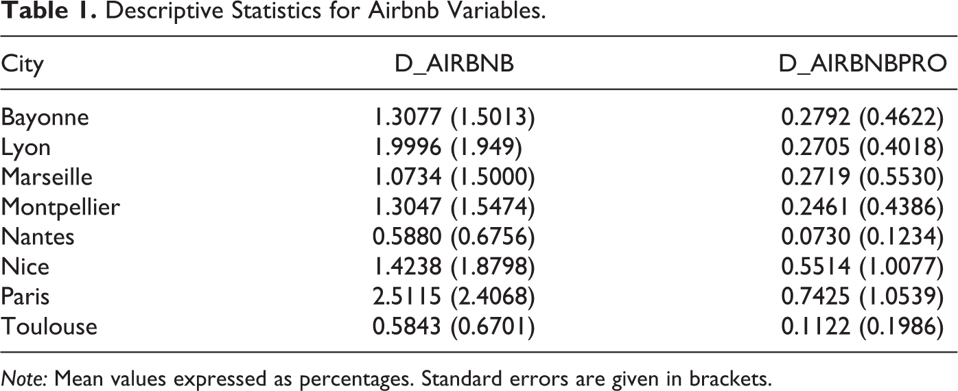
Note: Mean values expressed as percentages. Standard errors are given in brackets.

The greatest densities of Airbnb dwellings are in Paris (not surprisingly as it is the first worldwide destination in terms of the number of listings), Lyon, and Nice whereas the lowest ones are in Nantes and Toulouse. As can be seen from the correlation analysis we performed (see Online Appendix A2), there is a strong correlation between these two variables for all cities.

Private Sector Rental Variables

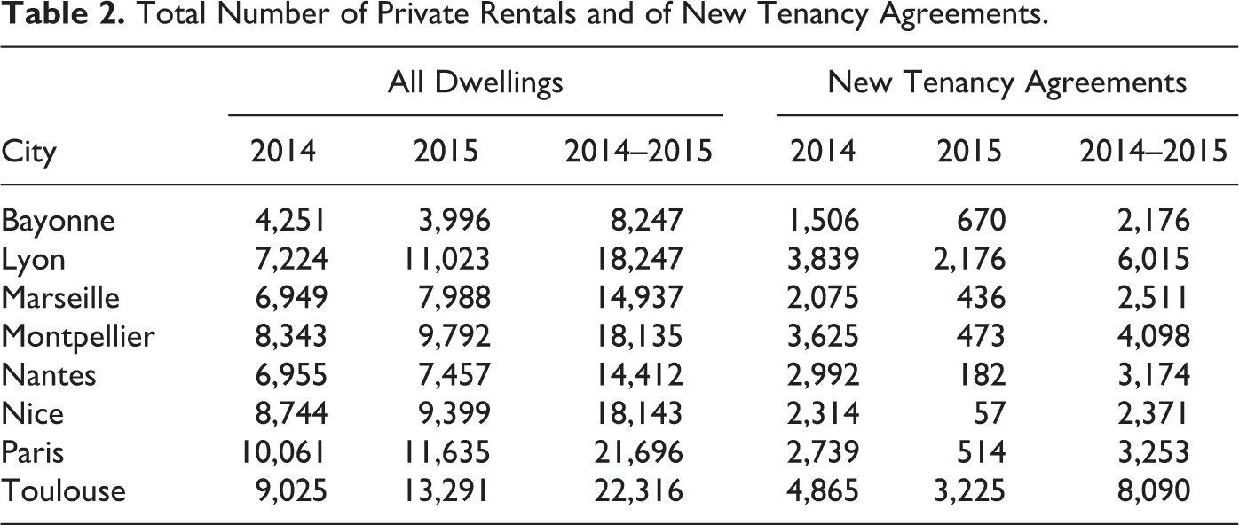
Data on private sector rents and structural characteristics of housing were obtained from a recently created network of French private rental market observatories, which aims at providing researchers and policy makers with high-quality detailed standardized rental microdata of dwelling characteristics for several areas in France. Table 2 provides, for each year and each city, the total number of private rentals including the number of new tenancy agreements. By new tenancies, we refer to the sample restricted to dwellings for which the “move-in” agreement was contracted in either 2014 or 2015.

Table 2.

Total Number of Private Rentals and of New Tenancy Agreements.

City	All Dwellings			New Tenancy Agreements
City	2014	2015	2014–2015	2014	2015	2014–2015
Bayonne	4,251	3,996	8,247	1,506	670	2,176
Lyon	7,224	11,023	18,247	3,839	2,176	6,015
Marseille	6,949	7,988	14,937	2,075	436	2,511
Montpellier	8,343	9,792	18,135	3,625	473	4,098
Nantes	6,955	7,457	14,412	2,992	182	3,174
Nice	8,744	9,399	18,143	2,314	57	2,371
Paris	10,061	11,635	21,696	2,739	514	3,253
Toulouse	9,025	13,291	22,316	4,865	3,225	8,090

Thanks to these data, we know for each dwelling: the rent excluding charges, the main structural characteristics, and the geographical coordinates. It is therefore possible to precisely characterize the environment of these dwellings by matching databases available at the IRIS or municipality scale.

To guarantee data confidentiality, the geographical coordinates of dwellings are scrambled by displacing them by a random direction (angle) and distance. More specifically, a buffer is drawn around each observation, then a point is selected randomly inside the buffer from a large number of randomly generated points. Used by Burgert et al. (2013) on data from demographic and health surveys, this method has been adapted to data produced by the rental market observatories. The radius of buffers varies with housing density of the private rental sector to guarantee the presence of thirty dwellings in each buffer. Therefore, the greater the housing density in the IRIS, the lower the maximum displacement distance in order to guarantee the same level of confidentiality whatever the housing density of the unit. Three constraints were also imposed: (i) the minimum displacement distance must be more than 20 meters to ensure a high level of confidentiality, (ii) the maximum displacement distance cannot exceed 250 meters to limit biases due to scrambling in very sparsely populated areas, and (iii) scrambled dwellings are positioned in the same IRIS as the original dwellings to ensure the quality of the match with socioeconomic data from the census. This bias may affect the properties of the estimators and the interpretation of the results by introducing an error into the measurement of distance variables (e.g., distance from dwellings to facilities) that may affect the properties of estimators (e.g., larger variances; Arbia, Espa, and Giuliani 2015). In addition, it partly modifies the assessment of spatial interdependence between rent levels.⁴

Our dependent variable is the monthly rent excluding charges measured at the survey date and expressed in euros. The database also provides for each dwelling the following structural characteristics: the type of dwelling (individual or collective), the building period (before 1946, between 1946 and 1970, between 1971 and 1990, between 1991 and 2005, after 2005), the type of management (direct or delegated), the surface area (m²), the average surface area per room (m²), and the tenant occupancy (in years). These variables are available for all cities. The floor on which the dwelling is located, the presence of an elevator, a concierge, or a parking space, the type of property (presence or not of common area maintenance charges), and the number of toilets and bathrooms are available and used for Paris only but not for the other cities. The entire set of variables is presented in Table 3, and Tables A3a to A3d in Online Appendix provide descriptive statistics for these structural variables by city for the complete sample.⁵

Table 3.

Rent Data and Structural Variables.

Label	Description	Source
RENT	Monthly rent excluding charges at the survey date (euros)	OL
HOUSTYPE	Type of dwelling (1: individual; 2: collective)	OL
BUILDPER	Building period (1: before 1946; 2: 1946–1970; 3: 1971–1990; 4: 1991–2005; 5: after 2005)	OL
MANAGTYPE	Type of dwelling management (1: delegated; 2: direct)	OL
SURFACE	Total surface area (m²)	OL
AVSUROOM	Average surface area per room (m²)	OL
TIMESPENT	Tenant occupancy (years)	OL
FLOOR	Floor	OLAP
ELEVATOR	Presence of an elevator (1: yes; 2: no)	OLAP
BUILDMANAG	Presence of a concierge (1: yes; 2: no)	OLAP
PROPTYPE	Presence of common area maintenance charges (1: no; 2: yes)	OLAP
PARKING	A parking space is included in the rent (1: yes; 2: no)	OLAP
NBTOIL	Number of toilets	OLAP
NBBATH	Number of bathrooms	OLAP

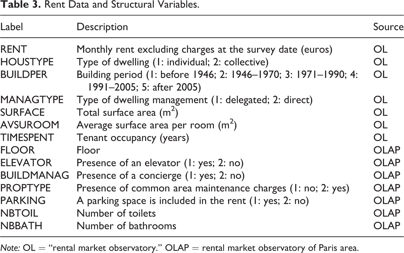
Note: OL = “rental market observatory.” OLAP = rental market observatory of Paris area.

Control Variables

The structural characteristics of dwellings are not the only factors explaining private sector rental levels. Many studies, mainly on real estate markets, show that the location of housing and the characteristics of its environment also impact housing prices. For example, in a review of the literature on households’ willingness to pay for different amenities, Gibbons and Machin (2008) identify several studies showing that school quality, proximity to transport infrastructures, and crime levels all play a key role in the formation of real estate prices. In the case of rent levels in the Brussels area, Bala, Peeters, and Thomas (2014) find a positive impact of median income, job accessibility, and environmental quality. Similarly, Efthymiou and Antoniou (2013), who focus on the effect of transport infrastructures and policies on the price of real estate and rents, show, in the case of Athens, that public transport increases rents, while the presence of large infrastructures like a port or an airport near the housing has a negative impact. Thus, in addition to the structural characteristics of dwellings, we construct a large set of variables to describe accessibility to jobs and services, socioeconomic context, and environmental quality around housing. Table 4 describes these additional control variables.

Table 4.

Control Variables.

Label	Description	Source	Scale	Date
Jobs and services accessibility
DIST_TRAMETR	Distance to the nearest tram or metro station (km)	Base ATC, CEREMA and local authorities in charge of public transport management	Dwelling	2015
NB_BUSSTOP	Number of bus stops in a 500-meter buffer	Base ATC, CEREMA and Local authorities in charge of public transport management	Dwelling	2015
SHOP_DENS	Density of shops (number/hectare)	BPE, INSEE	IRIS	2014 and 2015
HOTEL_DENS	Density of hotels (number/hectare)	Atout France—Agence de développement touristique de la France	IRIS	2013
DIST_CENTER	Distance to the city center (km)	GEOFLA®, IGN	Dwelling	2013
Environmental quality
DIST_ROAD	Distance to the nearest main road (km)	BD TOPO®, IGN	Dwelling	2013
DIST_RAILWAY	Distance to the nearest main railway (km)	BD TOPO®, IGN	Dwelling	2013
DIST_BUSIPARK	Distance to the nearest business park of more than 5 ha (km)	BD TOPO®, IGN	Dwelling	2013
DIST_COAST	Distance to the coast (km)	TCH HISTOLITT®, IGN-SHOM	Dwelling	2009
DIST_WATER	Distance to the nearest water area (waterway or water body; km)	BD TOPO®, IGN	Dwelling	2013
Socioeconomic context
SOCIALHOUS	Share of social housing (%)	RP, INSEE	IRIS	2013
OWNERS	Proportion of owner-occupiers (%)	RP, INSEE	IRIS	2013
SECONDHOME	Share of second homes (%)	RP, INSEE	IRIS	2013
STUDENT	Share of students (%)	RP, INSEE	IRIS	2013
WORKERS	Share of workers (%)	RP, INSEE	IRIS	2013
EXECUTIVES	Share of executives (%)	RP, INSEE	IRIS	2013
IMMIGRANTS	Share of immigrants (%)	RP, INSEE	IRIS	2013
UNEMPLOY	Unemployment rate of fifteen- to sixty-four-year olds (%)	RP, INSEE	IRIS	2013
INCOME	Median income (euros)	RFLM, INSEE-DGFiP	IRIS	2011
HONOURATE_PU	Honor rate at Brevet of the nearest public junior high school (%)	MENESR-DEPP	Dwelling	2014 and 2015
HONOURATE_PR	Honor rate at Brevet of the nearest private junior high school (%)	MENESR-DEPP	Dwelling	2014 and 2015
DIST_ZUS	Distance to the nearest deprived neighborhood (km)	CGET	Dwelling	2015

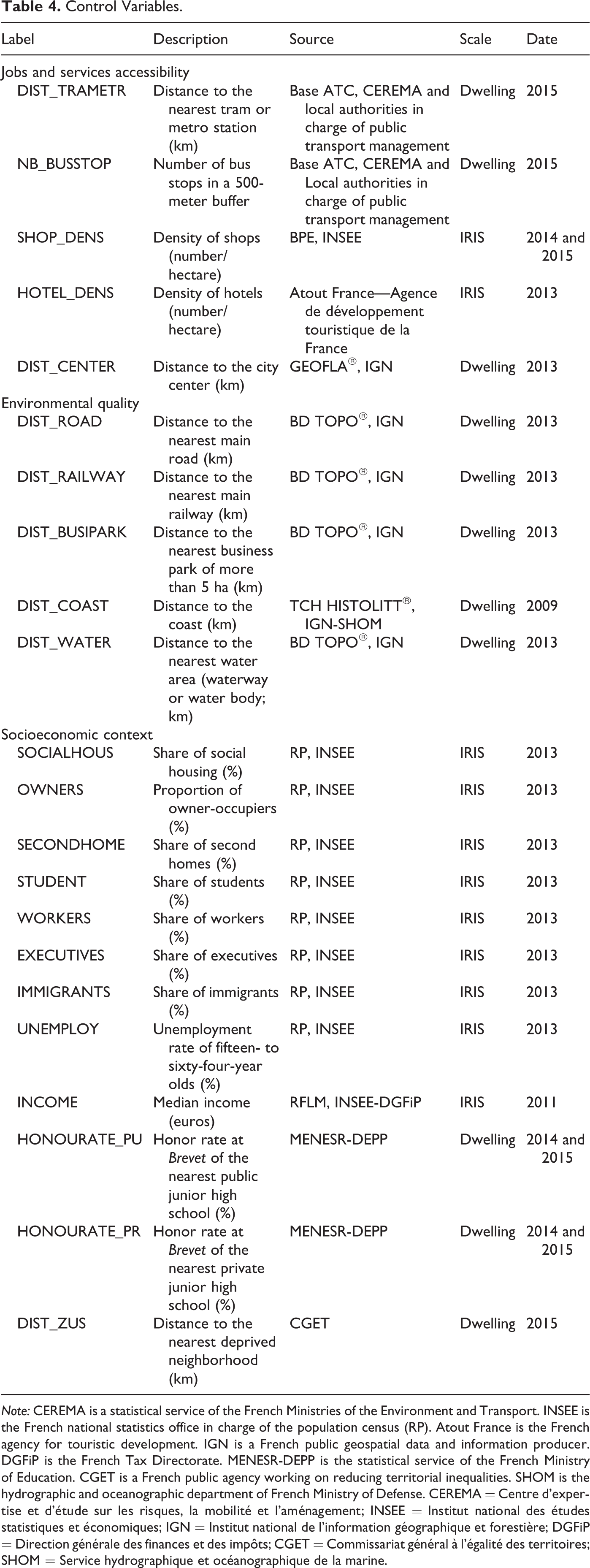
Note: CEREMA is a statistical service of the French Ministries of the Environment and Transport. INSEE is the French national statistics office in charge of the population census (RP). Atout France is the French agency for touristic development. IGN is a French public geospatial data and information producer. DGFiP is the French Tax Directorate. MENESR-DEPP is the statistical service of the French Ministry of Education. CGET is a French public agency working on reducing territorial inequalities. SHOM is the hydrographic and oceanographic department of French Ministry of Defense. CEREMA = Centre d’expertise et d’étude sur les risques, la mobilité et l’aménagement; INSEE = Institut national des études statistiques et économiques; IGN = Institut national de l’information géographique et forestière; DGFiP = Direction générale des finances et des impôts; CGET = Commissariat général à l’égalité des territoires; SHOM = Service hydrographique et océanographique de la marine.

Accessibility variables

We use three databases to describe accessibility to different amenities: the Base permanente des équipements (BPE) of INSEE for the years 2014 and 2015, the Base nationale des arrêts de transport (Base ATC) produced by CEREMA for 2015, and a database produced by Atout France for 2013.

The BPE is used to describe the presence of shops near the housing (SHOP_DENS). More specifically, we calculate a shop density (expressed as the number of shops per hectare) at the IRIS scale. These data, available for 2014 and 2015, are matched with rent data for the corresponding years. To capture the effect of touristic attractiveness on rents, we compute the density of hotels (HOTEL_DENS) of the IRIS using a database from Atout France, which provides the precise geolocation of hotels.

The Base ATC produced by CEREMA provides geolocated data on public transport stations (train stations, tram and metro stations, and bus stops). It is produced by local authorities in charge of public transport management and distributed by CEREMA after various improvements in data consistency. For each dwelling, we calculate Euclidean distances to the nearest metro or tram station (DIST_TRAMETR). As bus stops cover cities much more densely, we build a different variable by summing the bus stops located within a 500-meter radius of dwellings (NB_BUSSTOP). Note that the distances to the nearest metro or tram station and bus stop are only computed for cities with such facilities and for which data were available.

Finally, to capture proximity to the main centers for services and jobs, we calculate a Euclidean distance between each dwelling and the municipality center. We follow the Institut national de l’information géographique et forestière (IGN) definition (i.e., the main French geospatial data producer) to identify the municipality center. By this definition, it is located at the center of the building block containing the city hall.

Environmental quality variables

To capture the effect of environmental amenities or disamenities on rents, we use two sources: BD TOPO® produced by IGN and the HISTOLITT® database jointly produced by IGN and SHOM.

The BD TOPO® provides a three-dimensional vectorial description of the elements of the territory and its infrastructures. This database covers all geographical and administrative entities of the national territory to the nearest meter. We use it to compute the distance between housing and infrastructures or facilities that may generate nuisances and pollution and adversely affect rents. For this study, we consider main roads and railways as well as business parks. We compute the Euclidean distances between each dwelling and the nearest point located on the route of a railway (DIST_RAILWAY) or road (DIST_ROAD) and between each dwelling and the nearest point located on the perimeter of a business park (DIST_BUSIPARK).

We also use the BD TOPO® to build one variable related to the presence of landscape amenities: the effect of the proximity to a waterway or a water body on rents. We compute the Euclidean distance between each dwelling and the perimeter of the nearest water area (DIST_WATER).

Finally, for coastal cities we estimate, using the HISTOLITT® database, a Euclidean distance between each dwelling and the coastline (DIST_COAST) in order to capture the effect of proximity to the seafront on rents. Montpellier, Nice, Marseille, and Bayonne are considered to be coastal cities. This variable is therefore not included in the econometric regressions for the other cities.

Socioeconomic context variables

Various variables were also constructed to reflect the socioeconomic context of the dwellings’ neighborhood.

INSEE census data for 2013 are used to characterize the housing stock with the following variables: the share of social housing (SOCIALHOUS), the share of second homes (SECONDHOME), and the proportion of owner-occupiers (OWNERS). We also construct different variables to describe the sociodemographic composition of the resident population: the share of manual workers (WORKERS) and executives (EXECUTIVES), the unemployment rate of fifteen- to sixty-four-year-olds (UNEMPLOY), and the share of immigrants (IMMIGRANTS) and students (STUDENT) in the total population. To supplement these variables, we use data from Dispositif Revenus Localisés produced jointly by INSEE and DGFiP for the year 2011 to compute the median income of consumption units (INCOME). All these variables are available at the IRIS scale.

In France, since 1996, urban and social policies have focused on deprived areas, initially defined by public policies as Zones urbaines sensibles (ZUS) and more recently as “quartiers prioritaires.” In order to take into account the effect of this public policy on rents, we compute the Euclidean distance between each dwelling and the perimeter of the nearest deprived neighborhood (DIST_ZUS) based on a digital map provided by Commissariat général à l’égalité des territoires.

Furthermore, the statistical services of the French Ministry of Education provide geolocalized data on public⁶ and private junior high school performances for the years 2014 and 2015. In France, because of a residence-based assignment policy (Carte scolaire), parents are not free to choose the public school their children attend. In order to assign each pupil to a public school, catchment areas are defined using the precise address of pupils. Because of the lack of geographic information system (GIS) data on catchment areas, we identify the nearest public and private schools for each dwelling and assign the performance indicators of these schools to the dwellings. We thus obtain two different variables: the honor rate at the final exam (Brevet des collèges) for junior public (HONOURATE_PU) and private (HONOURATE_PR) high schools. These data, available for 2014 and 2015, are matched with rent data for the corresponding years. Tables in Online Appendix A4 provide descriptive statistics for the additional control variables used.

Exploratory Analysis of Airbnb Data and Estimation Results

In this section, we first provide some descriptive statistics pertaining to the evolution of the Airbnb activity for our sample. Then, we turn to the estimation results.

Exploratory Analysis of Airbnb Data

From the monthly file, we report in Table 5 the evolution, by city, of the total number of dwellings that have been booked at least one time in the month. Globally, we observe a sustained growth of the activity of Airbnb, although differences arise according to the city. Growth was particularly high in the coastal city of Bayonne and in the major cities of Marseille and Toulouse. It was lower in Strasbourg, Nice, and Lyon. There is also some seasonality, as shown in figure in Online Appendix A5 that displays the monthly change in occupation rate by city over the period. Peaks of occupation rates around 60 percent are typically observed in August for most cities while they are around 20 percent during the winter months. In some other cities (Nantes, Paris, Toulouse), occupation rates do not display seasonal variations.

Table 5.

Changes in Airbnb Listings for the Cities under Study.

City	Number of Listings
City	10/2014 to 12/2014	2015	2016^a
Bayonne	529	7,254	17,793
Lyon	3,154	21,426	46,825
Marseille	1,807	17,487	41,045
Montpellier	1,059	11,114	23,229
Nantes	591	5,796	13,304
Nice	1,939	22,760	43,823
Paris	29,510	193,178	235,126
Toulouse	1,032	9,199	22,175
Total	39,621	288,214	443,320

^a For Paris, the ads have not been collected beyond September 2016.

In the monthly file, the number of announcers is 109,983 while the number of ads is 136,763. Some announcers therefore own several dwellings. Table 6 provides, for each city and each year, the number and the share of Airbnb dwellings of professional nature according to our definition. It also displays the mean and maximum number of Airbnb dwellings per owner (the median being 1 in all cities). Large disparities can be observed depending on the location. For instance, the share of professional activity is less frequent in Lyon (10.6 percent in 2014 and 18.4 percent in 2016) while it reaches 45.2 percent in 2014 and 40.1 percent in 2016 in Nice. The mean and maximum numbers of dwellings per owner increased between 2014 and 2016. The maximum values (194 in Paris and 97 in Bayonne in 2016) clearly show that professional advertisers organize a rental system comparable to hotel activities.

Table 6.

Distribution of Professional and Private Individual Dwellings.

		Number of Airbnb Dwellings		Share of Professional Airbnb Dwellings (%)	Number of Airbnb Dwellings per Owner
City	Year	Pro.	Priv.	Share of Professional Airbnb Dwellings (%)	Mean	Max
Bayonne	2014	90	195	31.6	1.42	5
	2015	552	1,597	25.7	2.11	19
	2016	1,297	3,006	30.1	4.95	97
Lyon	2014	198	1,663	10.6	1.50	16
	2015	721	5,106	12.4	1.7	26
	2016	2,143	9,526	18.4	2.03	70
Marseille	2014	224	683	24.7	1.31	7
	2015	885	3,349	20.9	1.87	30
	2016	2,263	7,506	23.2	2.01	34
Montpellier	2014	118	400	22.8	1.37	5
	2015	530	2,370	18.3	2.11	40
	2016	1,316	4,444	22.8	2.74	71
Nantes	2014	39	243	13.8	1.20	4
	2015	176	1,180	13.0	1.29	5
	2016	563	2,295	19.7	1.42	13
Nice	2014	457	555	45.2	3.72	44
	2015	2,012	3,173	38.8	4.13	63
	2016	3,911	5,837	40.1	5.07	83
Paris	2014	4,849	9,053	34.9	2.79	82
	2015	11,807	36,183	24.6	4.84	173
	2016	21,723	44,473	32.8	5.19	194
Toulouse	2014	130	364	26.3	2.25	16
	2015	466	1,845	20.2	3.18	49
	2016	1,125	4,460	20.1	2.69	60

The table in Online Appendix A6 provides some additional insights to characterize the differences between private and professional owners. In general, the response rate is higher and the response time is lower for professional advertisers. The latter also use more instant booking.

Estimation Results

We estimate the following equation for each city:

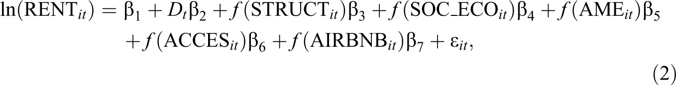
ln ({RENT}_{i t}) = β_{1} + D_{t} β_{2} + f ({STRUCT}_{i t}) β_{3} + f (SOC_{ECO}_{i t}) β_{4} + f ({AME}_{i t}) β_{5} + f ({ACCES}_{i t}) β_{6} + f ({AIRBNB}_{i t}) β_{7} + ∊_{i t},

where the dependent variable is expressed in logarithms; D_t, ${STRUCT}_{i t}$ , ${SOC_ECO}_{i t}$ , ${AME}_{i t}$ , ${ACCES}_{i t}$ , and ${AIRBNB}_{i t}$ represent the vectors of time dummies, structural (including the surface area), economic, amenity, accessibility, and Airbnb variables, respectively. While the same set of socioeconomic variables is included for each city, the selection of the accessibility and (dis)amenity variables is city specific. Indeed, these variables measure very localized effects, such as the proximity to a major road or distance to the coast, so that it is not relevant to introduce all of them for all cities. Therefore, we kept only those variables that best explain the variability of rents while avoiding multicollinearity by applying a tolerance threshold of 5 for the VIF measure. In addition, we test for each city the need to integrate all the variables expressed as distances in splines up to order 3 as most economic relationships are detectable at this order. If the use of splines proves to be irrelevant, we introduce the variable in level in our estimates.

For the estimation of the SHAC variance–covariance matrix,⁷ we use a Parzen kernel. This function takes as an argument the spatio-temporal distance matrix described in Online Appendix 1 and returns a variance–covariance matrix. Note that the Parzen kernel is used with a threshold distance of 250 meters, that is, dwellings separated by more than 250 meters are considered as not interacting.⁸ The further apart two dwellings are, the less the weight associated in the variance–covariance matrix. In order to avoid having dwellings interacting only with themselves, we remove from our starting base, and for each city, all the dwellings that do not have neighbors within a 250-meter radius. Table 7 shows the number of observations for each city before and after pruning, when all the observations are included and when only the new tenancy agreements are included. This procedure results in the loss of a relatively small number of observations.

Table 7.

Number of Observations before and after Pruning for All Observations and for the Sample Restricted to the New Tenancy Agreements.

City	All Observations			New Tenancy Agreements
City	Nb. Obs	Nb. Obs after NA Removal	Nb. Obs after Pruning	Nb. Obs	Nb. Obs after NA Removal	Nb. Obs after Pruning
Bayonne	8,247	8,221	8,183	2,176	2,167	2,120
Lyon	1,8247	18,093	18,079	6,015	5,991	5,960
Marseille	14,937	14,803	14,660	2,511	2,486	2,264
Montpellier	18,135	18,094	18,078	4,098	4,096	4,053
Nantes	14,412	14,412	14,389	3,174	3,174	3,101
Nice	18,143	18,131	18,081	2,371	2,369	2,315
Paris	21,696	21,584	21,563	3,253	3,234	3,126
Toulouse	22,316	22,316	22,266	3,174	3,174	3,101

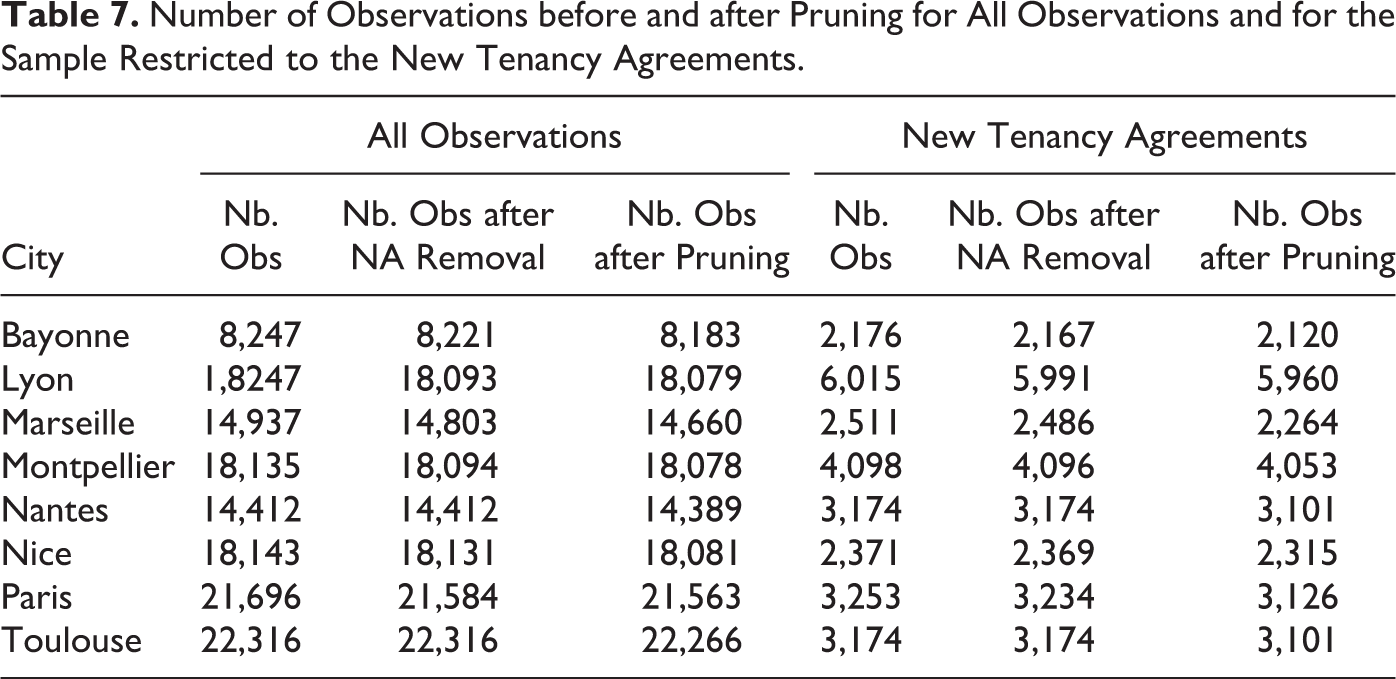
Table 8 displays the quality of adjustment of the estimations for each city, measured by the coefficient of determination and its adjusted version to take account of the varying number of variables for each city. The variables included in the specification explain a significant part of the variance in rent levels and thus constitute major determinants of the formation of rent levels in cities. For the whole sample, the largest adjusted coefficient of determination is obtained for Paris, with more than 90.9 percent of the variance of the rent levels explained and the lowest, but still with a satisfactory level of 64.4 percent of the variance explained, is obtained from the estimates made for Marseille. We now turn to the analysis of the impact of the various categories of variables on rents, first, the control variables and, second, the variables of interest.

Table 8.

Quality of Adjustment by City for All Observations and for the Sample Restricted to the New Tenancy Agreements.

City	All Observations		New Tenancy Agreements
City	R ²	Adjusted R ²	R ²	Adjusted R ²
Bayonne	.6530	.6518	.7396	.7361
Lyon	.7977	.7972	.8299	.8289
Marseille	.6444	.6436	.7080	.7041
Montpellier	.7960	.7955	.8741	.8727
Nantes	.8269	.8263	.8103	.8074
Nice	.7817	.7813	.9209	.9197
Paris	.9092	.9090	.8062	.8053
Toulouse	.7674	.7671	.7080	.7041

Impact of the control variables

We first provide a quick description of the effects of the control variables. The estimation results are presented graphically to make it easier to compare the values of the determinants of private sector rental levels among cities. The corresponding graphs are provided in Online Appendix 2, in particular the complete estimation results, obtained for the whole sample,⁹ are in Table A13.

As regards the impact of the structural variables, the results first show that the effect of the surface area is nonlinear (the coefficients of the spline function being significant). However, it remains broadly constant with the increase in housing size (see Online Appendix, Figure A8). Figure A9 in Online Appendix provides a graphical representation of the effects of the other variables. Housing built during the period 1946–1970 (reference period) is the least valued by households everywhere except in Nice and Bayonne where the dwellings built before 1946 are valued even less. This effect is expected since the period 1946–1970 corresponds to massive constructions of large sets of collective housing, mostly judged of poor quality and inducing relatively high rental charges, such as heating. By contrast, dwellings built before 1946 generally have a sought-after architecture (e.g., Haussmann style apartments in Paris). From 1971 onward, we also see that the more recent housing is, the more it is valued for all cities. This reflects a rise in terms of equipment and comfort. Overall, these results are consistent with those of previous studies conducted in the Bordeaux conurbation (Décamps and Gaschet 2013) and Angers (Travers, Appéré, and Larue 2013) for the real estate markets or in Paris (Prandi and Moumouni 2014) for the private rental sector. As regards the other structural determinants, the time spent in the dwelling has a significant and negative impact on rental levels everywhere. This result is explained by the frequent upward revaluation of rent levels carried out by landlords when tenants change. The effect of this variable is strongest in Paris where the high strain on the housing market contributes to strong upward pressure on rents. The coefficient associated with the average surface area per room is significant and negative everywhere, reflecting the fact that households value more rooms for the same surface area. In addition, compared to delegated management, direct management of housing is associated with higher or at least equivalent rent.

These results can be refined by introducing additional structural variables for Paris (see Online Appendix, Table A13). The estimated coefficients of the floor variables indicate that the dwellings located on the ground floor (which is the reference modality) are the least valued as expected because of the greater exposure to burglary and the associated negative externalities (noise, passersby, etc.), whereas the fifth floor is the most highly valued. The variables relating to the comfort of dwellings (presence of an elevator or parking space and the number of toilets) have the expected effects and are significant, with the exception of the number of bathrooms, which is not significant. The presence of a caretaker has a negative effect, which can be explained by the fact that the tenant thinks “all charges included” and accepts a higher rent as the charges will be low, as Prandi and Moumouni (2014) interpret it for individual heating. Finally, dwellings with common area maintenance charges are associated with higher rents without charges.

For socioeconomic variables (see Online Appendix, Figure A10), we note that the proportion of owner-occupiers in the IRIS, when significant, negatively affects rent levels: a strong presence of owner-occupiers more often characterizes the residential housing districts that are less valued after. The income variable, as expected, has a positive and significant effect on the rent levels in most cities. The distance from the dwelling to the priority neighborhood of the city’s policy is insignificant everywhere. The share of manual workers, which is frequently used (in conjunction with those in higher education and higher learning professions) to analyze the social differentiation of urban spaces, has a negative and significant effect in Nice and Paris only. Moreover, the performance of schools, measured by the honor rate at Brevet of public junior high schools, has a positive effect on rents, but this is significant for the cities of Paris, Montpellier, Toulouse, and Marseille only (and also for private schools for the latter). The share of social housing in the IRIS has a positive effect on rental levels in Nantes and Toulouse only and is insignificant elsewhere. Finally, the other socioeconomic variables included in the estimates show more nuanced results. For instance, the share of second homes, an indicator of tourist attractiveness, is driving up rents in Paris, Nantes, Toulouse, and Nice and driving down rents in Marseille. The share of students and the share of immigrants are rarely significant.

With respect to the accessibility variables (see Online Appendix, Figure A11a), distance to the city center usually reduces rents, except in Bayonne and somewhat in Nice, where rents increase with the distance beyond 1.5 km (respectively 4 km). The pressure of tourism in these two coastal cities probably explains the higher rents with the distance to the center of the city. The other accessibility variables (Figure A11b) are more rarely significant. The density of hotels has a positive impact in Nantes.

With respect to amenities/disadvantages (see Online Appendix, Figure A12), it appears that the proximity to a major road does not impact rents, except in Paris and Nice where the impact is positive. The effects of proximity to a railway and the distance to the water area are only significant and positive in Lyon.

Impact of Airbnb rentals

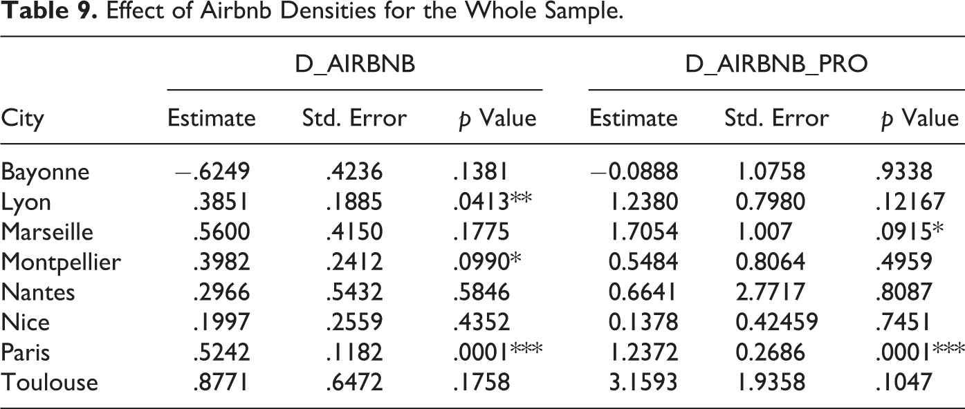
We report in Tables 9 and 10 the estimated coefficients for our two Airbnb variables D_AIRBNB and D_AIRBNBPRO, first for the whole sample and second for the sample restricted to the new tenancy agreements. As mentioned before, both variables are strongly correlated. Therefore, we have estimated two specifications in order to include them separately. The first one includes the density of all Airbnb housing in the IRIS. The second one includes only the density of professional Airbnb housing in the IRIS. For ease of interpretation, we report here the transformed coefficients in these tables, in order to obtain a percentage interpretation directly, in other words, as our base specification is a semilog model, we have multiplied all coefficients and corresponding standard errors by 100.

Table 9.

Effect of Airbnb Densities for the Whole Sample.

City	D_AIRBNB			D_AIRBNB_PRO
City	Estimate	Std. Error	p Value	Estimate	Std. Error	p Value
Bayonne	−.6249	.4236	.1381	−0.0888	1.0758	.9338
Lyon	.3851	.1885	.0413**	1.2380	0.7980	.12167
Marseille	.5600	.4150	.1775	1.7054	1.007	.0915*
Montpellier	.3982	.2412	.0990*	0.5484	0.8064	.4959
Nantes	.2966	.5432	.5846	0.6641	2.7717	.8087
Nice	.1997	.2559	.4352	0.1378	0.42459	.7451
Paris	.5242	.1182	.0001***	1.2372	0.2686	.0001***
Toulouse	.8771	.6472	.1758	3.1593	1.9358	.1047

Table 10.

Effect of Airbnb Densities for the Restricted Sample of New Tenancy Agreements.

City	D_AIRBNB			D_AIRBNB_PRO
City	Estimate	Std. Error	p Value	Estimate	Std. Error	p Value
Bayonne	0.0936	0.8958	.9164	0.7140	3.3000	.8265
Lyon	0.2386	0.2637	.3654	1.2928	1.0465	.2173
Marseille	1.3040	0.9215	.1578	6.4641	3.5239	.0705*
Montpellier	2.9960	0.5895	.0001***	7.9153	1.7208	.0001***
Nantes	−2.3485	2.2767	.2911	−10.2137	7.2313	.1228
Nice	−1.1637	1.3628	.3872	−1.8658	1.9808	.3369
Paris	1.3537	0.3661	.0002***	1.7083	0.7106	.0167**
Toulouse	0.7402	0.5954	.2141	1.7713	1.9121	.3539

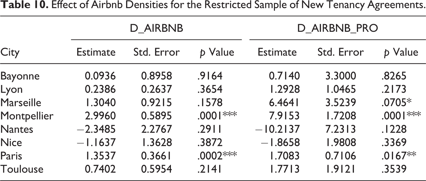
For the whole sample, the Airbnb rentals density significantly impacts private-sector rental levels for Lyon, Paris, and Montpellier only. An increase in the Airbnb rental density by one point at the IRIS level leads to an increase in private rental levels of 0.3851 percent, 0.3982 percent, and 0.5242 percent, respectively, in Lyon, Montpellier, and Paris. When focusing on the density of professional Airbnb rentals, the effect remains highly significant for Paris but becomes insignificant for Lyon and Montpellier and significant for Marseille. Thus, a one-point increase in the density of professional Airbnb rental units at the IRIS level leads to an increase in private-sector rental levels of, respectively, 1.7054 percent and 1.2372 percent in Marseille and Paris. The coefficients are even larger when we restrict the sample to the new tenancy agreements: a one-point increase in the Airbnb rental density at the IRIS level leads to an increase in private-sector rental levels of 2.996 percent and 1.3537 percent in Montpellier and Paris, respectively, while it rises to 6.4641 percent, 7.9153 percent, and 1.7083 percent for an increase in the density of professional housing in Marseille, Montpellier, and Paris, respectively. When significant, the impact is therefore much higher for the new tenancy agreements: owners tend to reevaluate more significantly the level of the rent for new renters in the most strained cities in our sample. Although we observe some slight changes in the set of cities with significant coefficients according to the definition of the density (D_AIRBNB vs. D_AIRBNBPRO) and the sample (whole sample vs. new tenancy agreements), Paris emerges as the city where there is always a significant effect of Airbnb rentals on private rents.

We have investigated the potential for heterogeneous impacts on rental rents of the Airbnb variables by having them interact with other variables capturing various aspects of the housing market in each IRIS, namely the proportion of owner-occupiers, the density of hotels, and the share of second homes. Note that the marginal effect of the Airbnb activity (D_AIRBNB and D_AIRBNBPRO) in the whole sample and in the restricted sample is significant for some values of each of these variables in Paris. In the other cities, the marginal effect of the Airbnb activity is only significant in Montpellier (for both D_AIRBNB and D_AIRBNBPRO) in the restricted sample and for some values of our variables of interest.

Specifically, in Paris, the marginal effects of both D_AIRBNB and D_AIRBNBPRO are significant, positive, and increasing for areas with “high” ownership rates (approximately 20 percent and beyond in the whole sample and approximately 25 percent and beyond in the restricted sample). They are displayed in Figure 2A–D.¹⁰ The effect of Airbnb then becomes larger in IRIS with high owner-occupancy rate and as reported previously, when significant, the effect is much greater for new tenancy agreements (restricted sample). The effect of Airbnb then becomes larger in IRIS with high owner-occupancy rate and as reported previously, when significant, the effect is much greater for new tenancy agreements (restricted sample). As our results earlier showed that, ceteris paribus, the proportion of owner-occupiers in the IRIS had a negative effect on rent levels, this new result implies that in fact, rents are more likely to increase for zones with increasing proportions of owner-occupiers (less attractive, with relatively low initial levels of rents) than in the other zones with greater initial levels of rents. This result contradicts the results obtained by Barron et al. (2017) for a sample of 492,000 observations for the period 2011–2015 at the zipcode level. However, unlike Barron et al.’s results, our sample is restricted to city centers where owners frequently rent their whole properties for tourism purposes.

Figure 2.

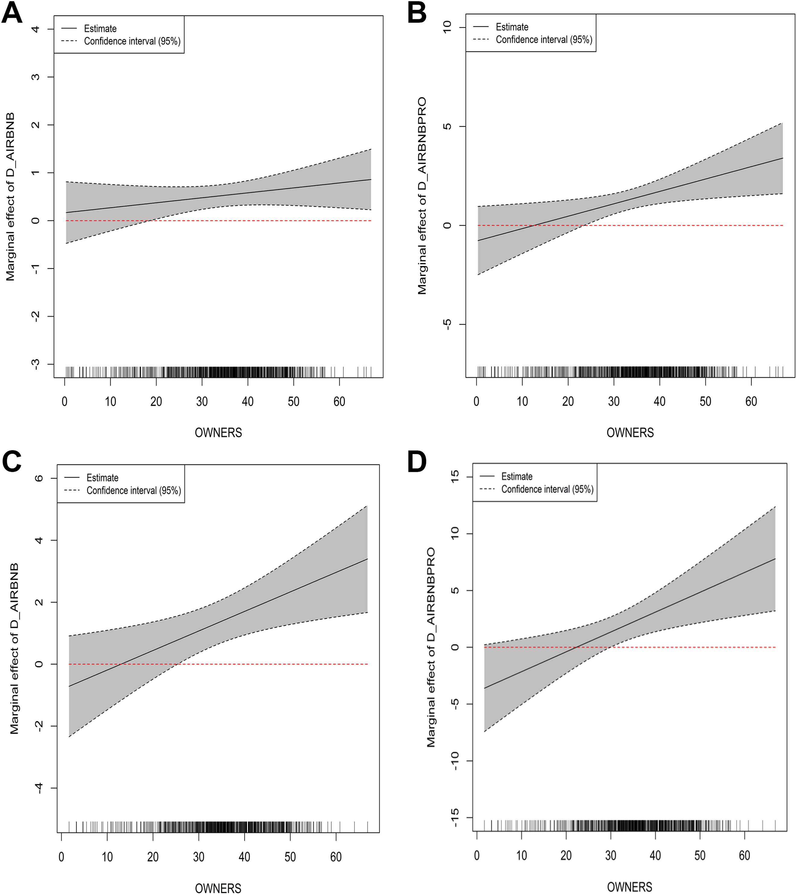
Marginal effect of Airbnb density on rental prices versus the proportion of owner-occupiers in Paris. (A) Whole sample, D_AIRBNB, (B) whole sample, D_AIRBNBPRO, (C) restricted sample, D_AIRBNB, and (D) restricted sample, D_AIRBNBPRO.

In the other cities, the marginal effect of the Airbnb activity is only significant in Montpellier (for D_AIRBNB whatever the rate and for D_AIRBNBPRO for rates of ownership from 20 percent) in the restricted sample. The corresponding changes in marginal effects are displayed in Figure 3A and B. Since the marginal effects are positive and increasing with the rate of ownership, the conclusions for Paris apply.

Figure 3.

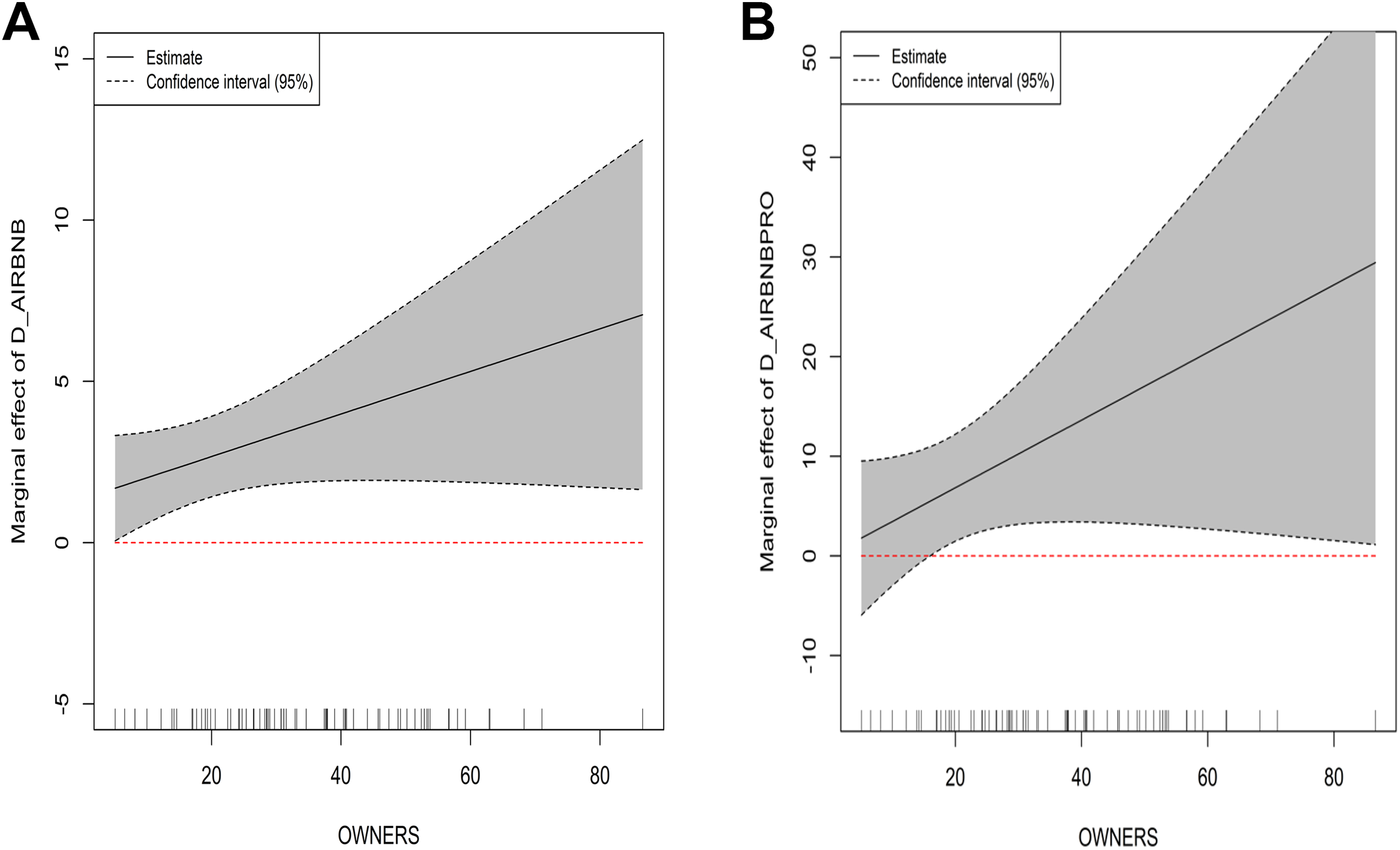
Marginal effect of Airbnb density on rental prices versus the proportion of owner-occupiers in the city of Montpellier. (A) Restricted sample, D_AIRBNB and (B) restricted sample, D_AIRBNBPRO.

For the share of second homes, in Paris, the marginal effects of both D_AIRBNB and D_AIRBNBPRO are significant and positive, but they decrease with the share of second homes up to approximately 15–20 percent (most of our observations are located in IRIS with less than 20 percent of second homes) in both the whole sample and the restricted sample. The corresponding changes in marginal effects of Airbnb density on rental prices depending on the value of the share of second homes are displayed in Figure 4A–D. The effect of Airbnb decreases with the share of second homes and even becomes nonsignificant with high rates of second homes. In areas with a high share of second homes, the Airbnb activity has no impact on private rental prices. Here also, when significant, the effect is much greater for new tenancy agreements.

Figure 4.

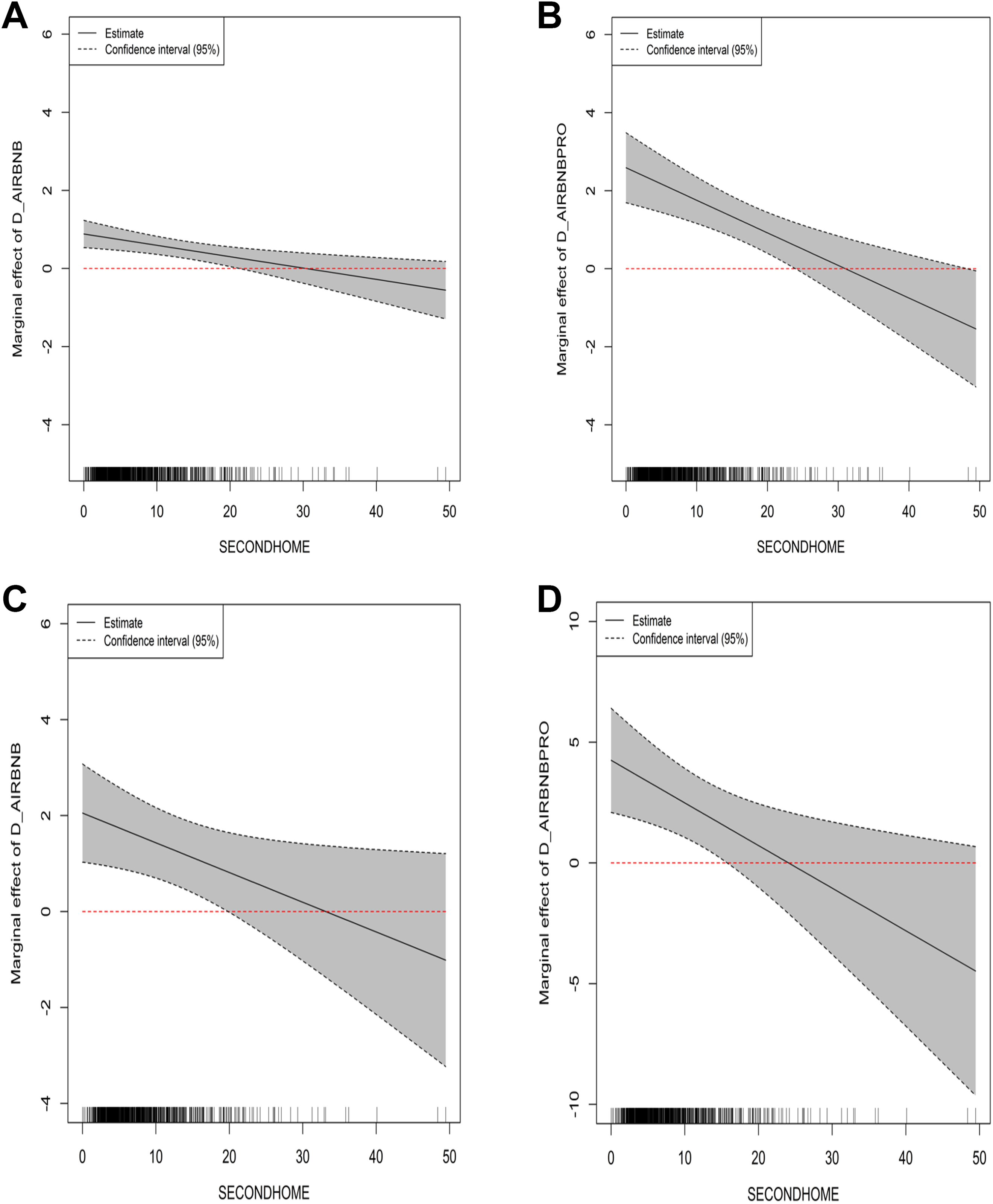
Marginal effect of Airbnb density on rental prices versus the share of second homes in Paris. (A) Whole sample, D_AIRBNB, (B) whole sample, D_AIRBNBPRO, (C) restricted sample, D_AIRBNB, and (D) restricted sample, D_AIRBNBPRO.

Apart from Paris, the marginal effect of the Airbnb activity is significant in Montpellier only (for both D_AIRBNB and D_AIRBNBPRO for almost all levels of share of second homes) in the restricted sample. The corresponding changes in marginal effects are displayed in Figure 5A and B. Unlike Paris, the marginal effects are positive and increasing with the share of second homes. Contrary to Paris, the higher the share of second homes in Montpellier, the stronger the pressure Airbnb exerts on rents.

Figure 5.

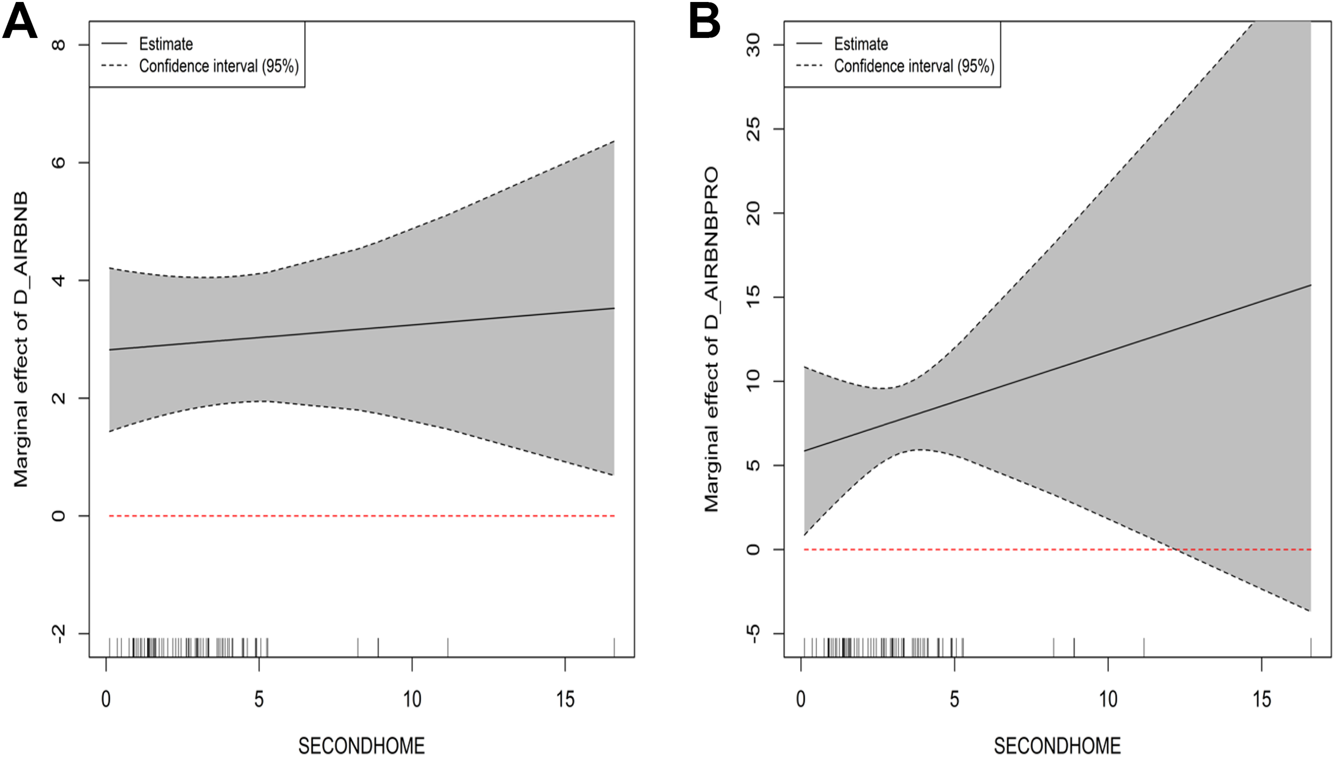
Marginal effect of Airbnb density on rental prices versus the share of second homes in Montpellier. (A) Restricted sample, D_AIRBNB and (B) restricted sample, D_AIRBNBPRO.

We finish with the “density of hotels” variable. It can be observed that in Paris, the marginal effects of both D_AIRBNB and D_AIRBNBPRO are significant, positive, and decreasing with the level of hotel density, up to approximately 1 for the whole sample and up to 0.5–1 for the restricted sample (here also, most of our observations are in IRIS with a density of hotels of less than 1). The corresponding changes in the marginal effects of Airbnb density on rental prices depending on the level of hotel density are displayed in Figure 6A–D. The effect of Airbnb decreases with the density of hotels and even becomes nonsignificant with a high density of hotels; and when significant, the effect is more important for new tenancy agreements. This would mean that areas with a high density of hotels are the most attractive ones in Paris (the level of rents in these areas is already relatively high).

Figure 6.

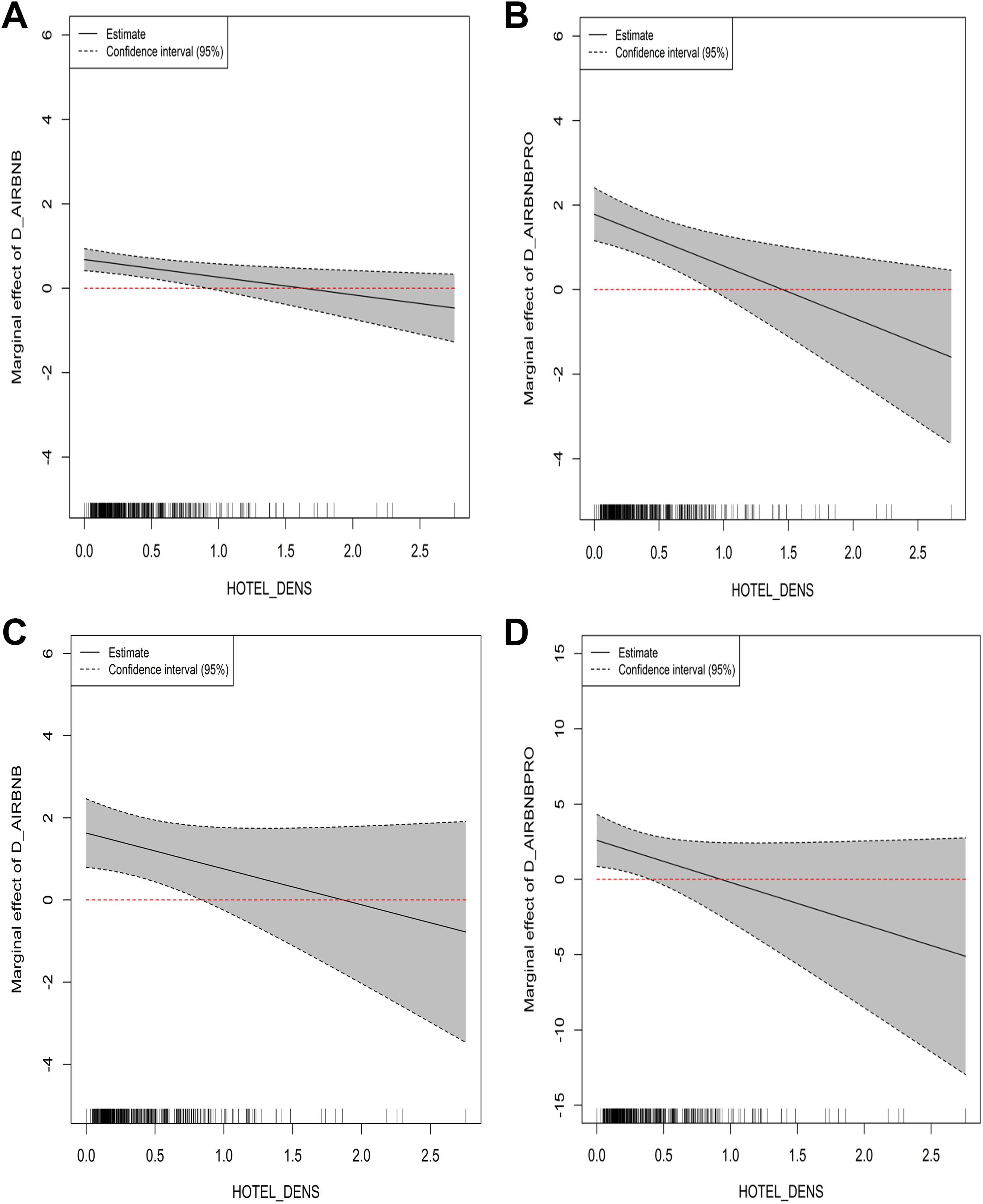
Marginal effect of Airbnb density on rental prices with respect to the density of hotels in Paris. (A) Whole sample, D_AIRBNB, (B) whole sample, D_AIRBNBPRO, (C) restricted sample, D_AIRBNB, and (D) restricted sample, D_AIRBNBPRO.

In the other cities, the marginal effects with respect to hotel density of the Airbnb activity are significant in Montpellier only (for both D_AIRBNB and D_AIRBNBPRO) in the restricted sample. The corresponding changes in marginal effects are displayed in Figure 7A and B. Since the marginal effects are positive and decreasing with the density of hotel, the conclusions for Paris apply.

Figure 7.

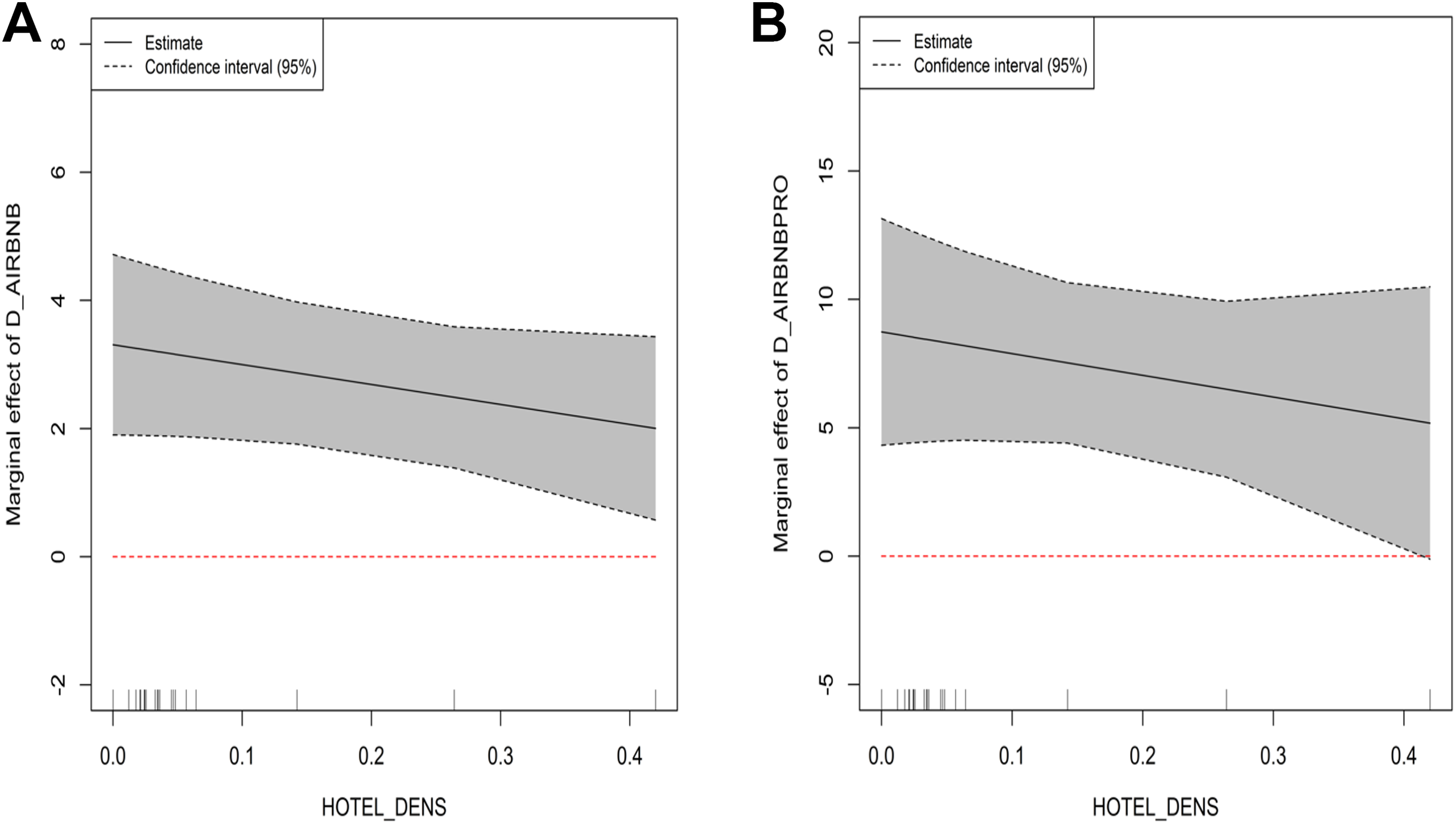
Marginal effect of Airbnb density on rental prices versus the density of hotels in Montpellier. (A) Restricted sample, D_AIRBNB and (B) restricted sample, D_AIRBNBPRO.

Globally, these results are consistent with those obtained in previous studies that all find a positive effect of Airbnb activities on rents or house prices. For example, Barron et al. (2017) using panel data of about 450,000 observations for the whole United States at the zipcode level between mid-2012 and the end of 2016 conclude that a 10 percent increase in Airbnb listings leads to a 0.42 percent increase in rents and 0.76 percent in house prices. Horn and Merante (2017), using panel micro data on 113,409 dwellings in the Boston area, find that a 1 standard deviation increase in Airbnb density leads to a 0.4 percent increase in local rents. They also show that the effect is higher with two or three bedrooms listings and not significant with studio or one bedroom listings. Sheppard and Udell (2018), using data on individual sales in the New York area (about 760,000 observations between January 2003 and August 2015), show that an increase of 100 percent in the number of Airbnb properties around the sales (300 meters) is associated with an increase of 6–9 percent depending of the specifications. Other papers provide estimates for aggregate spatial units. Based on a sample composed of web-scraped information on Airbnb listings in Barcelona and rent data at the neighborhood level from a state website, Segú (2018) shows that Airbnb is responsible for a 4 percent increase in rents, being by far the paper finding the highest impact on rents. Finally, Coyle and Yeung (2016) analyze the effect of Airbnb activities on rent levels in eight German and UK cities with aggregated panel data (at city level) between January 2005 and April 2016 for German cities and January 2011 and April 2016 for UK cities (792 observations). They also show some heterogeneity in the Airbnb effect on rents across different cities: while there is no significant effect on rents in German cities, in UK cities, a 1 percent increase in the number of Airbnb activities is associated with an increase of 0.22 percent.

Conclusion

Airbnb rentals do not systematically raise private-sector rents. Using a large database of 136,133 dwellings over the period 2014–2015 in eight French cities, we show that a one-point increase in the density of Airbnb rentals at the IRIS level leads to an increase in rents in Lyon, Montpellier, and Paris only, by, respectively, 0.3851 percent, 0.3982 percent, and 0.5242 percent. Further investigation reveals that professional Airbnb rentals, by hosts with at least two lodgings and/or more than 120 days of reservations per year, has a greater effect on rents in Paris with 1.2372 percent, while it no longer affects Lyon and Montpellier. Meanwhile, the effect of Airbnb rental becomes significant in Marseille. The impacts are even higher for the sample restricted to new tenancy agreements. Although we observe some slight changes in the set of cities with significant coefficients according to the definition of the density (from all Airbnb renters vs. exclusively from professional renters) and the sample (whole sample vs. new tenancy agreements), Paris emerges as the city where there is always a significant effect of Airbnb rentals on private rents. We also show that, in Paris and Montpellier, the impact of the Airbnb activity on rents increases with the proportion of owner-occupiers and decreases with the hotel density. The share of second homes has contrasting effects in Paris and Montpellier, lowering the marginal effect of the Airbnb activity in Paris and increasing it in Montpellier. Accounting for spatial heterogeneity, our results thus underline the need to implement differentiated regulations according to cities, since the Airbnb activity is neutral on rents in some cities whereas it increases rental prices by up to 0.52 percent in some others. Identifying the role of the “professional” Airbnb business, which disrupts the private rental market more, above all in Paris, our study provides justification for tougher rules to forbid professional activity, in the setting of the ELAN legislation passed in 2018.

Supplemental Material

Supplemental Material, Appendices_IRSR - Does Airbnb Disrupt the Private Rental Market? An Empirical Analysis for French Cities

Supplemental Material, Appendices_IRSR for Does Airbnb Disrupt the Private Rental Market? An Empirical Analysis for French Cities by Kassoum Ayouba, Marie-Laure Breuillé, Camille Grivault, and Julie Le Gallo in International Regional Science Review

Footnotes

Declaration of Conflicting Interests

The author(s) declared no potential conflicts of interest with respect to the research, authorship, and/or publication of this article.

Funding

The author(s) disclosed receipt of the following financial support for the research, authorship, and/or publication of this article: The authors acknowledge funding from “MInistère de la Cohésion des Territoires”.

Supplemental Material

Supplemental material for this article is available online.

Notes

References

Anselin

1988. Spatial Econometrics: Methods and Models. Dordrecht, the Netherlands: Springer.

Anselin

Lozano-Gracia

. 2008. “Spatial Hedonic Models.” In Palgrave Handbook of Econometrics: Volume 2, Applied Econometrics, edited by Mills

Patterson

, 1214–50. Berlin, Germany: Springer-Verlag.

Arbia

Espa

Giuliani

. 2015. “Measurement Errors Arising When Using Distances in Microeconometric Modelling and the Individuals’ Position Is Geo-masked for Confidentiality.” Econometrics 3:709–18.

Bala

A. P.

Peeters

Thomas

. 2014. “Spatial Issues on a Hedonic Estimation of Rents in Brussels.” Journal of Housing Economics 25:104–23.

Barron

Kung

Proserpio

. 2017. “The Sharing Economy and Housing Affordability: Evidence from Airbnb.” Available at SSRN: https://ssrn.com/abstract=3006832 (accessed January 6, 2017).

Burgert

C. R.

Colston

Roy

Zachary

. 2013. “Geographic Displacement Procedure and Georeferenced Data Release Policy for the Demographic and Health Surveys.” DHS Spatial Analysis Report No. 7, ICF International, Calverton, MA.

Coyle

Yeung

. 2016. “Understanding Airbnb in Fourteen European Cities.” The Jean-Jacques Laffont Digital Chair Working Papers.

Décamps

Gaschet

. 2013. “La contribution des effets de voisinage à la formation des prix du logement.” Revue économique 64:883–910.

Efthymiou

Antoniou

. 2013. “How Do Transport Infrastructure and Policies Affect House Prices and Rents? Evidence from Athens, Greece.” Transportation Research Part A: Policy and Practice 52:1–22.

10.

Elhorst

J. P.

2014. Spatial Econometrics. From Cross-sectional Data to Spatial Panels. Berlin, Germany: Springer-Verlag.

11.

Gibbons

Machin

. 2008. “Valuing School Quality, Better Transport, and Lower Crime: Evidence from House Prices.” Oxford Review of Economic Policy 24:99–119.

12.

Hastie

T. J.

Tibshirani

R. J.

. 1990. Generalized Additive Models. London, UK: Chapman and Hall.

13.

Horn

Merante

. 2017. “Is Home Sharing Driving Up Rents? Evidence from Airbnb in Boston.” Journal of Housing Economics 38:14–24.

14.

Kelejian

H. H.

2016. “Critical Issues in Spatial Models: Error Term Specifications, Additional Endogenous Variables, Pre-testing, and Bayesian Analysis.” Letters in Spatial and Resource Sciences 9:113–36.

15.

Kelejian

H. H.

Prucha

I. R.

. 2007. “HAC Estimation in a Spatial Framework.” Journal of Econometrics 140:131–54.

16.

Le Gallo

2014. “Cross-section Spatial Regression Models.” In Handbook of Regional Science, edited by Fischer

M. M.

Nijkamp

, 1511–33. Berlin, Germany: Springer-Verlag.

17.

Levendis

Dicle

M. F.

. 2016. “The Neighborhood Impact of Airbnb on New Orleans.” Available at SSRN: https://ssrn.com/abstract=2856771 (accessed January 6, 2017).

18.

Prandi

Moumouni

. 2014. “Le modèle hédonique d’estimation des loyers de l’Olap.” Revue Foncière 2:7–11.

19.

Rosen

1974. “Hedonic Prices and Implicit Markets: Product Differentiation in Pure Competition.” Journal of Political Economy 82:34–55.

20.

Segú

. 2018. “Do Short-term Rent Platforms Affect Rents? Evidence from Airbnb in Barcelona.” MPRA Paper no. 84369. https://mpra.ub.uni-muenchen.de/84369/.

21.

Sheppard

Udell

. 2018. “Do Airbnb Properties Affect House Prices.” Williams College Department of Economics Working Papers, 3.

22.

Travers

Appéré

Larue

. 2013. “Évaluation des aménités urbaines par la méthode des prix hédoniques: une application au cas de la ville d’Angers.” Economie et statistique 460:145–63.

23.

Zervas

Proserpio

Byers

J. W.

. 2017. “The Rise of the Sharing Economy: Estimating the Impact of Airbnb on the Hotel Industry.” Journal of Marketing Research 54:687–705.

Supplementary Material

Please find the following supplemental material available below.

For Open Access articles published under a Creative Commons License, all supplemental material carries the same license as the article it is associated with.

For non-Open Access articles published, all supplemental material carries a non-exclusive license, and permission requests for re-use of supplemental material or any part of supplemental material shall be sent directly to the copyright owner as specified in the copyright notice associated with the article.

0.00 MB

1.57 MB