
Abstract
Empirical work in regional science has seen a growing interest in causal inference, leveraging insights from econometrics, statistics, and related fields. This has resulted in several conceptual as well as empirical papers. However, the role of spatial effects, such as spatial dependence (SD) and spatial heterogeneity (SH), is less well understood in this context. Such spatial effects violate the so-called stable unit treatment value assumption advanced by Rubin as part of the foundational framework for empirical treatment effect analysis. In this article, we consider the role of spatial effects more closely. We provide a brief overview of a number of attempts to extend existing econometric treatment effect evaluation methods with an accounting for spatial aspects and outline and illustrate an alternative approach. Specifically, we propose a spatially explicit counterfactual framework that leverages spatial panel econometrics to account for both SD and SH in treatment choice, treatment variation, and treatment effects. We illustrate this framework with a replication of a well-known treatment effect analysis, that is, the evaluation effect of minimum legal drinking age laws on mortality for US states during the period 1970–1984, a classic textbook example of applied causal inference. We replicate the results available in the literature and compare these to a range of alternative specifications that incorporate spatial effects.
In the empirical analysis of the efficacy of policy interventions or “treatment effects,” the assessment of a true causal relationship between a policy and its outcome has received a great amount of attention from the methodological community. Different perspectives have been advanced, either based on econometric principles, represented by the work of Heckman and followers (e.g., Heckman 2005, 2010; Abbring and Heckman 2007; Heckman and Vytlacil 2007), or, instead, pursuing a statistical counterfactual approach, epitomized by the writings of Rubin (including, among others, Rubin 1974, 2006; Rosenbaum and Rubin 1983; Angrist, Imbens, and Rubin 1996; Little and Rubin 2000). Alternatively, a more agnostic set of techniques was advanced by Pearl (e.g., Pearl 2001, 2009a, 2009b). Comprehensive overviews of the complex range of methodological issues can be found in the recent texts by Morgan and Winship (2014), Angrist and Pischke (2015), Hong (2015), Imbens and Rubin (2015), and VanderWeele (2015), among others. The core challenge of causal inference is that alternate outcomes for a policy, program, or treatment cannot be observed (Holland 1986). No agent can be simultaneously observed in a control and treatment group, and only one outcome (either realized outcome with treatment applied or realized outcome without treatment applied) can be observed. The counterfactual, defined as the unobserved outcome, is thus used broadly within this potential outcomes framework.
In addition to its prevalence in mainstream applied social science research, the causal perspective is increasingly adopted in regional science. For example, Gibbons and Overman (2012) lamented the lack of a causality in many common model specifications (among other identification issues). More recently, Baum-Snow and Ferreira (2015) provided a comprehensive overview of causal inference in urban and regional economics. Early implementations include of the so-called control group or twins method popularized by Isserman and colleagues in the 1980s (see, e.g., Isserman and Merrifield 1982, 1987; Feser 2013).
Central to both econometric and statistical approaches toward causal analysis is the stable unit treatment value assumption (SUTVA), introduced by Rubin (1974). This assumption has several implications for empirical analysis. It requires that with some intervention or event, units receiving treatment do not affect units not receiving treatment. Moreover, outcomes should be independent of actual treatment assignment at both the individual level and within the larger population. In addition, potential outcomes for any unit do not vary with treatments assigned to others. Finally, for each unit, there are no different forms of versions of each treatment level that would lead to a different potential outcome (for further technical details, see, e.g., Imbens and Rubin 2015).
SUTVA is violated in the presence of interaction among the units such as spillover effects. While this has recently received increased attention in the mainstream causal literature, for example, in the treatments by Hong (2015) and VanderWeele (2015), an explicit spatial focus is still largely absent. It is well-known that the presence of spatial effects, such as spatial dependence (SD) or spatial heterogeneity (SH), may invalidate the results of standard statistical procedures and yield biased or inconsistent estimates, inaccurate standard errors, and measures of fit. Early discussions of the technical aspects can be found in, among others, Cliff and Ord (1981), Anselin (1988, 2003a), Anselin and Florax (1995), Anselin and Rey (1997), Florax and van der Vlist (2003), and Anselin, Florax, and Rey (2004). More recent overviews are given in LeSage and Pace (2009), Anselin and Rey (2014), Arbia (2014), Bao, Florax, and Gallo (2014), Elhorst (2014), and Kelejian and Piras (2017). While still in its infancy, there is also a growing literature in regional science and urban economics that takes a number of spatial aspects into account in the estimation of treatment effects, such as Aliaga et al. (2011), Chagas, Toneto, and Azzoni (2012), Herrera, Ruiz, and Mur (2013), Koschinsky (2013), Dubé et al. (2014), Keele and Titiunik (2015), Baylis and Ham (2015), and Delgado and Florax (2015).
An explicit spatial perspective of the counterfactual framework considers spatial effects in the structure of the research design and assesses their influence on assignment and on the final treatment effect evaluation. This requires a careful accounting for potential selection bias, which arises when the decision to participate in the program is not an exogenous factor. It also requires controlling for violations of the assumption of independence between observations and outcomes, in combination with spatial effects, that is, SD (spillover effects) and SH (different responses in different contexts). Understanding the actual processes underlying the spatial interaction relationships remains a challenge.
In this article, we outline the beginnings of a spatially explicit counterfactual framework. We review several common methods to estimate causal effects and identify areas where the explicit treatment of the spatial aspects is relevant. We extend the traditional setup by including spatial effects in a number of specifications. We illustrate our approach with a replication of a classic quasi-experimental study that evaluates the efficacy of drinking age policy on mortality, as presented in Du Mouchel, Williams, and Zador (1987) and Angrist and Pischke (2015). We show how a spatially explicit counterfactual framework can add further insight into the evaluation of treatment effects.
The remainder of this article is structured as follows: the second section reviews how a spatial perspective affects causal inference, especially with respect to SUTVA. The third section summarizes common methods of assessing causality when SUTVA is violated, noting gaps and spatial extensions. The fourth illustrates an empirical example that incorporates spatial components in causality research in an innovative way, with final conclusions provided in the fifth section.
Space and Causal Inference
Spatial Challenges to the SUTVA
Two core components of SUTVA are the requirement of no interference and no hidden variations in treatment between units. These are jeopardized when there exist social or spatial interactions, peer effects, neighborhood effects, spatial fixed effects, information diffusion, norm formation, and effects of experimental bias that influence the determination of outcomes (Garfinkel, Manski, and Michalopoulos 1992; Sobel 2006; Shadish, Cook, and Campbell 2002; Gangl 2010). Regularity conditions must be weakened when analyzing treatments in the presence of social interactions, for example, as exchange between individuals and/or groups can alter treatment effect estimates (Sobel 2006; Morgan and Winship 2014; Gangl 2010).
With individual and group interactions, identification problems may arise as equilibrium outcomes cannot easily distinguish endogenous interactions from contextual interactions. There is also the challenge of differentiating an outcome as aggregated individual behaviors versus actual group behaviors or the reflection problem (Manski 1993, 2000). Spatial interaction and heterogeneity between units at individual or group levels can violate both components of the SUTVA. This makes program or policy evaluation effects difficult to assess. Failure to incorporate spatial components may further result in inconsistent estimates, biased inference, and incorrect understanding of the causal process (Corrado and Fingleton 2012).
A common strategy is to transform observational data to a more aggregate level where SUTVA can be maintained, and estimated treatment effects are then observed at a macrolevel (Imbens and Rubin 2015; Moffitt 2005; Morgan and Winship 2014; H. L. Smith 2003; Gangl 2010). Yet, such practices of aggregation and coarsening of outcomes to address SUTVA violations may pose serious challenges should the causal processes being investigated work at a disaggregate spatial resolution or a more precise distillation of outcomes is desired by policy makers. This becomes further complicated when working with observational data at varying spatial and temporal resolutions.
Randomized evaluations are the gold standard in providing unbiased causal effects, but even this approach is not without drawbacks when spatial spillovers challenge the SUTVA (Baylis and Ham 2015). The resulting SD can lead to underestimates of the treatment effect, possibly biasing the estimates and affecting their precision. In a recent paper, Baylis and Ham (2015) recommend the application of explicit spatial methods to test assumptions, control for externalities, and identify the mechanisms driving outcomes.
We argue that taking advantage of natural experiments resulting from policy change and similar quasi-experimental settings will push spatial analysis past associations, into causation, and ultimately benefit both spatial and causal analysis. However, this is not without challenges. When working with observational data or when randomization is not plausible or cost-effective, determining how to account for spillover effects and interactions can prove especially difficult, as understanding of the data generating process may not always be explicit. The actual generative mechanisms may be unspecified, and to the extent they are built on social interactions or some other SUTVA-violating process, they may not be able to be addressed in a standard statistical framework (Gangl, 2010).
Spatially Explicit Counterfactuals
The best practice in causal inference research considers both the source of variation in treatment variables and the effect that is being estimated (Baum-Snow and Ferreira 2015). In addition, replication over space and time must be incorporated to fully “contextualize variation in treatment effects and its structural and institutional determinants” (Gangl 2010, 41). As Heckman (2005) has argued, an integrated counterfactual model should consider the empirical aspects of treatment choice, treatment variability, and the resulting treatment effects.
In Table 1, we map aspects of spatial effects to their counterparts in a framework that integrates Heckman principles of structure and Rubin’s research design-based counterfactual model. Specifically, we connect the concepts of treatment choice, potential sources of variation in the treatment variables, and estimated effects to their spatial proxies, that is, SD and SH. For example, when the treatment is assigned by spatial regime or locational proximity affects the likelihood of being treated, SD may be present. Alternatively, if places with certain characteristics are more likely to be treated, that would correspond with SH. By making spatial effects explicit, effectively specifying the underlying processes that may drive treatment effect variation, the SUTVA may thus be relaxed.
Spatial Effects May Impact Multiple Aspects of the Counterfactual Framework.
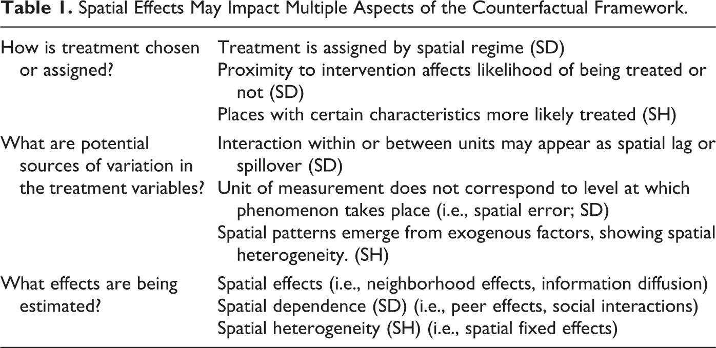
A proper spatial perspective should go beyond the uncritical implementation of spatial tools or methods. It should consider the inherently spatially and temporally dynamic, interactive nature of the populations being studied, and, as such, inform the initial design of the model. For example, is there movement within or between units that can appear as spatial spillover? Or, does the unit of measurement, if indexed by geographic area, correspond to the level at which the phenomenon takes place?
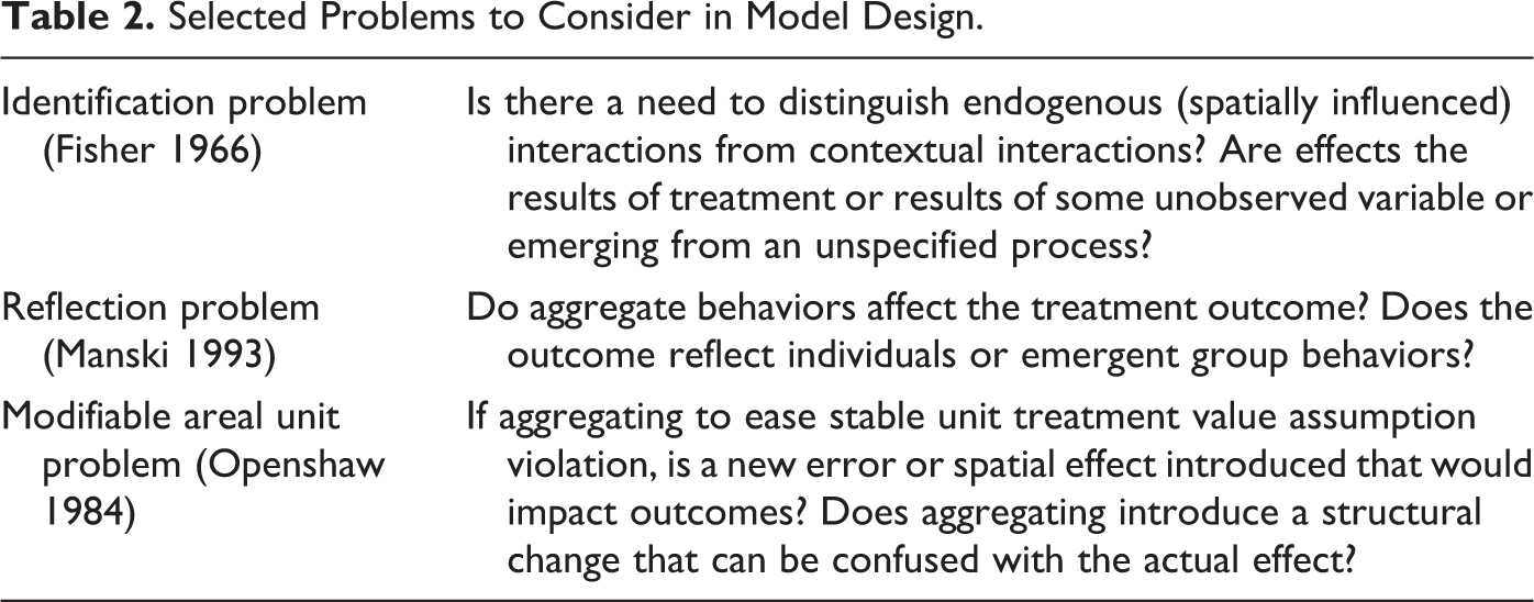
In addition, there are three distinctly spatial problems that need to be taken into account in model design: the identification problem (Fisher 1966), the reflection problem (Manski 1993), and the modifiable area unit problem (MAUP; Openshaw 1984). As summarized in Table 2, endogenous, spatially influenced interactions must be distinguished from contextual interactions, and the effect of aggregate behaviors must be accounted for. Also, by changing the spatial unit of observation (aggregation), are spatial effects introduced that could be confused with the treatment effect?
Selected Problems to Consider in Model Design.
In practice, it may be difficult to disentangle multiple and complex spatial effects from assignment and/or treatment effects, and their simultaneous relationship(s) must be specified explicitly. Detecting the presence of spatial patterns is only the beginning, serving as descriptive tool rather than being predictive or prescriptive. The nature of spatial patterns uncovered must be considered and further specified in a formal model, making the effects explicit.
Finally, there is no “one-size-fits-all” spatial specification to account for all spatial effects, and an explicit model requires specific consideration. Rather, a spatial perspective must inform the researcher when considering which specialized methods should be used to account for research design challenges.
A Spatial Perspective on Treatment Effect Evaluation
Methodological challenges posed by the identification problem, reflection problem, and MAUP impact research resign in treatment effect analysis and causal inference, all violating the SUTVA. This has led to an extensive literature that deals with techniques that incorporate quasi-experimental research designs such as differences in differences (DID), propensity score and matching, regression discontinuity, and instrumental variables (IV; Abbring and Heckman 2007; Gangl 2010; Guo and Fraser 2010; Heckman 2010; Imbens and Wooldridge 2009; Morgan and Winship 2014; Pearl 2009a; Rubin 2006; Shadish, Cook, and Campbell 2002).
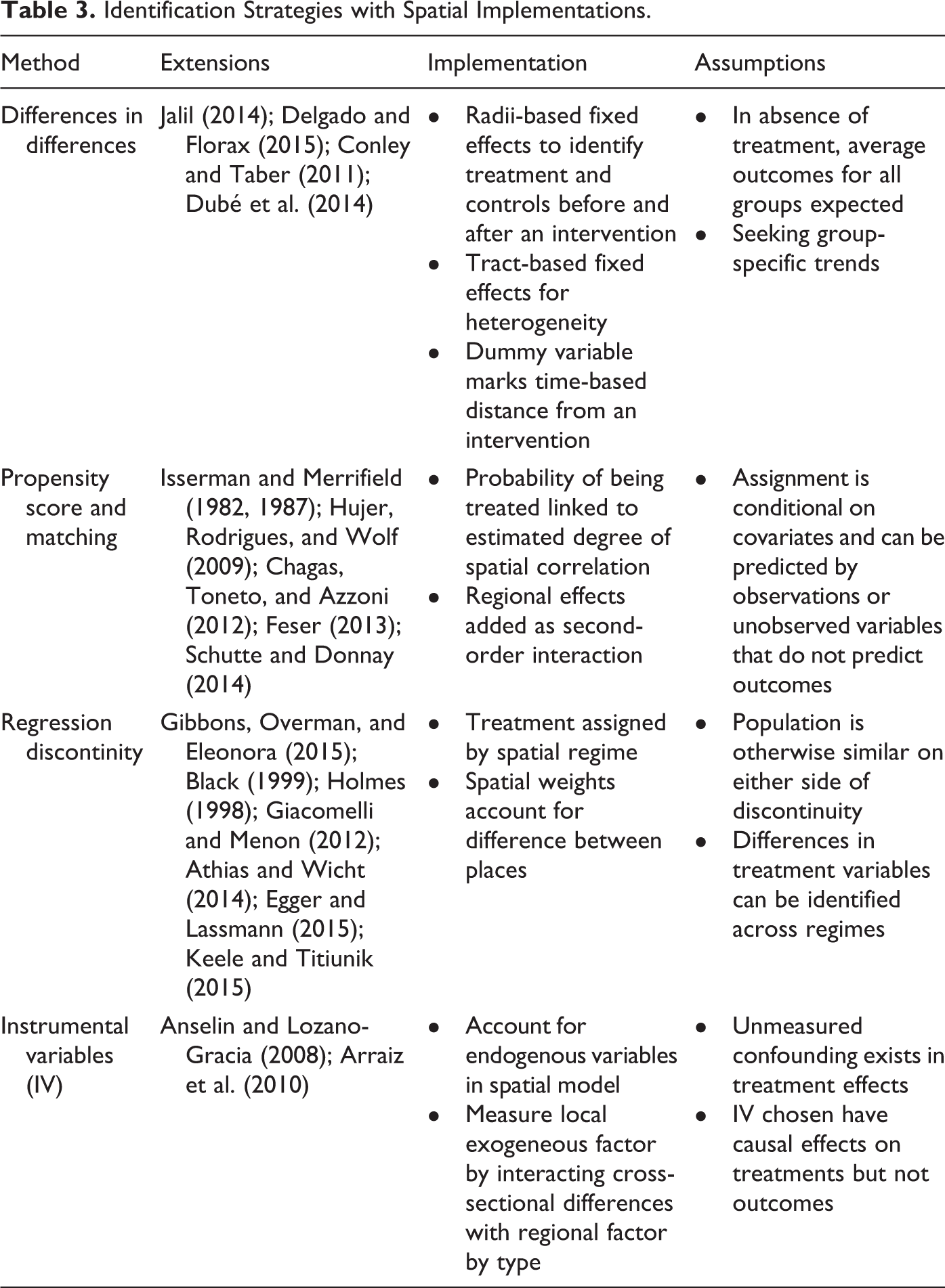
In this section, we briefly review each of these methods in turn and explore how spatial effects can be incorporated. An overview of the main issues and studies is provided in Table 3. We focus on the cross-sectional and spatial panel setting and do not cover multilevel designs. While the latter is commonly applied for this purpose, the explicit treatment of spatial effects in multilevel settings is still in its infancy.
Identification Strategies with Spatial Implementations.
Decomposition methods as an identification strategy also emerges from the program evaluation literature but within an applied economic setting. The term “counterfactual” here specifies counterfactual scenarios or experiments that attempt to define how treatments would differ based on differing hypothesized counterfactual distributions of some factor (often measured as a scalar value) impacting outcomes. Carrillo and Rothbaum (2016) provide an overview of counterfactual spatial distributions as a necessary extension in the context of decomposition economics, building on work by Fortin, Lemieux, and Firpo (2011) and others. Our discussion extends more broadly beyond the counterfactual context of decomposition strategies, focusing instead on the distillation of the research design required in counterfactual research across multiple methods.
DID
A simple DID design observes outcomes for two groups over two time periods. One group is exposed to treatment in one of the time periods, and the second group is never exposed to the treatment and serves as a control. The conventional DID design requires that in the absence of treatment, (average) outcomes for treatment and control groups will follow parallel paths over time, requiring strong underlying assumptions. Overviews of the technical issues can be found in Ashenfelter and Card (1985); Card (1990); Card and Krueger (1994); Meyer, Viscusi, and Durbin (1995); and Imbens and Wooldridge (2009).
Formally, a DID specification can be expressed as:

with the subscript i referring to location, and t referring to time.
The typical specification is as a linear model, although semiparametric techniques that allow for relaxed identification assumptions have also been pioneered (for a review, see, e.g., Abadie 2005). There are multiple challenges with a DID design, as outcomes in treatment and/or control groups may be systematically different for some reason other than the intervention studied. Additionally, ignored serial correlation may yield erroneous standard errors (Bertrand, Duflo, and Mullainathan 2004).
There have been a handful of promising, preliminary explorations of spatial effects in causal inference research using the DID approach. For example, for observations that are aggregated into groups, Conley and Taber (2011) proposed a simple model that would allow for temporal and SD and cross-sectional heteroskedasticity, depending on the group population. Heterogeneity of treatment across geographic space can be identified when investigating the differential effect of administrative borders on a policy (Jalil 2014). However, tools to detect the causation for that differentiation have not yet been fully developed. 1
Delgado and Florax (2015) introduce a spatially structured DID design by having the treatment outcomes of spatial units depend on both unit-specific applied treatment and neighboring treatments. However, this design treats the neighboring effects as unidirectional and potentially underestimates any feedback effects. A recent exploration into the development of a spatial DID estimator, using a spatial probit model, underscored the need for suitable weight matrices to account for spatial links between observations (Dubé et al. 2014).
While these approaches constitute the first steps in integrating spatial effects into a DID design, the potential effect of spatial processes affecting both structural and counterfactual aspects of the research design has not received much attention.
Propensity Score and Matching Methods
In situations where there are no observation for both pre- and posttreatment time periods, a solution has been to find “matches” or “twins” (Isserman and Merrifield 1982, 1987), that is, units that are as similar as possible in all respects other than the treatment. The treatment effect is then simply the average difference between the outcomes for the treated unit and the untreated unit. In practice, it is often very difficult to find complete matches, given the potentially high-dimensional nature of the comparison.
The method of propensity score matching, first proposed by Rosenbaum and Rubin (1983), reduces the dimensionality of the problem by so-called selection on observables. The propensity score is the probability that a unit is assigned the treatment, given a set of characteristics of the unit, say X. This can be estimated by means of a logit or probit regression. The treatment effect can then be estimated as the difference in outcomes between units with similar propensity scores, typically obtained from a second-stage regression specification (see, e.g., Baum-Snow and Ferreira [2015] for detailed examples).
Propensity score methodology may not serve for more behaviorally complex problems (Heckman and Robb 1985). Furthermore, it assumes that selection in and out of a treatment can be fully predicted by observations or unobservable variables that do not predict the outcome of interest, further limiting certain study designs (Baum-Snow and Ferreira 2015). For nonexperimental settings that consider causal inference, propensity score matching has been successful in reducing bias between treated and comparison units (e.g., see the review in Dehejia and Wahba 2002).
Spatial effects can enter into the matching/propensity score approach in two main ways. First, the matching process itself can take location and spatial interaction into account. For example, Hujer, Rodrigues, and Wolf (2009) investigated macroeconomic effects of labor market programs in West Germany using an extended matching model that accounted for spatial autocorrelation by using a specialized generalized methods of moments (GMM) estimator. Schutte and Donnay (2014) outlined a so-called matched wake analysis, which consists of a system of sliding spatiotemporal windows to select treatments and controls. However, when the resulting data cylinders overlap, they again violate the SUTVA.
A second way to account for spatial effects is the estimation of the propensity score equation. In the presence of omitted effects that show spatial structure, the resulting spatial autocorrelation will invalidate the estimates from a logit or probit model (e.g., see the extensive discussion in Fleming 2004; LeSage and Pace 2009). In addition, a spatial latent variable specification allows for the inclusion of spatial interaction among units in the form of a spatially lagged dependent variable in the model. Such an explicit spatial logit approach is outlined in a study by Chagas, Toneto, and Azzoni (2012), investigating the impact of sugarcane farming on municipalities in Brazil. This highlights the biasing effect of spatial autocorrelation on the estimates of the logit model and thus on the resulting propensity scores. A spatial probit model is an alternative specification, suggested by Franzese and Hays (2009). However, the investigation of the role of spatial effects on matching and propensity score approaches remains far from complete.
Regression Discontinuity
A regression discontinuity design (RDD) assigns a causal interpretation to a break in the data, such as a given date in a time-series context (e.g., the passing of a new regulation), or a boundary in a spatial context (within a policy zone or outside a policy zone). The latter is referred to as a spatial regime design in a spatial econometric context, as a special case of coefficient heterogeneity (Anselin 1988). It is a common specification used in the case of a so-called natural experiment, where a treatment is applied in a well-defined spatial area but not in another. Typical examples are the effects of administrative borders, with different policy regimes on each side of the border (e.g., tax rates, minimum wage laws, environmental regulations).
In the most straightforward implementation of RDD, the break in the data is represented by an indicator variable that takes the value of 1 after a treatment was applied (or in the spatial zone where the treatment was applied) and 0 elsewhere, although more complex designs are possible as well (see the reviews in Imbens and Lemieux 2008; D. S. Lee and Lemieux 2010; Angrist and Pischke 2010, among others).
Spatial regression discontinuity has been implemented with increasing frequency in evaluating polices across administrative boundaries in economic and political studies (e.g., Black 1999; Holmes 1998; Giacomelli and Menon 2012).
When the discontinuity is spatial, the consideration of potential spatial autocorrelation in addition to the SH becomes important (see, e.g., Gibbons, Overman, and Eleonora, 2015, for a discussion). A detailed overview and formalized definition of geographic RDD from a political science perspective can be found in Keele and Titiunik (2015). The authors present challenges unique to a spatial perspective by specifying geographic boundaries as regression discontinuities, thus formalizing spatial effects. Other recent applications include Athias and Wicht (2014) and Egger and Lassmann (2015).
In these settings, the proper specification of the spatial processes involved becomes critical. This aspect has only received minor attention so far. The specification of differing spatially explicit models using RDD strategies could reflect and test different conceptual hypotheses of potential sources of variation in treatment (as detailed in Table 1). By being more explicit in how the specified models conceptually and methodologically address the spatial processes impacting treatment effect variations, existing gaps in the literature could be further addressed.
IV
Finally, we briefly mention the IV approach, which is not specific to treatment effect analysis, but is employed to control for potential endogeneity in treatment assignment. Ignoring this endogeneity may lead to biased estimates of the treatment effect (for an extensive discussion, see, e.g., Heckman 1979; Angrist, Imbens, and Rubin 1996; Angrist and Pischke 2015; Baum-Snow and Ferreira 2015).
The choice of the proper instruments is often challenging in practice. The instruments should be related to the treatments or assignments but not to the outcomes. An extension to dealing with endogeneity in spatial econometric models is straightforward (e.g., Anselin and Lozano-Gracia 2008; Arraiz et al. 2010).
Empirical Illustration: The Effect of Minimum Legal Drinking Age (MLDA) on Mortality
We illustrate how spatial effects can be made explicit in a causal analysis with an expanded replication of the Angrist and Pischke (2015, 191–203) textbook example of the investigation of the effect of US states MLDA on mortality. Angrist and Pischke (2015) implement a variation on the classic DID design, which they refer to as a “multistate regression DD” model (we return to the exact model specification below). We extend this approach with an explicit consideration of potential spatial spillover effects in a spatial panel design. Our models include a spatially lagged dependent variable as well as a spatially and space-time lagged explanatory variable. In this context, the dependent variable is the outcome of the treatment, that is, mortality, whereas the explanatory variable is the treatment. A spatially lagged treatment variables thus incorporates the effect of the treatment in neighboring states, as aspatial lag of X (SLX) model (Vega and Elhorst 2015).
In what follows, we first provide a brief review of the policy background and earlier studies, followed by an outline of the different model specifications and a comparison of the empirical results.
Policy Background
After the end of the prohibition era in 1933, most US states implemented a drinking age of twenty-one. In the early 1970s, the voting age was reduced to eighteen, and, following tension over the Vietnam War, drinking age policies were changed once again. After 1971, several states reduced their drinking age to eighteen. After 1984, federal policy shifted to pressure states into increasing the drinking age (by tying it to the receipt of fiscal expenditures for infrastructure development), and by the late 1980s, drinking age had returned to twenty-one. Some states, like California, kept their drinking age at twenty-one the entire time, while others had considerable variation at multiple points (in either direction). This resulting natural experiment of policy patchworks that took place in the United States over nearly two decades proved an ideal laboratory for quasi-experimental research. Examples of earlier causal inference studies examining the effects of this policy include Du Mouchel, Williams, and Zador (1987), Shults et al. (2001), Wagenaar and Toomey (2002), Carpenter and Dobkin (2009), Norberg, Bierut, and Grucza (2009), and McCartt, Hellinga, and Kirley (2010).
In this literature, exposure to lower MLDA has been conclusively connected with increased mortality and additional negative outcomes (McCartt, Hellinga, and Kirley 2010; Shults et al. 2001; Wagenaar and Toomey 2002). Specifically, while both mortality rates for all deaths and motor vehicle accident (MVA) deaths decreased from 1970 to 1984, MVA mortality shows a distinctly different pattern, as illustrated in Figure 1. We therefore focus on the specific effect on MVA mortality.
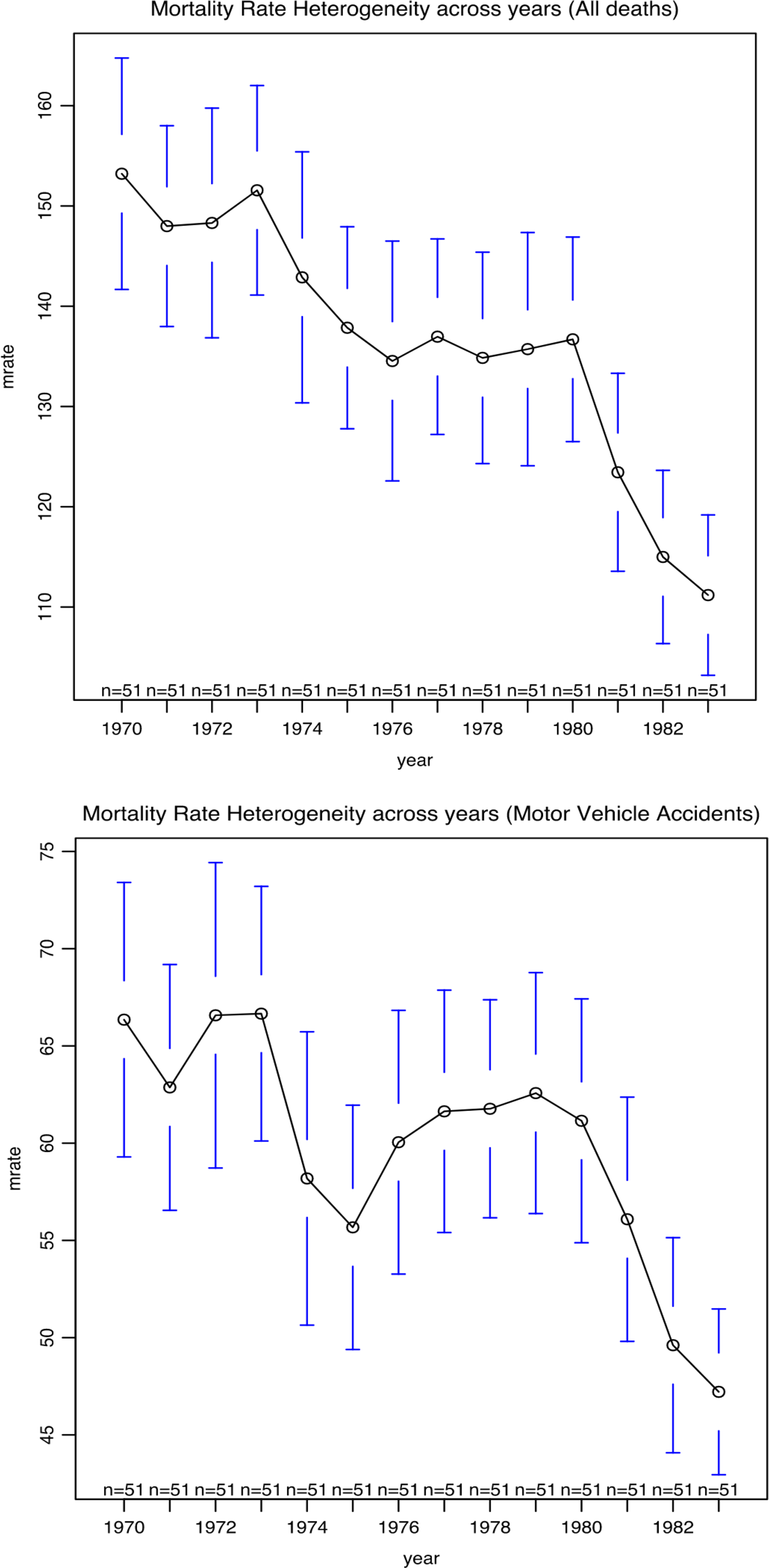
Mortality rate heterogeneity over time.
Data and Model Specifications
The basic model
The original data for state policies on alcohol purchase age can be found in Du Mouchel, Williams, and Zador (1987). In our analysis, we used the data set as reported on the website that supplements the Angrist and Pischke’s (2015) text. Mortality data for all deaths, MVAs, suicide, and internal causes were originally sourced from the US death census for the corresponding time periods, as made available by the National Center for Health Statistics. There are fifty-one “states” (the District of Columbia is included in the original data set) and fourteen time periods in the panel, ranging from 1970 to 1983. For the spatial extension, we consider only the continental states, resulting in forty-nine cross-sectional observations.
As argued in Angrist and Pischke (2015, 192–95), a standard DID design cannot be applied in this case, since there is no clear pre- and posttreatment schedule for the policy. Different states change the drinking age at different points in time. In addition, some states make the change midyear. Instead, Angrist and Pischke (2015, 194) outline a multistate regression DD model. Using their notation with some minor alterations (e.g., substituting i as the spatial subscript instead of s and shortening the year and state dummy notation), the specification takes the following form:
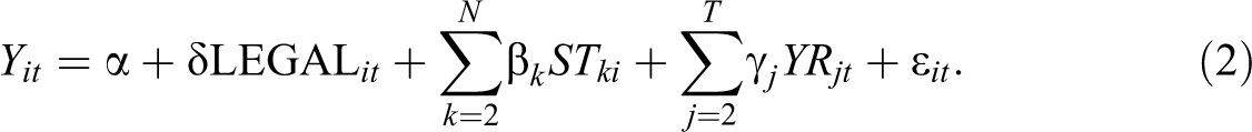
In essence, this is a spatial panel specification with N cross-sectional observations and T time periods, including state fixed effects (
The outcome variable
The fixed effects reflect the “common trend” assumption that underlies the DID logic. In order to relax this assumption somewhat, Angrist and Pischke (2015) also introduce a state-specific trend as the product of the state dummy with a time index t:

The interpretation of the inclusion of this interaction term is that the treatment effect now becomes an offset from a state-specific trend and not from a trend common to all states. The latter might mistakenly assign a causal interpretation to different time trends between states, even when no treatment effect is present.
As final adjustment, Angrist and Pischke (2015) include a control variable for beer tax.
Spatial extensions
Even though the original “multistate regression DD” is in essence a spatial panel setup, spatial effects were not considered in this context so far. As argued above, such effects enter into the counterfactual framework in a number of ways, affecting treatment assignment, potential sources of variation in treatment, and the outcomes. For example, spatial patterns may follow from intrinsic SH that is not captured by the state fixed effects. In addition, SD may affect both the outcomes (spatial spillovers in mortality impacts) and the adoption of the treatments (peer effects).
We consider five different specifications to include potential spatial effects. To simplify notation, we represent the Angrist–Pischke functional form for the fixed effects as
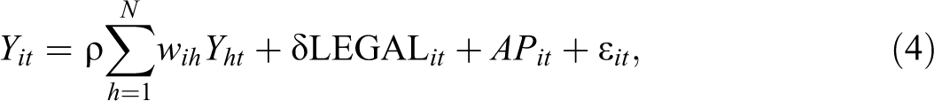
A spatially lagged dependent variable
The spatially lagged dependent variable captures the contemporaneous outcomes in the neighboring states. More specifically, the reduced form of such a model suggests that the mortality outcome in a given state is a function not only of the treatment in that state but also of the treatment in all the other states in the system, in the form of a spatial multiplier effect (Anselin 2003b).
Formally, the model is:
with
This model is estimated after first differencing (over time), which removes the state fixed effects. The so-called within estimator employs either maximum likelihood or IV to obtain consistent estimates for the spatial parameter and the regression coefficients but not for the state fixed effects (see, e.g., Elhorst 2003, 2014).
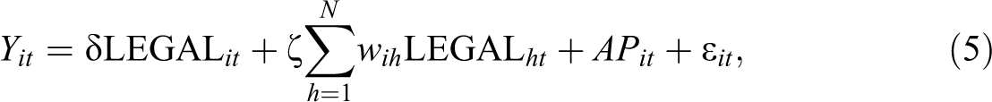
A spatially lagged treatment variable (SLX)
Whereas the spatial lagged dependent variable implies a spatial multiplier effect driven by all the cross-sectional observations, a more limited view of the spatial extent of the spillover is implemented in an SLX specification (Vega and Elhorst 2015). This includes a spatial lag of the contemporaneous treatment variable on the right-hand side of the equation.
Formally:
with again
This specification can be estimated by means of a standard panel ordinary least sqaures (OLS) approach, assuming no other forms of misspecification.
A time lagged treatment variable
The assumption of an immediate effect of the change in legal drinking age on traffic deaths may be too strong, so we also consider a specification where the treatment variable is lagged one period in time.
Formally:

In the absence of any other forms of misspecification, this model can be estimated by means of OLS. However, in order to implement the lagged treatment variable, the first year of observations (1970) is lost, and the time fixed effects need to be adjusted accordingly.
An additional space–time lagged treatment variable
Instead of a contemporaneous lagged treatment variable, a more explicit dynamic specification considers the spatial lags in the previous period in addition to the current treatment. This is a straightforward model to capture possible space–time diffusion of the treatment adoption.
Formally:

Again, the time lag results in observations for the first year being dropped, but absent other misspecifications, this model can be estimated by means of standard panel data OLS.
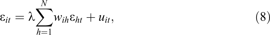
Spatial error autocorrelation
Finally, we consider the previous specification with the addition of a spatial autoregressive error term. The latter captures potential omitted factors that show a spatial pattern.
The model is the same as in equation (7) but with the addition of a spatial autoregressive error term:
with
This specification is a variant of a spatial panel fixed effects model with spatial error autocorrelation and must be estimated by means of specialized maximum likelihood or GMM methods (see, e.g., Elhorst 2003, 2014). As in the spatial lag case, consistent estimates are available for the autoregressive and regression coefficients but not for the coefficients of the fixed effects.
Results
Replication
We start by replicating the panel estimates from Angrist and Pischke (2015), corresponding to equations (2), multistate regression DD model with a common trend and (3), state-specific trend, for fifty-one states, respectively, reported in columns (1) and (2) of Table 4. The results show the estimates of the effect of minimum drinking age on MVA death rates (per 100,000) of eighteen- to twenty-year-olds. 2 As in the original study, we find a difference between the common trend and state trend estimates, with the effect dropping from 7.59 to 6.64 additional deaths attributed to the lower drinking age. However, the latter coefficient is not as significant as in the common trend model. When controlling for beer tax, reported in columns (1b) and (2b), the estimated effect increases slightly to, respectively, 8.15 (common trend) and 7.56 (state trend), both highly significant. 3 The estimates of the beer tax themselves are not significant.
Replication Results (1970–1983).
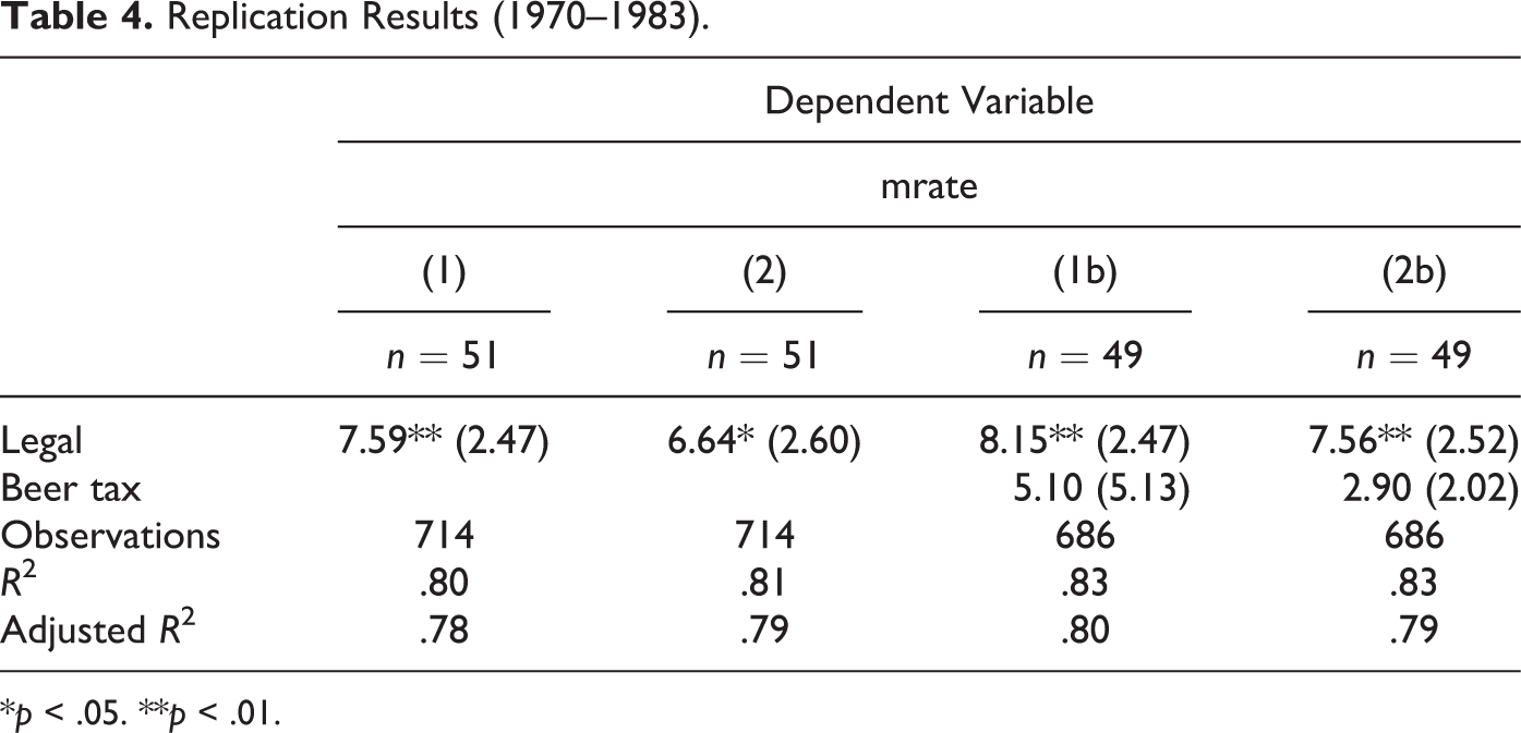
*p < .05. **p < .01.
The results are exactly the same as those reported by Angrist and Pischke (2015), except for some minor variations in the estimate of the standard error at the hundredth of a decimal point, likely due to slight differences in software implementations. 4
Diagnostics for spatial effects suggest the presence of spatial lag dependence. Specifically, the Lagrange multiplier (LM) test for spatial lag in the base model for forty-nine states was 7.76 (with
Some interesting insights can be gained from the estimates of the state fixed effects, that is, the extent to which in particular states the mortality rate is greater or lower. The state coefficients in the state-trend model showed a significant overall Moran’s I of .36 (queen contiguity). An exploratory look at the local patterns in these coefficients suggests a cluster of Western states with disproportionally high MVA mortality and a low mortality cluster in the northeast. Interestingly, California, Utah, and Colorado turn out to be spatial outliers, with lower mortality contrasted with higher values in the surrounding states. New Hampshire is a spatial outlier in the other direction. It should be noted that these results are purely suggestive, since the estimated coefficients are not actual data but estimates that incorporate randomness. The latter is of course ignored in the local spatial autocorrelation analysis.
Spatial Models
We report the effect of incorporating the various forms of spatial effects in Table 5. The first column replicates the standard specification with state trend for our cross section of forty-nine state for 1971 to 1983. 5 The second column extends the standard specification with a spatially lagged dependent variable (with coefficient ρ). The next three columns include various forms of a spatially and serially lagged treatment variable (legal), whereas the final column shows the base model with a spatially autoregressive error term (with coefficient λ).
Spatial Effect Results (Forty-nine States, 1971–1983).
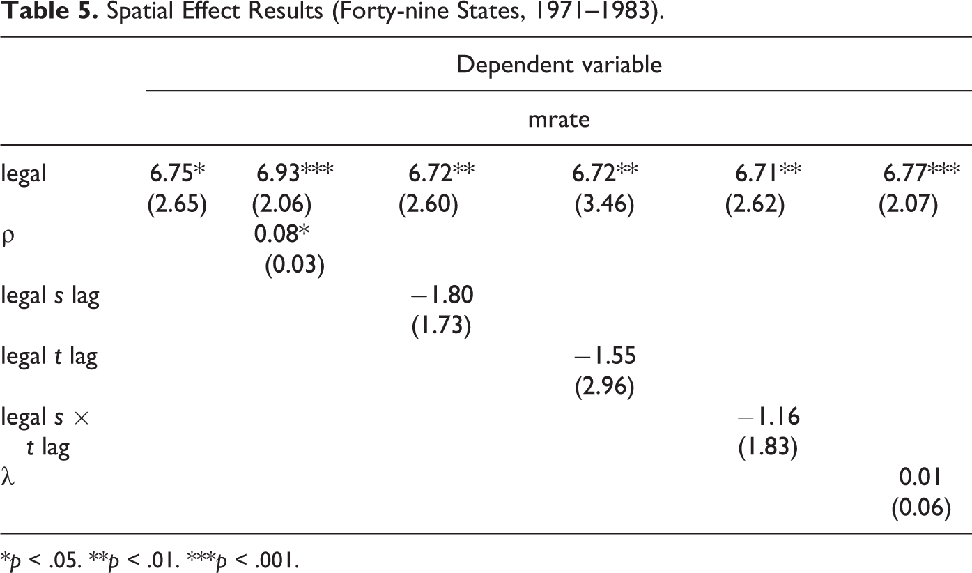
*p < .05. **p < .01. ***p < .001.
There are multiple potential sources of variation in the treatment variables, several of which can be proxied as a spatial effect. For example, the spatially indexed state variables of the classic Angrist and Pischke specification denote a case of SH, where spatial patterns emerge from state-specific exogenous factors like variations in speed limits, rural versus urban driving patterns, and physical geography manifestations. Because spatial autocorrelation still persists after this specification, we know that not all spatial effects were captured successfully. A state may also be influenced by their neighbor’s policy implementation; that is, a successful policy nearby may influence state policy makers to adopt a change (spatial multiplier effect). Thus, interaction within states may appear as a spatial lag. Similar driving patterns may further serve as a form of interaction influencing nearby states rather than assuming a sharp change drawn at the borders. States may also demand a different policy to act in competition with its neighbors. Additional hypotheses were thus specified as an interaction between states captured as a spatially lagged MVA mortality (spatial lag model), influence of nearby state policy (SLX model), impact of previous year’s policy (temporal lag model), or interaction of neighboring state’s policy in previous year (spatial and temporal lag model). By constructing multiple models reflecting different hypothesized sources of variation in the treatment variables, we further refine our interpretation of the base model.
The treatment effect of the drinking age policy variable (legal) remains significant in all spatial models (and slightly more significant than in the base model), with only minor differences between the estimates. Spatial specifications utilize the same weight matrices; however, the interpretation of spatial effect or underlying process is different in each. The spatial lag model implied a global spatial multiplier effect, whereas the SLX model implies a localized spatial effect. The largest estimate is for the spatial lag model at 6.93, which exceeds the replication estimate by a slight 0.2. This is the specification that suggests the strongest spatial multiplier effect, ranging beyond the immediate neighbors. The latter only is included in the lagged treatment variables, which are all negative, although not significant. This is an interesting contrast to the interpretation of the spatial autoregressive coefficient ρ, which, why small, is significant and suggests a positive spatial multiplier effect. More precisely, the effect of the immediate neighbors is to lessen the impact of legal driving on motor vehicle deaths, whereas the spatial multiplier suggests the opposite. Lagged treatment variables of the SLX model showed a localized and dampening effect of the treatment, whereas the spatial multiplier model demonstrated a global phenomenon of state-by-state interaction that ultimately boosted treatment
The spatial multiplier effect can be decomposed into a direct effect of 6.93 per 100,000 and an indirect effect of 0.61, for a total effect of 7.55, almost one death per 100,000 more than the aspatial estimate. Moreover, the contribution of the spatial model is to dissect this effect into a local factor and one attributable to a spillover from the policies in all neighboring states. The lack of significance of the coefficients in the SLX models suggests a global pattern of spatial spillover rather than a local one. While these spatial models do not add significant change to the estimates, they provide a clarification in understanding. Facilitating a more thoughtful interpretation of the underlying processes is critical to causal inference problems.
Conclusion
In the review of common identification strategies for counterfactual frameworks in quasi-experimental research design, we identified areas where the treatment of spatial effects is relevant. Early applications of spatial processes can be found in DID and fixed effects, regression discontinuity, IV, and matching techniques. However, the complexity and nuance of different spatial concepts underlying different processes remains to be fully implemented in a counterfactual framework. We outlined a spatially explicit counterfactual framework that formally considers how spatial effects can impact each structural component of a causal research design setting (following Heckman organizing principles) and apply those concepts using a Rubin, program evaluation–specific framework.
Spatial effects can serve as a proxy for many underlying processes in complex problems common to urban and regional policy. By specifying these in the correct way, after first effectively diagnosing the observed spatial pattern, the SUTVA of no intraunit interaction may be relaxed. To demonstrate these concepts in practice, we replicated and extended a standard policy study of measuring drinking age policy effects on mortality. Not only was the treatment effect a highly spatial phenomenon, but its distribution reflected multiple spatial processes.
Identifying the types of spatial effects presented in a problem is necessary in research design to avoid their misspecification. A suite of existing spatial diagnostics and exploratory spatial data analysis techniques can be implemented to define those spatial concepts, as reviewed in this essay and implemented in the empirical example. By extending a counterfactual analysis directly in a spatial panel econometric model, identified spatial effects (that in turn proxy for underlying processes) are formalized. Not only does this correct for potential misspecifications, but it also provides insight into the range and strength of the spillovers involved.
Methodological techniques from spatial econometrics allow for greater insight in complicated quasi-experimental problems that often challenge SUTVAs. With more place-based programs and interventions considered in urban and regional policy, greater understanding is needed to determine how such a policy impacts nearby places (for better or worse). Incorporating spatial effects into formal causal inference modeling within this natural experimental framework should lead to a deepened understanding of the treatment effect.
Footnotes
Authors’ Note
Earlier versions were presented at the Sixty-fourth Annual Meeting of the North American Regional Science Council (Vancouver, BC) and the Fifty-seventh Annual Meeting of the Western Regional Science Association (Passadena, CA).
Acknowledgments
Comments by the participants in the sessions are gratefully acknowledged, especially from the discussants Jan Rouwendal and Sandy Dall Erba. Thanks also to Julia Koschinsky, Paul Elhorst, and James LeSage for useful suggestions.
Declaration of Conflicting Interests
The author(s) declared no potential conflicts of interest with respect to the research, authorship, and/or publication of this article.
Funding
The author(s) disclosed receipt of the following financial support for the research, authorship, and/or publication of this article: This research was funded in part by Award 1R01HS021752-01A1 from the Agency for Healthcare Research and Quality (AHRQ), “Advancing spatial evaluation methods to improve healthcare efficiency and quality.”