




Abstract
We present a comprehensive agent-based model of a closed system of cities. The model includes two types of agents—employees and firms. Firms compete for workers and make decisions concerning what to produce and whether to adopt innovations. Individual employees make migration decisions. Some migrants become intrapreneurs when their employers adopt production process innovations that they propose. Some migrants become entrepreneurs when the product innovations that they propose are implemented by their employers in new subsidiary firms. These firms tend to be technological leaders. The decisions of individuals and of firms generate innovation–migration dynamics that generate a variety of city sizes. A city that is home to firms that are currently relatively attractive to migrating innovators experience moderate or fast growth. Because of particular decision patterns by individuals and firms, this growth may decline and stop, and the city may stagnate and loose workers as its relative attractiveness decreases. Cities that remain unattractive for long periods can stop growing and shrink. We model explicitly the extent to which cities attract immigrants and innovators and demonstrate that the size distribution of cities is defined by the ability of its resident firms to adopt the innovations and to let the product innovators establish technologically advanced enterprises. These decisions result in high market value of the most productive firms, of the entire industrial system the city where the firm is located, and of the entire urban system.
Keywords
Introduction
The rank–size rule for cities, often referred as Zipf’s law, suggests that the size of a city is inversely proportional to its rank. This is a remarkable and seemingly stable regularity in systems of urban regions (Gabaix and Ioannides 2004). The rule suggests a specific dynamic process that seems to govern the growth of systems of cities. Empirical evidence of a power law in a system of cities is considered as indicating one or more of several very general system mechanisms such as preferential attachment, criticality, or multiplicative processes (Gabaix 1999; Dittmar 2009; Corominas-Murtra, Hanel, and Thurner 2017). But, despite the vast empirical literature on urban power laws, there remain some controversial issues related to, for example, the absence of a universal definition of urban boundaries (Masucci et al. 2015). The vast majority of the empirical literature about the rank–size rule for cities uses population density data for administrative areas such as metropolitan areas (Eeckhout 2004) or cities (Giesen and Suedekum 2010). Rank–size estimates obtained for predefined geographical areas show great variety, even if the set of cities and the historical periods are the same (Ioannides and Overman 2003; Black and Henderson 2003). For this reason, some scholars doubt the ubiquity of power laws (Benguigui and Blumenfeld-Lieberthal 2007; Arcaute et al. 2015; Broido and Clauset 2019). It is important to emphasize that rank–size distribution shows the status of a system of cities at a specific point of time and can vary in time. These are instantaneous realizations of prolonged and at times chaotic dynamics of individual cities in the urban system (Batty 2006). We argue that the exclusive use of scaling laws obscures a rich variety of underlying life cycles and interactions among them for systems of cities.
In this article, we propose an agent-based model (ABM) by means of which we explore simultaneously two well-known stylized facts concerning cities—life cycles of individual cities and power law for groups of cities. Our model provides a novel platform for the analysis of how these phenomena are affected by the interfirm and interurban migration of the work force and by the amount and economic growth potential due to innovation adoptions by firms. Under very general conditions, our model generates entire life cycles and long tail distributions that satisfy a power law. The emergent fluctuations in the composition of firms in cities and their attractiveness to innovators, especially when maintained for long periods, lead to clearly identifiable stages of cities’ life cycles. Some cities produce full life cycles, including growth, stagnation, decline, and renewed growth. Some cities experience partial cycles only. The indeterminism of the system’s development is high, and the city size distributions for the same set of model parameters can vary significantly.
The basic building block of the model is comprised of firms located in a particular city. Firms do not migrate. Each firm is seeking to increase its profits and to grow. It can achieve this by increasing revenues and/or decreasing costs. In this article, we emphasize the first option and assume that a firm can increase revenues by implementing innovations. The latter can be process innovations resulting in modest repercussions, leaving firms in the same industrial sector. It can be radical product innovation with new products that upgrade the firm to more advanced technological sectors (Demircioglu, Audretsch, and Slaper 2019). Economic development is associated with the growth and decline of firms, which is an evolutionary, out-of-equilibrium process. It is driven by entrepreneurial actions of individuals within existing or new firms. Firms adopt technological innovations, creating new products, services, and production processes giving rise to Schumpeterian creative destruction (Schumpeter and Opie 1961). In the absence of innovative behavior, the economy will slip into a stationary equilibrium state (Kim and Mauborgne 1999). Individuals are the source of innovative ideas in our model. To be implemented, an invention should be either adopted by a firm where the inventor works in the case of process innovation or be implemented within a new, subsidiary firm in case of product innovation. Some innovative ideas are simply ignored. Workers, including innovators, take decisions about their employment and can move to a new firm (whether in the same city or in a new one). We model explicitly the extent to which cities attract immigrants at the expense of other cities. As in Gabaix (1999), the population of our system is fixed. It is a closed system. However, in contrast, we allow for interurban migration. Our model enables us to study the varied impact of the resulting innovation–migration dynamics on cities (Fujita, Krugman, and Venables 1999; Fujita and Thisse 2002; Felsenstein 2011; Kemeny 2017; Solheim and Fitjar 2018). Cities that attract migrants and/or innovators experience moderate or fast growth (Herstad and Sandven 2019). Cities that do not attract migrants or innovators may experience stagnation or even shrinkage (Lee and Rodrıguez-Pose 2013).
The rest of this article includes three sections. The second section presents a detailed description of our model. The results of model simulations are presented in the third section. In the last section, we present a discussion of the results and speculations concerning future work.
Model Description
Model’s Building Blocks
The model’s “country” is comprised of a fixed number of cities and a fixed number of workers who live in the country and work in one of the firms. The workers live in the same city where their employer firm is located. However, they are mobile and can move to another firm in the same or in a different city. Although the workers’ population is constant, the cities’ sizes change in time, as workers migrate by choosing where to live and work.
Initially, each city starts with the same number of firms. New firms are created during the model’s run, and each firm remains in its city of birth. The main characteristic of each firm is its market value that is assigned at a moment of firm’s establishment. The market value represents the quality of the products produced by the firm and the technologies applied in the production processes. As more production process innovations are adopted by the firm, its market value increases. The invention of new products and services gives rise to new firms, specialized in serving new markets, that old firms cannot serve.
Firms compete for workers, and they remain active until the last worker leaves to work elsewhere. Workers are the innovative force that determines the system’s economic development. They constantly search for better opportunities in increasingly advanced technological environment. The extant technology is driven by worker’s innovations and firm’s willingness to implement them. The model advances in time steps, and the next sections describe what happens at each step.
The Behavior of Workers
Cities are located far apart, at a distance such that it does not permit commuting. Thus, workers live in the same city where their employer firm is located. At each time step, a worker takes three decisions (Figure 1).

Workers’ decisions that are taken at each time step.
First, a worker can continue with her current job or consider moving to another firm located in the same or a different city. The probability to migrate is constant. The final migration decision is made based on the potential salary increase that creates a positive incentive to move and the future cost of leaving that acts as a deterrent factor. To estimate the benefits from moving, the worker evaluates the current and potential salaries w relative to cost of living in her current city A and a city B, the latter proportional to the logarithm of the city’s population:

where
Assuming that the cost of moving is a fraction k of the expected real salary in the new firm/city, a worker migrates if the following condition holds:

Otherwise, the worker remains at her current job. This is consistent with the classical migration model (Harris and Todaro 1970).
Workers are the bearers of innovations in the model. The emergence of innovations is a latent process. In theory, the worker in the model can compare her personal experience with the technology, production processes, and organizational culture of the employing firm and suggest an innovation. In practice, we apply a constant probability to become an innovator. The worker can propose innovation in the firm’s production processes and/or a new product. These types of innovations are very different. While process innovation increases the firm’s market value only marginally, product innovation implies a qualitative leap into the production of a new product and operation in a new market. Product innovation generates a fundamental upgrade in the firm’s business that can only be implemented by means of a subsidiary firm managed by the innovator. The nature of both types of innovations is expressed by the persistence of the innovator. If not implemented, a process innovation is soon forgotten by the worker, while a product innovation becomes part of the worker’s entrepreneurial personality. Workers who cannot implement their product innovators with the help of their current firm migrate to another firm, and this they do time and again, trying to implement their idea.
Workers become product innovators randomly with probability
The Behavior of Firms
Firms are profit maximizing entities that produce and deliver products. Each firm (f) belongs to some market (m) such as traditional manufacturing or high-tech. Markets are numbered by integer numbers that define initial market value of a newly established firm that serves this market. Initial market value of high-tech firms is higher than that of firms that produce simple manufacturing products, and we initiate these differences by drawing firm’s market at t = 0 from the values between one and ten, uniformly. In time, firms adopt innovations and increase their market value. Firms differ in terms of productivity and salary levels that they offer their workers and define their attractiveness to workers.
Revenues and wages
At any point of time t, the revenue that firm fm
realizes,

The firm’s owners receive a share of 20 percent of the revenues, while the remaining 80 percent is distributed equally among the firm’s workers as a salary. Each worker in firm f is thus paid

Firms’ behavior
At each time step, a firm takes decision whether to adopt process and/or product innovations proposed by their workers (Figure 2). The market value of a firm is the result of the cumulative number of process innovations implemented by the firm from the moment of its establishment until the present time. Firms accumulate process innovations, creating technological footprint within its market. Let firm fm
be established at t
0, and its initial market value be

Firm’s decisions that are taken at each time step.

The value of α is chosen to limit firm’s
The new firm will be technologically more advanced than its mother firm fm
. The minimal market value of the newly created firm g is the initial market value for the market m of the mother’s firm fm
. The maximal market value of a new firm g in a city A depends on the market within which the firm will end up operating. This may be the market in the city is located or it can be a global market encompassing all the cities in the system. In the first case, maximum market value of g will be
We assume that a new firm g that is a subsidiary of a firm fm
and is established at a time step t
0 reflects global market with a probability

and with probability γ from the integer numbers on

The chosen market value m
1 is multiplied by the potential growth constant c that is randomly and uniformly chosen from the interval [1, 10]. The value of

If
The maximal number of innovations that can be adopted by a firm at a given time step is set with an equal probability as 1, 2, or 3. They are adopted with respect to the number of product innovators in the city and city’s size. Each innovation is reflecting the city’s or the system’s level separately. As mentioned above, the inventor of a product waits for the adoption of her innovation for up to ten time steps and, if it is not adopted, migrates to another firm.
The goal of our model is to study the effects of innovations and migration on the economic development of an urban system. There are three levels of aggregation in the model—individual workers, firms, and cities. Workers and firms make decisions, while cities are passive entities that change as a result of these decisions. Firms make decisions concerning what to produce. At times they hire additional workers who introduce innovative ideas. Firms adopt or reject these ideas. Individuals make decisions whether to migrate to new firms and cities as an alternative to working for existing firms and whether to become intrapreneurs in case their new employer adopts their ideas or entrepreneurs in case their ideas are rejected. Thus, the development in the model is driven by entrepreneurial actions that introduce technological innovations, creating new products, services, and production processes. The decision rules governing the agents’ behavior create an interplay between self-enforcing processes of emergence/endogenous growth and cost of living as a function of the city size.
Results
In this section, we present simulation results that illustrate the basic properties of the emerging system of cities. We highlight the collective dynamics of firms in cities at different stages of their dynamics and present the emerging cities’ size distribution.
In all scenarios, we start with the same initial conditions: at
The Basic Scenario
In the basic scenario, we assume that the market value of a new firm is influenced by the local market only, that is,
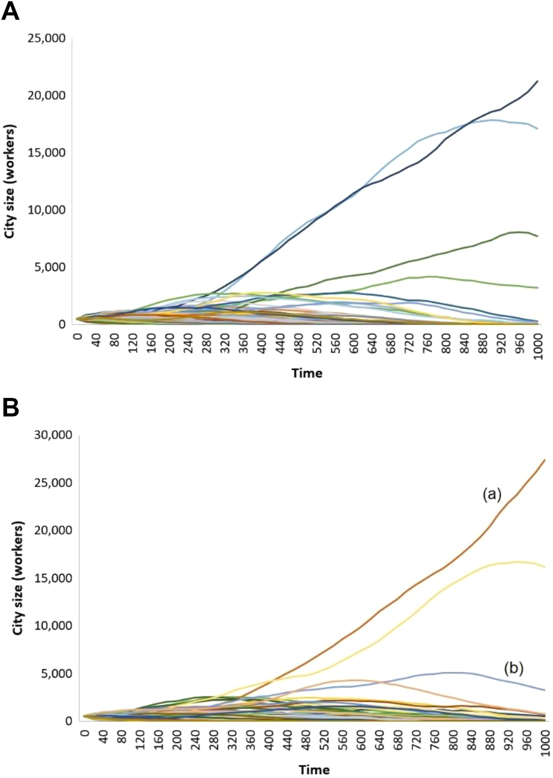
Typical dynamics of the system: Two coexisting large cities (A) and one large city (B).
Random differences in initial market value of firms are sufficient to create divergence in cities’ dynamics. Some cities are growing during the entire history of the model runs, some decline and disappear while some exhibit waves of growth/decline. The urban development path is intimately related to the accumulation over time of innovations in the firms and in the city, the wealth created, and the attraction exerted by the city for potential migrants. Every repetition of the model run generates different dynamics, as two steadily growing and competing cities, one of them winning and the other starting to stagnate at the last stage (Figure 3A) compared to constantly dominating city (Figure 3B). In both scenarios, two middle-size cities struggle to maintain their share of the population, while all other cities, including those growing in the beginning, steadily shrink later.
Most innovators migrate to the large and growing cities and those who have an idea for new products establish new firms. Large firms that are able to adopt production innovations and supply work force to the new firms enforce this positive feedback: on average, the market value of new firms is higher and higher, allowing for higher salaries and increasing attractiveness of the firms located there for other innovators. The smaller the city, the lower are the chances that its firms will attract migrants and innovators.
The fate of the new firm f depends strongly on the firm’s initial market m and the corresponding market value

Dynamics of the firms’ emergence in the (A) largest and constantly growing and stable and (B) slightly declining cities (cities A and B from Figure 3B, see small insert) and distribution of the firms’ market values in these cities at t = 1,000.
We now consider the urban system as a whole by means of the rank–size distribution of the cities. To construct this distribution, we consider cities with more than twenty workers. Figure 5 presents rank–size distributions for two runs of the basic scenario presented in Figure 3. The rank–size distributions in Figure 5 are typical of the highly concentrated urban system. More than 95 percent of the total population lives in four large cities, while the rest is distributed among many smaller towns. The distributions have a typical long tail. Several positive feedbacks in the system cause essential stochastic variation of the power law regression coefficient (Figure 6). However, all qualitative characteristics of the emergent system—the variety of individual cities dynamics, the birth and decline of the firms and distribution of their birth time at t = 1,000, and power law for the cities, with population is above the twenty-worker threshold, are preserved. Note that the regression coefficient in Figure 6 varies between −3.53 and −2.62 with the average value close to −3, which is much lower than Zipf’s coefficient of −1.

Rank–size distribution of the cities size at t = 1,000 for two runs presented in Figure 3. (A) The case of two largest cities, nine cities with more than twenty workers. (B) The case of one largest city, nineteen cities with more than twenty workers.
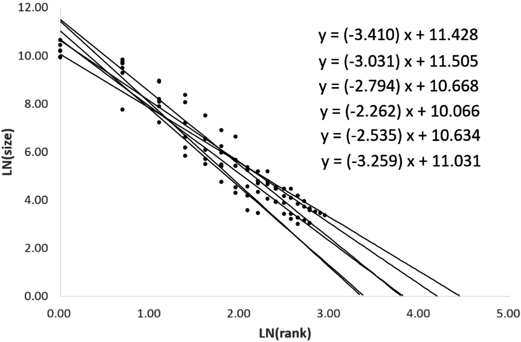
Power law dependencies for six repetitions of the basic scenario based on cities with more than twenty workers.
Effect of the Model Parameters
The level of model abstraction is high, and thus, we are interested in the qualitative effects only. Most of the parameters influence system dynamics quantitatively, resembling the results observed in the basic scenario. We studied the model’s sensitivity with various versions of the model. In particular, we were concerned with the impact of changes in the values of the probability of the local market influence γ, of the rate of product innovation λ1 and of the rate of process innovation λ2 on the innovative behavior of workers and firms.
Model sensitivity to the process innovation ratio λ2 is limited, since the firm’s reaction to accumulated process innovations is limited. Setting λ2 to different values, including zero, does not modify system’s dynamics. The other two parameters, product innovation rate λ1 and the probability of the local market influence γ, proved to be qualitatively influential. In particular, the model dynamics are qualitatively different for the case of λ1 = 0 versus λ1 > 0. Model dynamics for the different positive values of λ1 are similar to those presented in Figures 5 and 6, and the power law coefficient vary between −2.5 and −3.5. However, the existence of product innovations is crucial, and when they are canceled (λ1 = 0), the dynamics of the urban system is slow and linear (Figure 7).
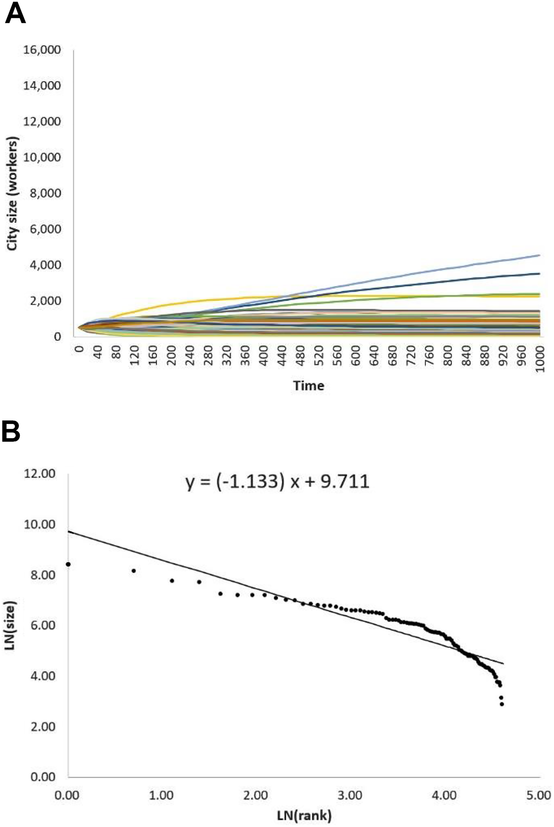
The general view of the city dynamics (A) and rank–size distribution of cities with more than twenty workers (B) in case of zero product innovation rate.
The rest of the parameters are the same as in Figures 5 and 6. At t = 1,000, the population of the biggest city is less than 5,000 workers, compared with 25,000–30,000 in the basic model (Figure 3). The rank–size distribution (Figure 7B) is also qualitatively different from that obtained in basic model (Figures 5 and 6). First, the distribution has a clear “corner.” That is, the rank–size distribution of relatively big cities is quantitatively different from those that are small. The slow pace of development of the urban system clearly manifests that product innovation is a critical link in the dynamics of the model system. The mere existence of product innovations is the engine that sparks dynamism on the urban system.
Quantitatively, the development and the shape of the urban system are intrinsically connected with the relation between product innovations and the intellectual and physical infrastructures that make such innovations possible. The local market influence defined in the basic model (γ = 0) implies a strict Marshallian interpretation of technological innovations: Only in places where people are ready to accept new ideas, the mindset is mature enough to cope with them, and the necessary means are available, product innovations can thrive. The model implements this idea by allowing new firms created in the city to be assigned a market value from great range of numbers, giving rise to a virtuous development cycle that is restricted to local firms only. Since such virtuous cycle only seldom arises, there are few cities that experience it, while most cities remain in a technologically stagnating state. This type of development created urban systems as these displayed in Figure 5, with most of the population concentrated in one or two cities.
However, relaxing the condition and assigning γ > 0 the system’s outcome changes. The assumed condition means that there is a nonzero chance that a new firm created in the city will adopt global standards, drawing its market value from the full range of values existing in the world. In other words, new firms have a chance to develop new technologies that stem from previous advances implemented anywhere worldwide. Therefore, all cities have better chance to compete for workers in the urban system. And yet although there are very large cities, the pattern of one or two largely populated cities much bigger than other cities disappears. As γ increases (allowing a more globally integrated market), the urban system becomes less heterogeneous, the population is more distributed, and the log-log regression tend to be less steep, as shown in Figure 8.

General view of the city dynamics (A, C) and rank–size distribution of cities with more than twenty workers (B, D) in case of γ = 0.1 (upper row) and γ = 0.9 (lower row).
An additional characteristic of the urban system that changes with the local market value diminution is the life cycle of some cities. In the basic scenario, the biggest city grows steadily. The other cities do not grow much and experience a single long cycle of moderate growth followed by a steady decline (Figure 3). The life cycles of cities in Figure 8 are much more erratic and complex, since the ability of any city to attract migration depends on the birth of local advanced technological firms, and this can happen everywhere and anywhere. For the same reason, the competition for workers among cities becomes more chaotic as the value of γ increases.
Figure 9 provides a summary of the two aggregate characteristics of the urban system as dependent on γ: they include the slope of the log-log regression line and the number of large cities that comprise 95 percent of the total population. As the value of γ increases, the number of the large cities increases, while the rank–size distribution becomes flatter.
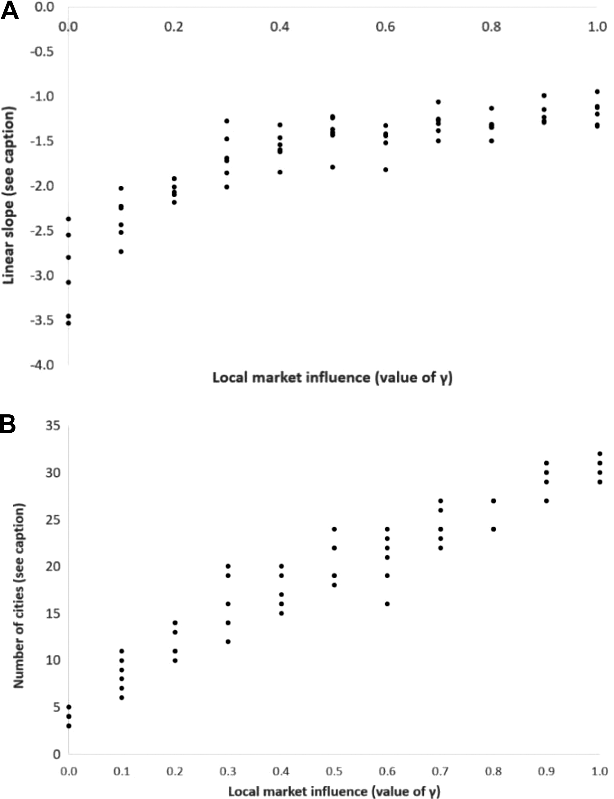
The slope of the power law of cities with more than twenty workers (A) and the number of cities that comprise 95 percent of the workers’ population (B) as a function of γ.
As is evident from this figure, parameters of the model log-log regressions depend on γ, and their range is essentially wider than observed empirically. For the real urban systems, the coefficient of regression of the city size log on city’s rank log varies, typically, between −0.8 and −1.2 (Gabaix and Ioannides 2004). In our model, the values in this range are obtained for the values of γ close to γ = 0.5. We consider this fact as an argument in favor of the mixed influence of the technological state of city and of the entire system on the innovators’ inventions. Some of them are limited to the city market, while some follow the system-wide tendencies.
Conclusions and Future Research
The motivation for the model described and analyzed in this article are the unanswered questions concerning the simultaneous existence of life cycles for individual cities and power law for their assemblage. We consider a system of cities that are comprised of firms that employ potential innovators who are able to migrate between firms and cities. In contrast to the traditional, equilibrium-oriented framework, we propose an ABM that describes workers’ migration behavior and firms’ adoption of innovations proposed by the workers. We do not presume equilibrium. The system is driven by the innovations brought in by individual inventors—workers. Innovations strengthen positive feedbacks—more innovations → more attractive firms → better city’s economy → more migrants → more innovations that enforce constant changes in the cities’ composition of firms and firms’ working force and result in persistent emergent and disequilibrium dynamics. The analysis of the model suggests that innovation–migration dynamics can explain a wide range of city dynamics including whole life cycles of cities and the size distribution that follows a power law for the cities that comprise the vast majority of country’s population.
The current version of the model has some clear limitations. Our system of cities is isolated from the outer world, and the number of workers remains constant. Innovations and migrations are the only driving forces of our “closed economy.” We did not consider, for example, policies intended to overcome divergence among cities in terms of size and economics performance. Such policies are almost ubiquitous, especially in Europe, to overcome the continuous decline of medium size cities. In contrast to our simulations, real-world size distribution of cities is influenced by such policies (see Iammarino, Rodriguez-Pose, and Storper 2019).
We are currently expanding the scope of the model in order to relax the assumed “closed economy” environment by opening it to interactions with the outer world for resolving the gap between the parameters of the model and real-world urban systems. We are also studying the impact of alternate policies to promote convergence.
Footnotes
Acknowledgments
Dani Broitman and Daniel Czamanski would like to thank the partial support of their research by the Israel Science Foundation, Grant Number 319/17.
Declaration of Conflicting Interests
The author(s) declared no potential conflicts of interest with respect to the research, authorship, and/or publication of this article.
Funding
The author(s) disclosed receipt of the following financial support for the research, authorship, and/or publication of this article: This study was funded by Israel Science Foundation, Grant Number 319/17.
