Does Tolling Per Kilometre Compensate for the External Costs of Trucks? A Geographical Approach for Belgium

Abstract

Using detailed Global Navigation Satellite System tracing data emitted by all trucks having a gross vehicle weight of over 3.5 tons in Belgium, this paper assesses the efficiency of the current Belgian distance tax system by analyzing its spatial coverage and the matching of the distance taxes with the external costs, globally and locally. Specifically, three research questions are addressed. First, how well do the present charge rates match with external costs? Second, the operationalization of the system requires a good spatial coverage of truck movements. Does the present system guarantee an almost universal coverage? Third, do the distance charges match the external costs? We find that if the distance tax scheme differentiates regionally, it still misses large variations in noise costs. The current tracing infrastructure also captures only part of the truck operations on the territory. If distance tolls for trucks remain the backbone of the taxation of truck operations, it then needs further refinement in time and space if one wants it to be the major tool to correct for the external costs.

Keywords

truck toll external costs transportation

Introduction

In the last decades, the European Union has unified the taxation of Heavy Goods Vehicles, also called HGV (Shepherd 2008). The Union has indeed since long promoted the implementation of a unique distance-based toll system, and approved in 1999 a new road charging directive. The main idea was to charge trucks according to different parameters under the principle of ‘user-pays’ (Gomez and Vassallo 2020; Shepherd 2008). It firstly led to the implementation of the Euro-Vignettes, a fare under the shape of a tax stickers that vehicles over 3.5 tonnes must pay to travel on the road network in European countries. These vignettes are valid during a given period of time (defined by the driver), whatever the kilometres driven by the HGV in the country. Secondly, Europe proposed to replace this time-based fare by the first distance-based tolls.

It appears that distance-based tolls are more fair than vignettes (time-based) and diesel fuel taxes to make users pay the real user costs (European Parliement 2018). Diesel taxes suffer from international tax competition. Indeed, in international trips, trucks fuel up their large tanks in the country where fuel is cheaper. The result was a race to the bottom where trucks did pay a low charge for their trip and paid it in the country with the lowest diesel taxes (see e.g. Mandell and Proost 2016; Calthrop et al. 2007). When the tracking and tolling technology became more accessible for tracking the movements of the trucks, several European countries such as, Slovakia (2004), Austria (2004), Germany (2005), Switzerland (in 2011), Poland (2011) and Belgium (2016) introduced a Vehicle Miles Travelled tax (VMT-Tax or kilometer-tax). Hence, while diesel taxes could still be avoided by “tank tourism”, distance taxes cannot be avoided. The reform of truck taxation is a well-known research challenge of regional science (see Lindsey, 2010 for the US) and has several effects. Kleist and Doll (2005) shows that increasing the value of the toll reduces the empty truck travel, but also increases the impact of trucks on the secondary not-tolled network. This impact is probably compensated by the public investment of the toll revenues that lead to an increase of employment and better infrastructure (Doll and Schaffer 2007).

However, it is hard to estimate the impact of distance taxes on the usage of heavy vehicles. Logistic companies have a strong importance in our economy, and are often considered as one of the pillars. Without them, most of the goods cannot be delivered, and the offer cannot reach the demand. To handle a big change, these companies often recreate themselves, adapt and start operate differently (Gomez and Vassallo 2020). However, it is important to note that Broaddus and Gertz (2008) show that distance tolls have not strongly impacted the sector.

A major advantage of the distance taxes is that they can be modulated in function of the external costs. As these taxes cannot be avoided, they carry the risk of tax exporting: countries with a lot of transit trucks may charge more than the external costs and infrastructure costs in order to extract revenues from transit traffic. The European Union has therefore imposed restrictions to the use of distance taxes: they cannot exceed the infrastructure costs and need to be related to the total external costs. However, implementing external costs within a toll system is challenging. External costs are not easy to estimate and are often a function of the volume of traffic on a road. This would lead us into traffic modelling where trucks optimize their routing.

Depending on the focus of the research, literature presents different types of method. With simple static model, external costs have been consider in addition to marginal costs when deriving optimal pricing policies (Verhoef 2000). Some model see external costs as a simple fixed cost per kilometer (amongst others Bickel et al. (1997), Tinch (1995), Grant-Muller et al. (2001), Eyre et al. (1997), or Hickman et al. (1999)), while other include more complex calculation such as emission and fuel consumption (Bates et al. 1991, Pfaffenbichler and Shepherd 2003, Shefer 1994). Although the approaches used are different, the general idea remains the same: to optimize the welfare to society using some monetary evaluation or cost–benefit analysis (Shepherd 2008). However, the usage of more complex models does not always tend to be more consistent with optimal policies that aim to reduce external costs while maximizing overall welfare (Shepherd 2008). This is why the approach chosen in this paper is based on the simple static model. However, instead of being focused on specific aspects such as the effect on traffic flows and modal shift, or on the optimal use of the revenues, this paper has a different point of view and methodology: it does not use any traffic model but starts from the observed trajectories of trucks revealed by the tracing data (GNSS data). For these trajectories, we compute the external costs given by simple fixed costs per kilometer (Shepherd 2008), and compare them with the toll revenues. Doing so allow us to address several research questions. First, the operationalization of the tolling system requires a good spatial coverage of truck movements. Does the present system guarantee a universal coverage? Second, do the distance charges match the external costs? Are there systematic imbalances in space, time or by type of trucks? In other words, we here aim at providing a critical view on the current tolling system: does it reach its objectives, or can it be enhanced spatially and economically?

The paper is organized as follows. In the first Section, the paper briefly presents the Belgian situation (the study area as well as the tax system for heavy vehicles, and the data used), before it describes the itineraries of trucks we reconstructed in a second Section. The following Section explains and computes the external costs before the paper maps and confronts taxes to external costs for standardized trips, globally and and spatially. This fourth Section questions the existence of trucks evading the charges by opting for non-charged substitute itineraries but it also puts forward other spatial mismatches between revenues and costs. The final Section concludes.

Study Area

The Geography of Belgium

Belgium (Figure 1) is a small and densely populated country (11.6 millions inhabitants on 33 000 sq km), located at the crossroad of major European transportation corridors. The Belgian urban network is denser in the northern part of the country, and hence inter-city distances are smaller (see e.g. Vandenbulcke et al. 2009). Most cities have sprawled into their countryside giving the impression of one Belgian urban continuum (see e.g. Tannier and Thomas 2013; Van Hecke and Vandertraeten 2019). Industrial and logistic activities tend nowadays to leave city centers and to be located at the outskirts of the urban agglomerations, often in dedicated “industrial zonings” close to major transportation axes (see e.g. Mérenne-Schoumaker et al. 2015). The territory has one of the most dense road networks in the world and counts over 150,000 km of roads among which 1763 are motorways and many others are very small streets. Only 6459 km of the Belgian roads are tolled for trucks.

Figure 1.

Map of Belgium – highways correspond to all roads with 2 × 2 lanes separated by a central berm.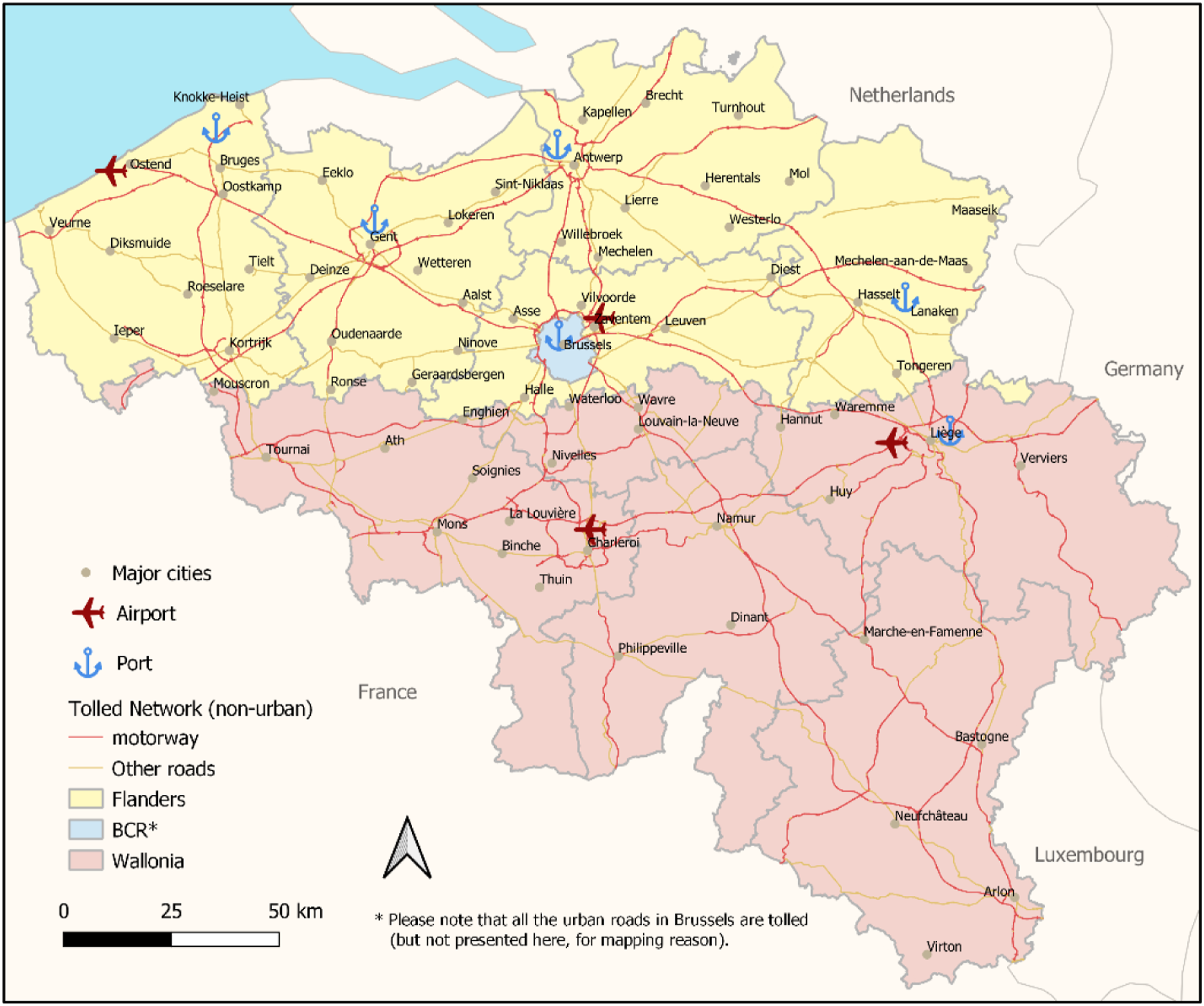

For further understanding of our results, it is important to remind that Belgium is a federal country divided into three Regions (Flemish Region (Flanders), Walloon Region (Wallonia), and the Brussels Capital Region here noted BCR). Fuel and annual truck taxes are federal, but ‘road infrastructure’ is a regional competence (see de Borger and Proost 2017). Hence the three Regions can implement their own distance tax but they have to agree on a common charging system and have also to comply with EU regulations.

The Belgian Tolling System

Since 1 April 2016, Belgium has implemented a Kilometer Charge System (KCS) that aims at internalizing the external costs of heavy-goods vehicles having a gross vehicle weight of over 3.5 tons (here called ‘trucks’): it considers the number of kilometers traveled on tolled roads (only some well-defined roads are tolled) and is modulated by the gross combination weight (tonnage) of the truck (hereafter noted GCW ) and by its emission class ( Eurovalue ) which is fixed by international directives.

To obtain the distance travelled by a truck, Belgium opted for a GNSS system via on-board units (OBU). This OBU is mandatory for all trucks circulating in Belgium, and should always be turned-on, on tolled as well as on not tolled roads. To control that aspect static and mobile cameras are used in the territory to verify that the trucks are correctly tolling (among others: OBU turn-on, no usage of a spoofing device, having a correct billing address). When the truck is standing still, it falls on “sleep mode”, and it wakes up whenever it senses motion. In practice, an OBU sends GNSS coordinates every 30 s to the back-office where they will be map-matched on the tolled network to compute the tolled distance. The tolled distance is then modulated by the characteristics of the truck (the GCW and the eurovalue). GCW is a continuous variable but for the sake of the KCS it is expressed in 3 categories (3.5 – 12 T, 12–32 T and >32 T). No toll is levied in Belgium on vehicles with a GCW smaller than 3.5 tons. Eurovalue varies from I to VI, depending on the date of the first registration of the truck and by its engine emission output in g/kWh. Class I corresponds to older trucks with very loose CO, HC, NO_x, and PM norms, while class VI corresponds to more recent trucks with strict norms in terms of pollutants. Trucks older than 1993 are put into Class 0. In case of missing values, the data provider (Viapass) manually affects an Eurovalue (see https://www.viapass.be/wp-content/uploads/2018/09/emissienormen-FR.pdf).

Table 1 gives an overview of the applied €/km toll; it shows that in Brussels (BCR), the toll is 60% higher for large trucks (>32 T). The GCW differentiation is more important: in the Flemish and Walloon Regions, large trucks (>32 T) pay 73% more per km than small ones (3.5 -12 T). Also, the Eurovalue is quite discriminating, as the dirtiest trucks pay 56% more.

Table 1.

KCS Expressed in € per Kilometre, by Region, GCW and Eurovalue in 2016.

GCW Eurovalue	Flemish Region, Walloon Region (and Motorways of BCR)			Brussels Capital Region (at the Exception of Motorways)
GCW Eurovalue	3.5 – 12 T	12-32 T	> 32 T	3.5 – 12 T	12-32 T	>32 T
0	0.146	0.196	0.200	0.188	0.263	0.292
I	0.146	0.196	0.200	0.188	0.263	0.292
II	0.146	0.196	0.200	0.188	0.263	0.292
III	0.126	0.176	0.180	0.163	0.238	0.267
IV	0.095	0.145	0.149	0.132	0.207	0.236
V	0.074	0.145	0.128	0.109	0.184	0.213
VI	0.074	0.145	0.128	0.099	0.174	0.203

NB For further information about tariffs: www.viapass.be

Taxes on Trucks in Belgium

The use of trucks in Belgium is taxed via fuel excises and distance taxes (KCS).

Fuel excises are fixed at the federal level, but many international trucks fuel up in neighbouring countries, where fuel is cheaper (Santos 2017). This is for example the case of Luxemburg where excises on diesel are much lower. The result is that without distance taxes, international trucks would use the Belgian road infrastructure for free, without paying for the wear and tear, nor for the other external costs. Combined with the replacement of the Eurovignette, this was one of the major reasons to introduce a KCS on trucks in Belgium (see Mayeres and Proost 2004).

Distance taxes face two European constraints aiming at preventing discrimination against foreign trucks in a European market objective. The first constraint is that the total revenue of the distance charges on trucks cannot exceed the total infrastructure costs attributed to trucks. An upper limit on the total tax revenue is indeed needed because some components of the external costs are subjective (e.g., “monetary value of our unique ecosystem”) and could be misused by small countries for tax exporting purposes. The second constraint is that the distance tax has to be a function of the magnitude of the external costs. The latter include wear and tear of infrastructure, air pollution, climate damage, noise, accidents and congestion. The distance tax is thus required by EU law to be proportional to external costs per vehicle km, with an upper limit of the average infrastructure cost per vehicle km. The possible differentiation of distance charges in function of external costs is determined by European regulations on trucks: the environmental categorization and the weight of the trucks. Recommended values are regularly updated and provided in a handbook on the estimation of external costs (European Commission 2019). As European countries aiming to develop their tolling systems are constrained by the external costs defined by the European Commission, we have decided to follow the criteria and values proposed by the Commission. We are confident that this choice offers a better fit of our contribution within the European context. However, readers have to keep in mind that numerous types of external cost estimates exist. Table 2 compares the parameters driving the external costs and those used to determine the distance charges for trucks. Empty cells mean no differentiation. We see that (1) distance taxes for heavy vehicles are differentiated by Region, GCW (axle weight) and Eurovalue class, and (2) the level of external costs is determined by many more parameters than those used for the differentiation of distance charges. There is only one perfect match: that between fuel excise (proportional to the quantity of CO₂ emitted) and external climate damage. Climate will hence not be considered in the following tables: fuel excises and climate damage match via fuel consumption.

Table 2.

Parameters Driving External Costs and Those Associated to Distance Charges.

External Cost	Parameters Driving External Costs			Parameters Associated to Distance Charges
External Cost	Time	Location	Vehicle	Time	Location	Vehicle
Climate	n.a.	n.a.	Fuel consumption	n.a.	n.a.	Fuel excises
Congestion	Traffic intensity	Traffic intensity + Type of road	n.a.	n.a.	Region	n.a.
Air pollution	Wind/season	Urban/rural	Eurovalue	n.a.	Region	Eurovalue
Accidents	n.a.	Type of road	n.a.	n.a.	Region	n.a.
Noise	Day/night	Urban/rural	n.a.	n.a.	Region	n.a.
Wear and tear infrastructure	n.a.	Type of road	GCW	n.a.	Region	GCW

We conclude that distance taxes are, at most, a rough average of the external costs of truck use. The current structure of distance taxes uses other parameters than the drivers of external costs except for climate that is covered via the excise taxes on fuel. This brings us to answer the first research question: the current structure of truck distance taxes does not match well with the structure of the external costs. To know how important this mismatch is, we need to estimate the relative importance of the different external costs. The estimation of the external costs will be discussed in detail in the Methodological Section.

Data

Data Description and Cleaning

The database consists of all the GNSS positions of all trucks circulating in Belgium during 1 week of November, from Monday to Sunday, and collected via the OBU, whether they were on tolled roads or not. Each GNSS point emitted by an OBU consists in the truck anonymized ID (under the “privacy by design” approach, this ID is randomly changed every day at 02:00 a.m.), the coordinates of the GNSS point, the time of the emission, the instant velocity and the direction of the truck (computed from the GNSS chip within the OBU), the country of registration of the truck, its Eurovalue and GCW.

After testing the five working days (number of trucks, amount of GNSS pings emitted, gaps within trips, or external factors like winter weather condition or strikes), only the trips made on the Tuesday 15th of November 2016 have been considered as representative and used to construct a sample of truck itineraries. Starting with 134,393 IDs for that day (from 02:00 a.m. on day1 to 01:59 a.m. on day 2), we ended up with only 91,199 trucks. It is important to clarify which trucks have not been considered in this paper: (1) trucks emitting less than 10 GNSS points (1997 trucks), and (2) all the trucks cleaned under the process developed by Finance et al., 2019 (41 197). The purpose of this last process is to remove the trucks having ‘gaps’ into their sequence of GNSS pings; these are considered as noise that would introduce biases.

Computing the toll and externality costs for each truck requires to evaluate the total distance covered by the truck, and to know if the route taken is tolled or not. The estimation of the cost is based on the next four steps.

First, the spatial road network (SIG) of the tolled roads is constructed based on the Open Street Map data and on the information provided by Viapass. Once all tolled roads are selected and cleaned to match with the official Belgian road network (Viapass), a buffer of 10 m is computed around each road segment.

Second, a grid made of 1 km² squared cell is applied on Belgium. To make the system reproducible, the grid used in this paper is the one developed by Eurostat and presented in the Methodological Section.

Third, GNSS points are map-matched with the buffer shapefile and all the information are collected (ID of the road, type of road, Region to which the road belongs), as well as the ID of the cell.

Fourth, by considering trucks individually, the Euclidean distance is computed between each successive pair of GNSS points, and the value of the toll/externality costs are computed based on the distance and the attributes collected for each GNSS points. It is important to precise that the externality costs are computed only when the GNSS points are located on the tolled road network. This allows to compare the two values.

National and International Trajectories

Trucks are registered in 48 different countries and we know that the country of registration impacts route and stop patterns, even if nowadays it is quite difficult to really link the country of registration with local market due to the strong interconnection of the European countries (Adam et al. 2021). Hence, trucks are here categorized in two groups: if all GNSS points are emitted in Belgium, the truck is considered as driving exclusively in Belgium and labelled intraBe truck, while at the opposite, if at least one GNSS point is emitted out of the Belgian territory, this truck is classified as “international” and noted interBe truck. We observe that 47% of the trucks in circulation are interBe trucks (Table 3). These interBe trucks are mostly heavy trucks (94%), while only 53% of the intraBe trucks are heavy ones. In the same vein, large Eurovalues (V and VI) represent 52% of the intraBe trucks and 84% of the interBe trucks: international (interBe) trucks are cleaner and heavier.

Table 3.

Number of Trucks (ID) and GNSS Pings by Category on 15 November 2016.

	intraBe	interBe
Number of trucks	48,173	43,026
By GCW
3.5–12 tons	10,202	777
12–32 tons	12,422	1484
>32 tons	25,549	40,765
By Eurovalue
0	2688	837
I	782	45
II	3235	208
III	9125	1815
IV	6720	1804
V	16,845	17,417
VI	8,193	18,599
Number of GNSS pings
emitted on tolled roads	8,238,632	10,045,371
emitted on non-tolled roads	10,219,688	2,950,580

Trucks moving exclusively on the Belgian territory (intraBe) emit more points on non-tolled (10 Mio) than on tolled roads (8 Mio), while international trucks (interBe) remain on major tolled roads and generate very little points on non-tolled roads (3 Mio). There is hence a clear duality: interBe trucks move on major intercity/transit roads that are tolled, while intraBe trucks emit almost as much from tolled than from non-tolled roads.

Geography of Truck Movements

As expected by the description of Belgium, 65% of the truck activity is located in the Flemish Region (expressed in kilometers driven or in number of GNSS pings), while the BCR represents only 1.4% of the kilometers driven and 4.0% of the tolled GNSS points. The presence of trucks in the BCR is often limited to intraBe trucks (Table 4), probably associated to local deliveries, to load/unload in commercial or industrial firms (Hadavi et al. 2019). There is negligible international transit because the ring road surrounding the BCR is mainly located out of the BCR. The share of kilometers driven by the smallest GCW (< 12 tons) is the largest for the intraBe trucks within the BCR: this fully corresponds to freight urban transport deliveries (see e.g. Lebeau and Macharis 2014 or Mommens et al. 2019). In addition, Figures 2–5 show that there are important intraregional differences due to human/economic activities and differences in road infrastructure. For mapping purposes, GNSS pings are aggregated into 1 km squared grid cells. Tolled roads (Figures 2 and 4) clearly correspond to the major transit and intercity linkages where GNSS pings concentrate, while pings observed on non-tolled roads (Figures 3 and 5) are spread all over the country.

Table 4.

GNSS Pings and Kilometres Driven by Administrative Region on the Tolled Road Network for interBe and intraBe Trucks.

	Truck Type	# GNSS Pings	km Driven	% Of km Driven by Trucks over 12 T
Flemish region	intraBe	5,492,126	2,852,753	88
Flemish region	interBe	6,470,858	3,778,893	99
Walloon region	intraBe	2,077,467	1,207,630	91
Walloon region	interBe	3,509,359	2,274,215	99
Brussels capital region	intraBe	669,039	124,092	76
Brussels capital region	interBe	65,154	21,694	98
Belgium (total)	intraBe	8,238,632	4 184475	89
Belgium (total)	interBe	10,045,371	6 074802	99

Figure 2.

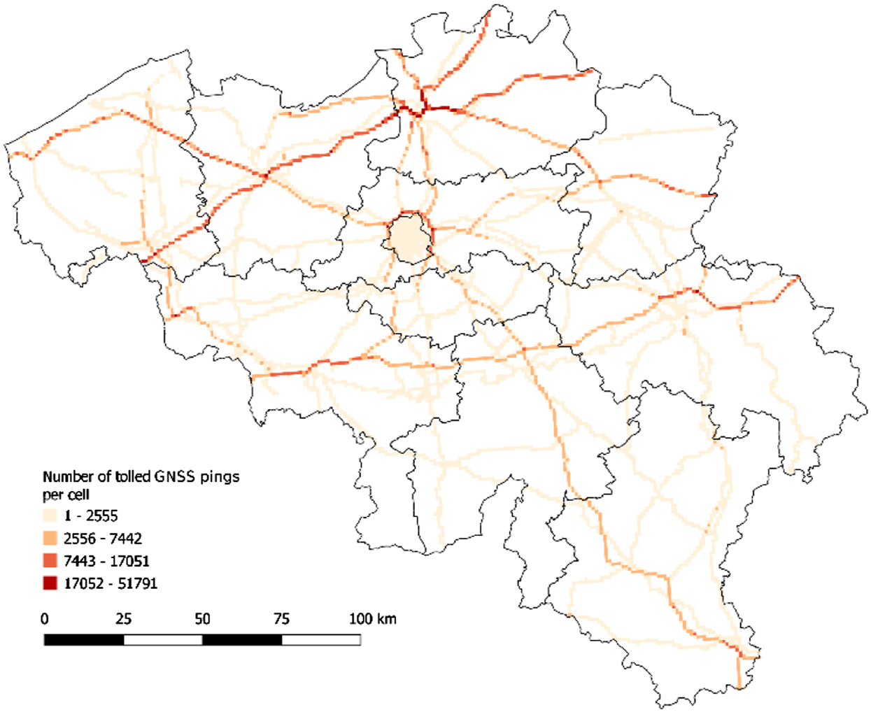
Total number of tolled GNSS pings per cell (10 Mio interBe trucks).

Figure 3.

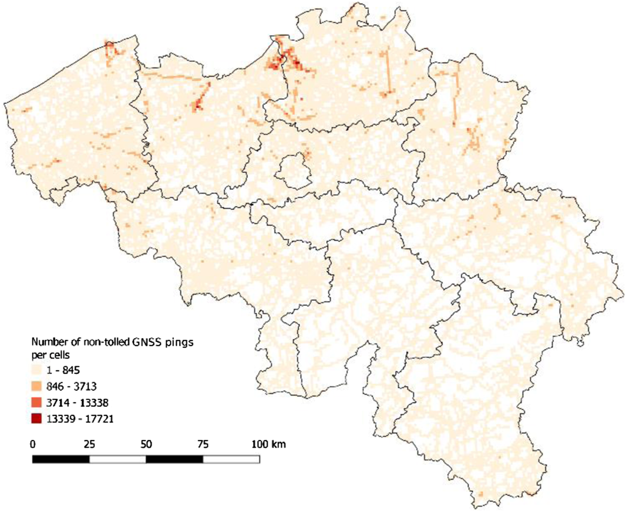
Total number of non-tolled GNSS pings per cell (3 Mio interBe trucks).

Figure 4.

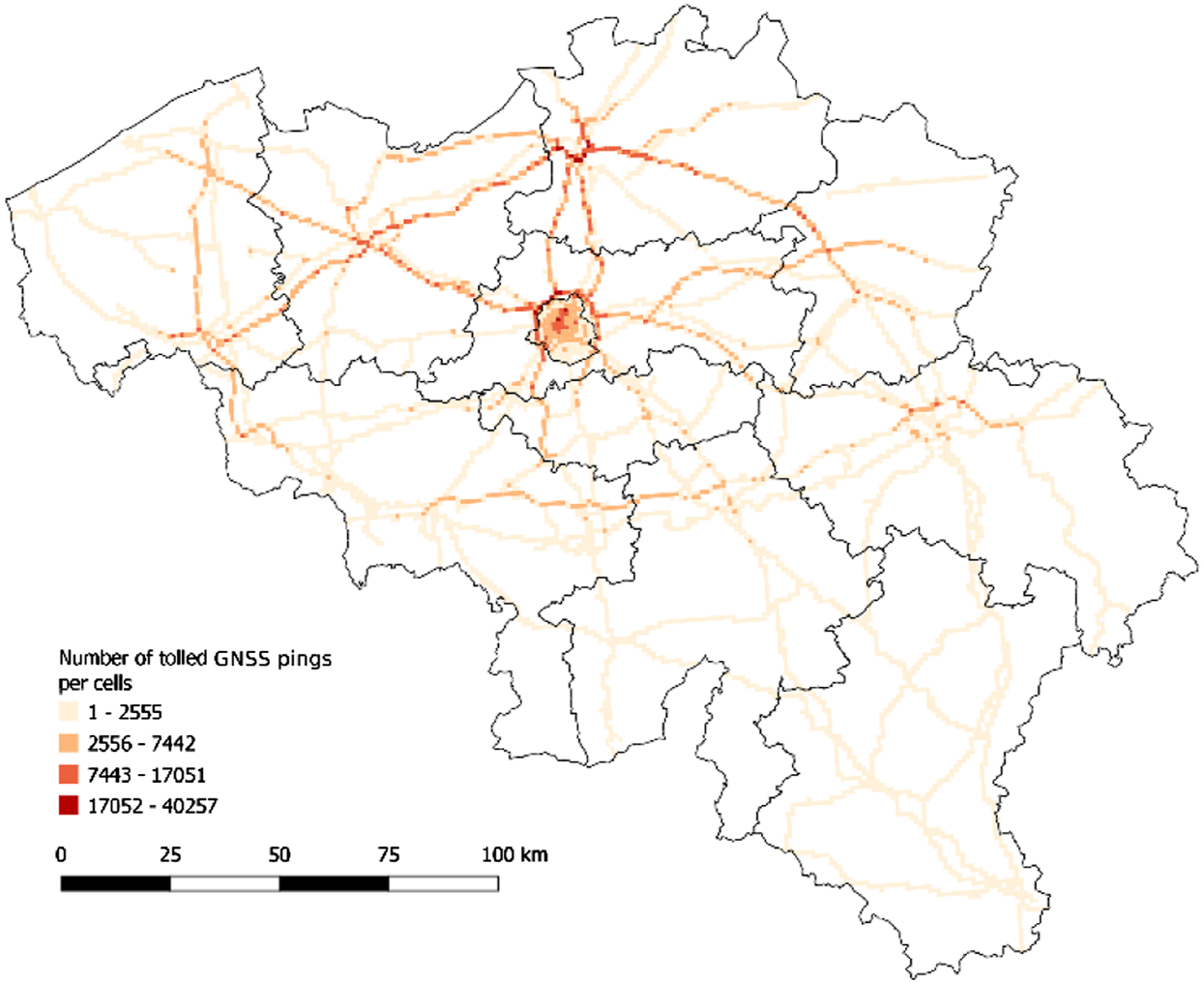
Total number of tolled GNSS pings per cell (8 Mio intraBe trucks).

Figure 5.

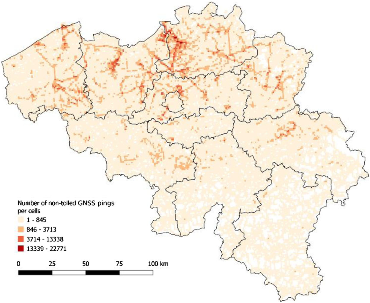
Total number of non-tolled GNSS pings per cell (10 Mio intraBe trucks).

International traffic on tolled roads (Figure 2) is mainly associated to major motorways and specifically in/around Antwerpen due to the port activity and the traffic with the Netherlands (E19 or E34) or France (E17 to Lille and E40 to Dunkerque). No concentration is observed in the BCR at the exception of the ring road (trucks bypassing the city). IntraBe trucks are undoubtedly observed on the same tolled road network (Figure 4), but are more concentrated near major cities (Brussels and Antwerpen) and also within Brussels. One might here expect deliveries by smaller trucks especially at centrally located firms (see Riguelle et al. 2007; Lebeau and Macharis 2014). Controlling the GCW of the trucks shows that small trucks are entering the BCR more than heavy ones (not illustrated here).

Thirteen million of pings are associated to non-tolled roads (see Table 3; Figures 3 and 5). They could of course be considered as a strong mismatch between distance charges and external costs. However, the location of these pings suggests why and where they are so numerous. These non-tolled truck movements are spread all over the country meaning that these movements are probably due to short movements such as parking, local access to firm, specific activities such as mining or quarrying, etc. Consequently, they are mainly emitted by intraBe trucks (10 Mio). Many concentrations appear in industrial zones and harbors especially as far as interBe trucks are considered. When looking at the interBe-trucks pings on non-tolled roads, port areas once again pop up (Antwerpen, Gent, Zeebrugge) as well as some well-defined portions of roads mainly in the Northern part of the country (associated to industrial activities), while non-tolled intraBe trucks (Figure 5) are characterizing many industrial areas in and around Flemish major cities (Antwerpen, Gent, Kortrijk) as well as some communications axes between those areas. In Wallonia values are less frequent and also characterize cities (Liège, Charleroi, La Louvière, Mons and Tournai). Let us remind that Figures 2–5 do not deal with distances, but with GNSS pings. These intra-regional spatial nuances are quite important to map in order to better understand policy choices and their consequences. Figure 3 and 5 are maps that could be considered for some suggestions of new road portions to be tolled in the future but also for understanding local or temporal specificities.

In other words, mapping the locations of the OBU’s emissions at a fine grain, enables to refine the rough and too simplistic north-south regional Belgian division. It shows that differences are mainly due to the urban network as well as to the location of industrial and commercial activities mainly at the outskirts of the cities. It also puts forward the importance of the ring roads around most cities and especially that around Brussels (out of the borders of the BCR) when tolling and evaluating external costs. Tolled pings are concentrated on the intercity road network, non-tolled pings reflect the location of the major economics activities and stops (see Adam et al. 2021 or Mérenne-Schoumacker et al. 2015).

Method

Drivers of the External Costs

External costs are the costs imposed on others and are not borne by the person/activity generating the costs. Their computation is here inspired by a EU study on external costs (European Commission 2019) and a more specific analysis in Flanders (Delhaye et al. 2017). Table 5 reports which drivers were considered for the estimation of the external costs of trucks. Some drivers are considered either as less relevant or could not be inferred from our database; they are coloured in red in Table 5. Climate damage is not considered here, as it can be internalized by the fuel tax. The computation is done at the level of each kilometre driven. Most categories of costs (congestion, pollution, noise, accidents) still raise conceptual difficulties for which we refer to the literature for full theoretical and/or estimation discussions (see European Commission (2019) for a literature survey). Our objective is to propose simple estimation rules and to include them in our evaluation.

Table 5.

Components for the Estimation of the External Costs of Trucks.

Type of road corresponds to the official Belgian classification into highways, major and local roads. Type of trucks is expressed in GCW and in Eurovalue.

The EU methodology also requires to differentiate external costs in function of an urban/rural classification, as population density is associated to air pollution, noise and/or accidents. The standard European procedure (Eurostat 2016) was here adopted: it is based on the classification of the NUTS3 regions. Unfortunately, this classification does not fit with our 1 sq km cells (Figures 3 and 4). To tackle this issue, we follow the Eurostat methodology. Each cell of our grid is characterized by its population density, that will then be the basis of the urban area. The urban area is defined as follows: (1) a concentration of contiguous cells having a density equal or higher than 300 habitant/km² and (2) a total population of over 5000 inhabitants. All cells not included in this “urban” group are labelled “rural” (Figure 6).

Figure 6.

Urban and rural areas in Belgium based on Eurostat (2016).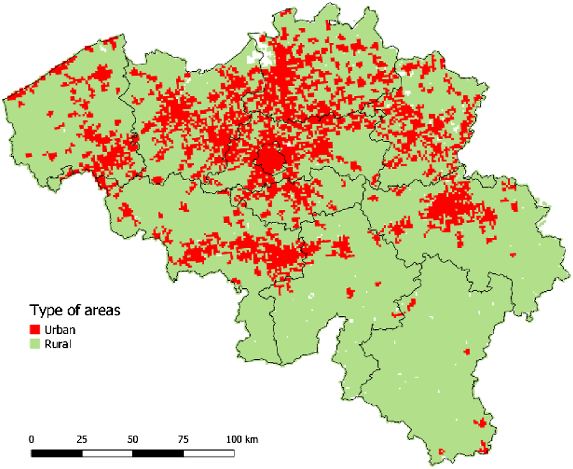

Traffic situation corresponds to the intensity of the traffic measured on a specific area (Christidis and Rivas 2012). In order to better capture the ‘real’ traffic situation rather than a local event that may introduce some noise (for instance, an accident), we decided to apply our computation on multiple days instead of only the 15^th of November (as a gentle reminder, please note that our original sample contains an entire week of data). The traffic situation is measured for each 1 km² cell of our grid, using the GNSS locations of the OBUs over the different hours of the day for all 5 days of the week (including our sampled day). For each cell, an average hourly speed is computed by aggregating the five working days and distinguishing peak and off peak hours (average hourly speed between 08:00 and 09:00 considers all the GNSS pings emitted during that hour for the 5 days), as well as the maximum observed. The latter value is considered as the speed for which trucks drive without any impediment to the circulation. These two computations should respect two conditions: (1) only cells containing a minimum of 600 GNSS points are considered, and (2) the hourly average speed is only calculated for hours containing a minimum of 50 GNSS points. Once the average hourly speed and the maximum speed are computed for each cell, four levels of traffic situation are provided for each hour: (1) “not congested” when the hourly average speed is higher than 80% of the maximum speed, (2) “near capacity” when the hourly average speed is between 66% and 80% of the maximum speed, (3) “congested” when the hourly average speed is between 33% and 66% of the maximum speed, and finally (4) “over capacity” when the hourly average speed is lower than 33% of the maximum speed (see Table 7 and Figure 7).

Figure 7.

Traffic situation in Belgium at 07:00 am.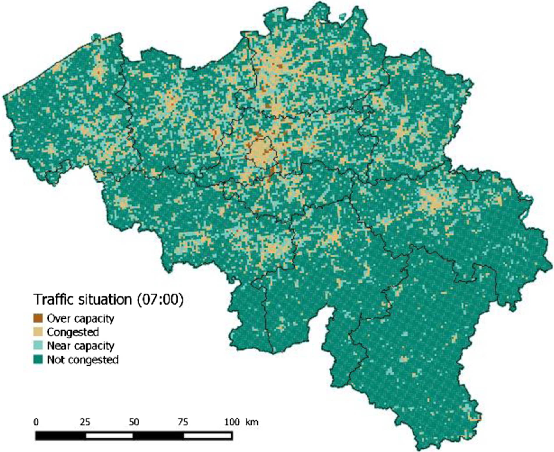

Time corresponds to the period of the day when the truck is moving (Day = between 06:00 and 22:00 – Night otherwise).

Definition of the External Costs

We here use external cost information either expressed per truck (congestion, accidents, infrastructure wear and tear) or per ton-kilometer (air pollution and noise). As the distance tax is paid per truck we also need to express the external costs per truck. For the external costs expressed per ton-kilometer, we use average load factors for the different categories of trucks (see Table 7 that presents the load factors used in this contribution, and largely inspired by the handbook of the European Commission (2019)). These load factors correspond to the theoretical average load carried by a given truck. This is required in our computation since trucks are not always driving in full capacity and their loads vary depending on their deliveries.

External congestion cost is here defined as the additional time that one more truck kilometer generates for all the other users of the road. Most of the methodologies use an estimated volume-speed curve for different types of roads, the number of vehicles observed on these roads, and look at the first derivative (see European Commission 2019). This decrease in speed is then translated into a loss of time for all the other road users. We rely on the European Commission (2019) estimates for each road type and the capacity of the road (Table 6).

Table 6.

Congestion Costs Common to all GCW Larger Than 3.5 T (€/100 km).

Traffic	Urban Roads (trunk roads and Highways)	Local Urban Roads	Rural Motorways	Rural Roads
Over capacity	64.2	132.6	58.7	92.7
Congested	49.5	116.4	45.3	79.2
Near capacity	34.9	94.4	31.9	62.3
Not congested	0	0	0	0

Environmental costs (air pollution) are the best understood category of transport external costs (see European Commission 2019). We know that their effect is significant, that they are site specific and depend on the type of car technology and fuel. A table with all values of air pollution costs per ton-kilometer (noted Tkm) used is reported in Appendix A. The average load factors are taken from Table 7.

Table 7.

Load Factors Used to Compute the External Costs of air Pollution and Noise.

GCW	Load Factors
[3.5 – 7.5]	3.41
[7.5 – 16]	9.33
[16 – 32]	11.48
[32 - ∞]	19.23

As system externalities are difficult to define and to use for road accident costs, we take into account the effects of a small variation in the volume of trucks on the risks of accidents and their costs, where the costs include, first the value of the lives that are lost, second the subjective costs of non fatal accidents, and third the material costs. We here limit ourselves to the two latter externalities that have two aspects. First, when a vehicle participates in traffic flow, it generates a potential accident risk for itself, risk that is not fully taken into account due – among others – to insurance and social security coverage of medical costs. Second, by joining the traffic flow, the vehicle also influences the risk for the other vehicles. Using several assumptions (value of life, accident probabilities, behavioral parameters, etc.), Delhaye et al. (2017) estimate the following values of accident costs expressed in €/100 veh. km: 1.08 for motorways, 1.87 for urban roads and 2,97 for “other roads”.

Noise depends on traffic intensity (decreasing marginal external cost), on the period of the day (day/night) and on the population density along the roads (urban/rural). We here once again rely on the European Commission (2019) estimates. Values per ton-kilometer are reported in Appendix B and load factors are to be found in Table 7.

The external infrastructure cost is the additional maintenance cost caused by an additional vehicle. The marginal infrastructure cost depends mainly on the axle weight (GCW) that causes most deformations of the road surface. According to the literature (see e.g. Newbery 1988) the marginal infrastructure costs are much lower (half) than the average infrastructure cost. The European Commission handbook (European Commission 2019) suggests 7€/1000 Tkm for a large truck, and 2 €/1000 Tkm for a small truck. Since the marginal cost is expressed in Tkm, the computation requires a loading factor. For the Flemish Region, Delhaye et al. (2017) propose 3.83 tons for trucks having a GCW between 3 and 12 T, and 1025 for trucks having a GCW between 12 and 40 T. By doing so, the marginal external infrastructure cost for ‘light’ trucks (3.5–12 T) and ‘heavy’ trucks respectively correspond to 0.766 and 7175 euro/100 veh. km.

Computation of the External Costs: An Illustration

As our data base gives a detailed information on the itinerary of trucks, we propose to illustrate the evolution of the external costs under specific spatio-temporal conditions. To do so, Figure 8(a) and (b) compute the external costs for two trucks on one itinerary (Figure 8(a) and (b). Each hour is characterized by a specific traffic situation, a type of road and its location in a rural or urban environment. In addition, the day starts at 06:00 and the night starts at 22:00. Finally, the two trucks drove the same number of kilometers for each hour. Truck A has a GCW of 10 tons and a Eurovalue of II, while truck B is heavier (GCW of 34 tons) and has a much favorable Eurovalue (VI). In other words, truck B has a much greener engine which generates less pollution: Airpol is indeed less present on Figure 8(b) compared to Figure 8(a).

Figure 8.

24 hours externality costs for 10 km driven by (a) Truck A (GCW 10, Eurovalue II) and (b) Truck B (GCW 34, Eurovalue VI).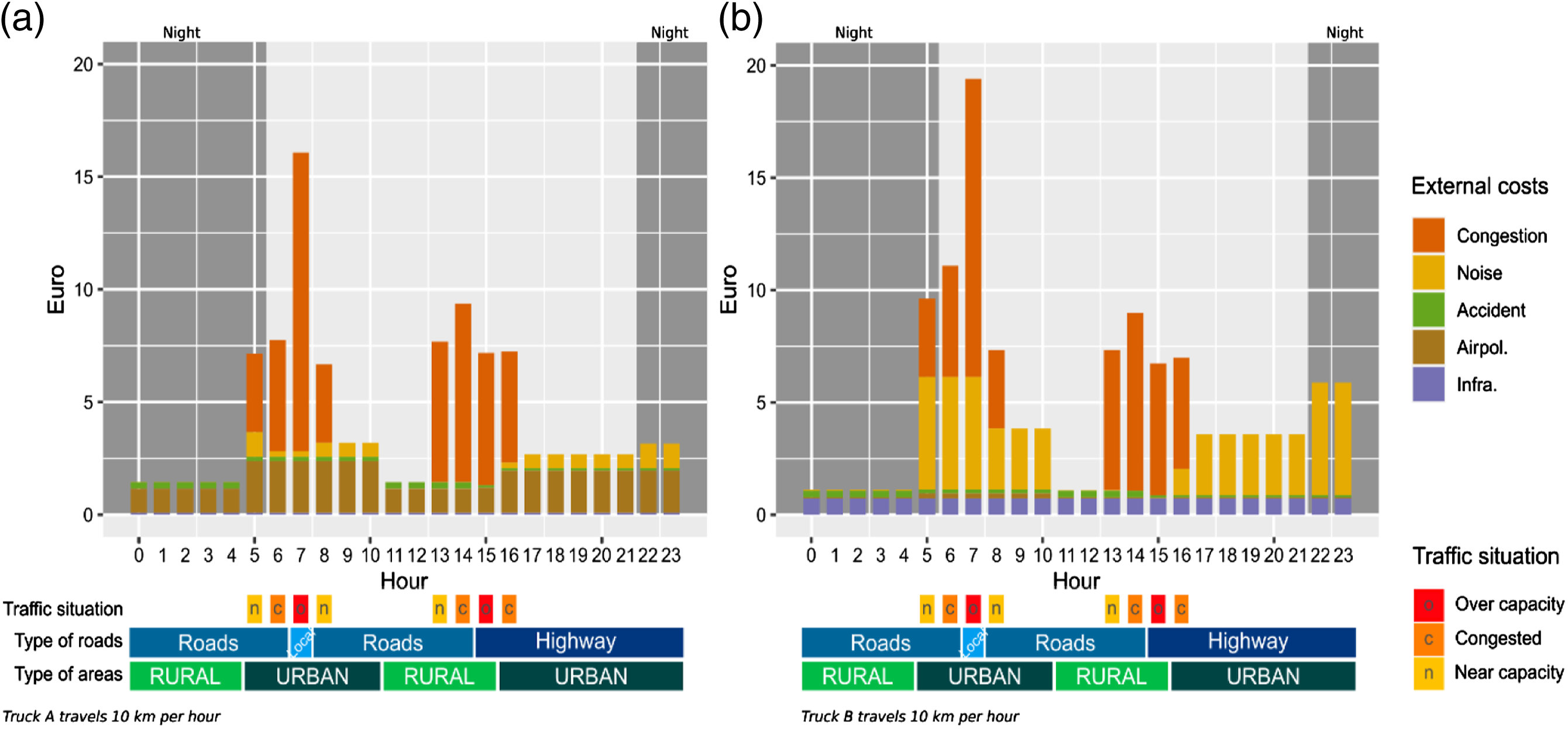

Variations in type and amount of externality costs are due to several factors such as the use of different types of roads (infrastructure and accidents), the hour (congestion), the area (noise and air pollution) as well as the type of trucks (smaller but more polluting – A – or larger and cleaner – B). They consequently vary in time and place as stated by Figure 8. Congestion costs are highly associated with traffic situation, type of road and urbanity of the area surrounding the road. Noise costs depend indeed on the traffic conditions, the urbanity of the area and the time of the day. Theoretical variations proposed in Figure 8(a) and (b) are completely in phase with the literature (European Commission 2019).

Result

A good correspondence between distance tolls and external costs requires two properties: first, the toll paid for a trip should be equivalent to the external costs of that trip. Second, the structure of the external costs should match the characteristics of the truck trip so that the best type of truck is used on the right trajectory, at the best time of the day.

Costs and Revenues

In our 1-day cleaned sample, 91,199 trucks (ID) emitted 31.5 Mio OBU pings. The total distance covered by these trucks was estimated to 13.5 Mio kilometers. 73% of these kilometers were tolled, which leads to a total toll revenue of 1.4 Mio euros. To compute the total toll revenue, each truck has been considered individually based on the characteristics of the vehicle and the trip (see Table 1 for more details about the calculation). The fact that only 75% of the kilometers travelled in Belgium were tolled could be seen as an important mismatch between tolls and external costs. As explained previously, most of the major roads are tolled, but there are still roads free of tax used for access to ports and activities, for deliveries or for alternative itineraries.

When computing the external cost of the 91,199 trucks driving on the tolled roads in Belgium, we see that they are much higher than the total toll paid (Table 8). As explained in the preceding sections, EU regulation does not allow that the total toll revenues exceed the infrastructure costs. From our estimation, it would appear that Belgium violates the EU legislation, because the toll revenue is twice as high as the infrastructure cost. However, two reasons/interpretation of the legislation may explain this violation. First, the Belgium KCS tolls the trucks based on their characteristics and not on their actual loads. As described above, most of the trucks circulating in Belgium are larger than 32 tons (Table 3), and are then tolled at a higher rate (see the categories in Table 1). However to compute the infrastructure costs for this category of vehicles (>32 tons), this paper uses a loading factor of 10.25 tons instead of considering the maximum capacity as is done in the Belgium KCS (32 tons). This difference of 20 tons may explain the difference between the external cost and the toll computed. These two ways to interpret the European legislation about the load of the vehicles produce different values. Half of the trucks circulating in Belgium are international ones: one may easily hypothesize that these trucks are driving more often in full capacity than the intra-national ones. Second, infrastructure costs may also be interpreted in a way that it includes structures that help reducing the impact of noise, and not only the infrastructure damages to the roads. This may lead to a toll based on a higher coefficient for infrastructure costs than the one developed by the European Commission.

Table 8.

External Costs and Toll Revenue.

Type	Euro
Congestion costs	351,798 €
Air pollution	769,143 €
Accident costs	110,800 €
Noise costs	2,418,119 €
Infrastructure costs	700,282 €
Total external costs	4,350,142 €
Total toll revenue	1,442,035 €

Although the toll is higher than the infrastructure cost, it is smaller than the sum of all the external costs (4.35 Mio €). Noise and air pollution costs dominate the external costs, which is expected in a densely populated country and in the method use for estimating noise (European Commission 2019). In Belgium, the Regions count on the toll revenues to pay for infrastructure. We see that this is indeed the case, but the toll revenues are clearly much lower than the total external costs of trucks. This really calls for a deeper analysis of the distance tax.

Assessing the Structure of the Distance Tax

The total toll (revenue) is now compared to externality costs (Figure 9) for a set of categories mentioned in Tables 2 and 5. For the ease of comparison, taxes and costs are expressed in euros per kilometer driven by a truck¹ (€/veh.km).

Figure 9.

Toll (revenues) and externality costs expressed in €/veh.km.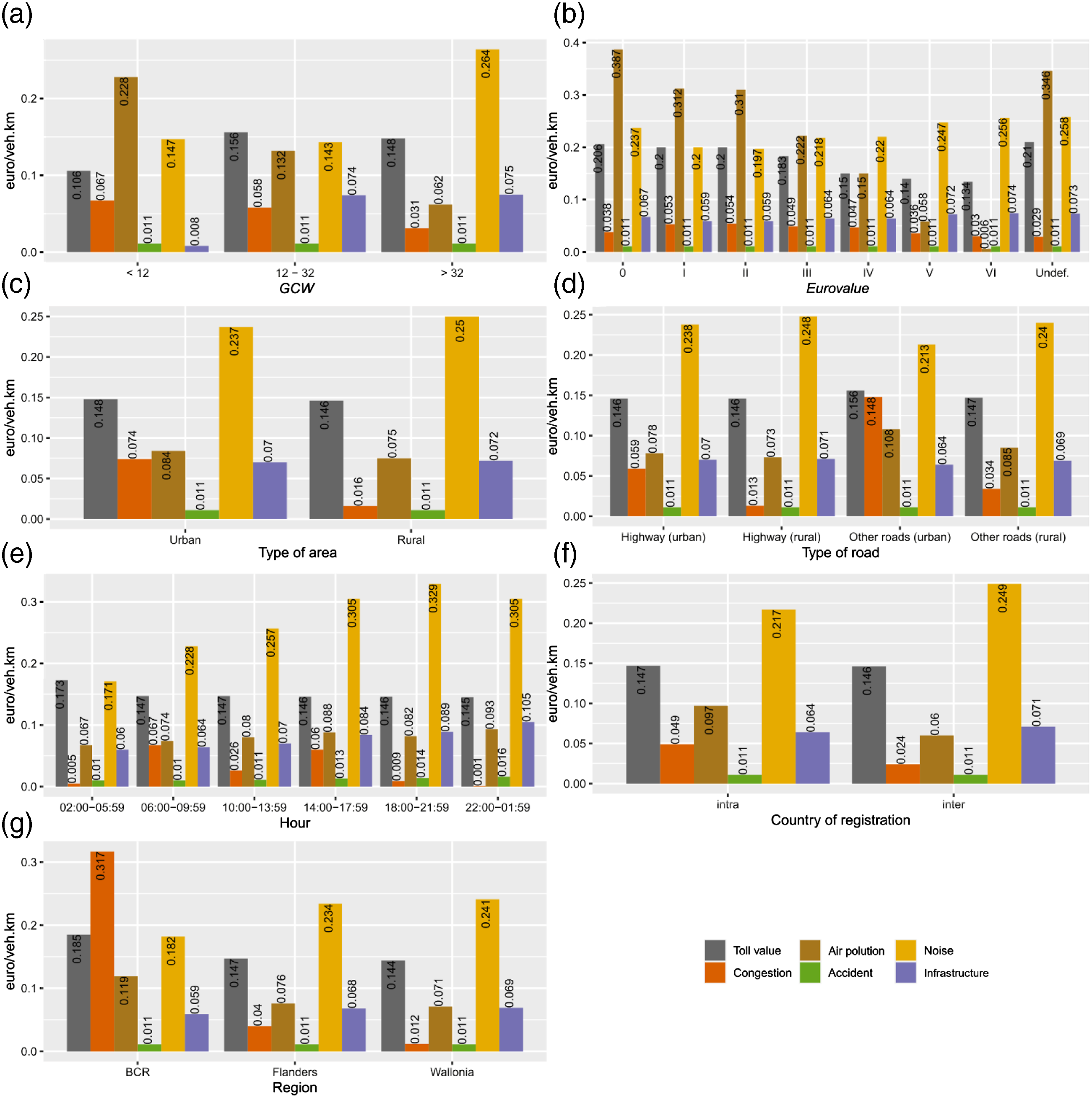

We know that the biggest trucks (GCW > 32 T) represent 73% of our 1-day sample of trucks (see Table 3). So, although these trucks pay higher total tolls (see Table 1), this does not compensate for the much larger noise costs. An interesting observation is that study shows that large diesel trucks are the greatest contributors to black carbon emission (Wang et al., 2018). However, when estimating the pollution emitted compared to the capacity of the truck, small trucks are relatively more polluting (Figure 9(a)) expressing that “vehicle types matter more than traffic volume for near-road air pollution”. (Wang et al., 2018). Figure 9(b) presents the same trend: trucks equipped with greener engines (Eurovalues IV, V and VI) are indeed linked with a smaller value of air-pollution costs, but with a larger cost of noise.

Figure 9(c) and (d) show that there is no big difference between urban and rural areas, as well as with the type of road (highway or not). Only congestion costs are much higher in urban areas, indeed linked with the traffic situation found around cities that concentrate economic activities. Two peaks in the cost of congestion are observed through the day (Figure 9(e)), one in the morning (between 06:00 and 10:00), and the second one in the afternoon (14:00 to 18:00).

Furthermore, the variation over time brings other insights (Figure 9(e)). Firstly, the value of the toll is higher early in the morning (before 06:00), because the tolled network is more intensively used. Indeed, trucks (1) aim to deliver goods before the opening hours (distribution, groceries, construction or industrial sector), and/or (2) simply organise their trips to avoid being stuck in the rush hour in the morning. Secondly, the infrastructure cost is more important in the afternoon and evening than in the morning. As infrastructure costs depend on the size of the truck only, this second point explains that trucks driving in mornings and early afternoon periods vary in size, while bigger trucks are more intensively used in afternoons and evenings. Figure 10 shows that between 02:00 and 05:59 the shares of small, medium and big size trucks are respectively 14, 17 and 69% while, after 18:00 figures are respectively 6, 8 and 86%. Indeed, during the working hours (mostly from 08:00 to 17:00), different types of trucks (from small vans to large trucks) are delivering various type of goods (e.g., mail, boxes, food to a local butchery or construction materials to a building site). On the contrary, trucks that are circulating after working hours are bigger trucks crossing Belgium to join other countries. Figure 11 shows that most of the trucks driving in the morning and early morning are intraBe trucks (around 60%) while late afternoons and evenings is dominated by interBe trucks (around 60%). Because intraBe trucks are driving during working hours, they are then more confronted to congested areas than interBe trucks (that could just cross the Belgian territory without exiting the highways). It results that intraBe trucks have higher congestion costs (Figure 9(f)). In addition, interBe trucks are also more driving on highways located in more rural areas, hence avoiding traffic jams appearing in and around the major city centers (Figure 9(d)). Finally, intraBe trucks cause more air pollution than interBe ones. One explanation is that Belgian trucks are less green than international ones (Table 3), and are more driving in urban areas. This goes with the same conclusion drawn by Frank and Engelke (2005) and saying that our urban areas have moved from air pollution created by industries to air pollution generated by vehicles. In the case of the BCR, regional planners and policy makers should be aware of this to enhance the air quality in the city. This is also valid for the CO2 emissions at the level of the Region, but with a different aspect. Most of the CO2 contributions in urban areas are made by people attracted by the city, but are not residing there (Perumal and Timmons 2015).

Figure 10.

Number of trucks by category of GCW and by hour.

Figure 11.

Number of intraBe and interBe trucks by hour.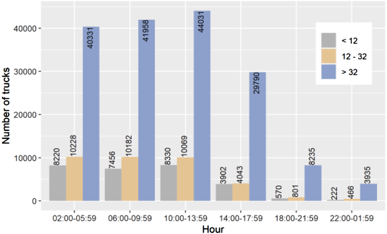

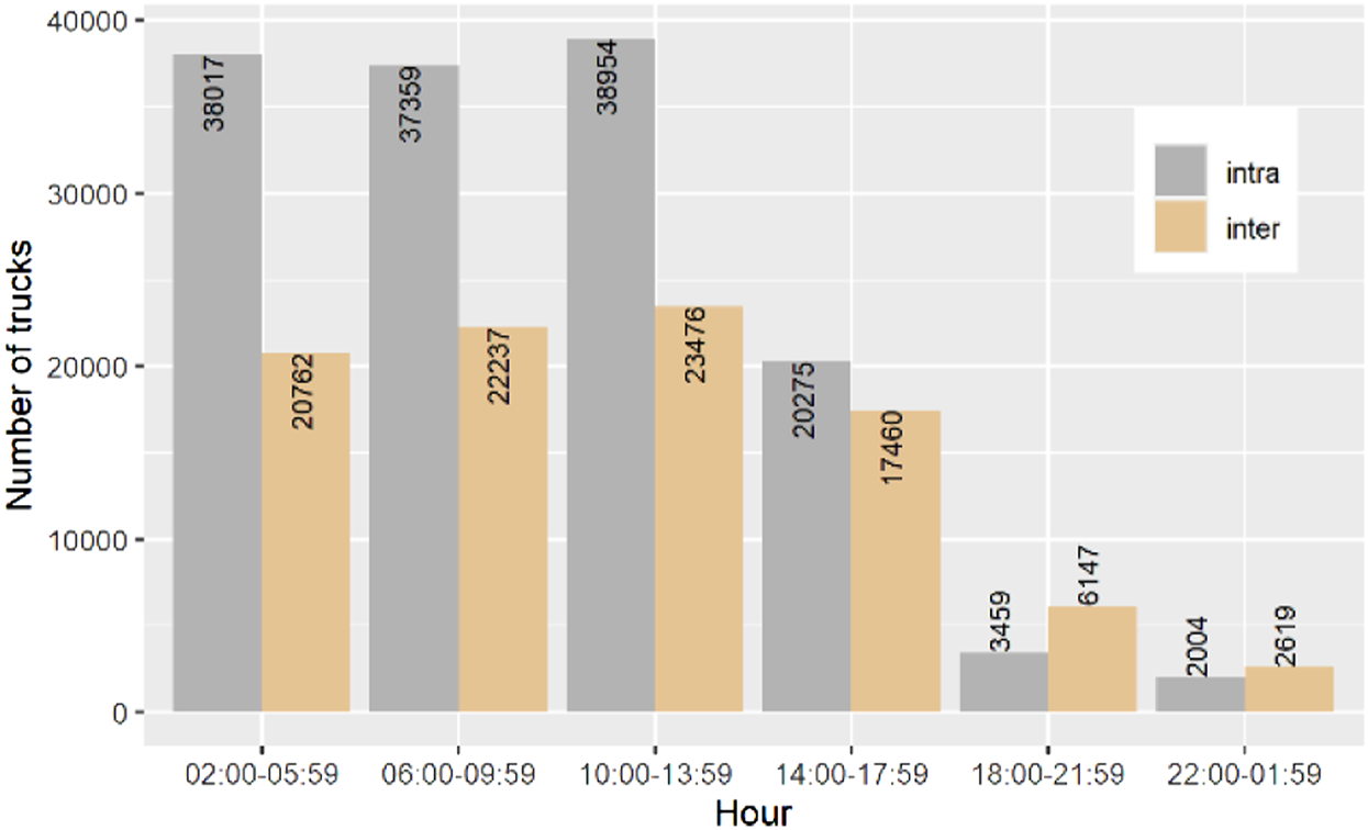
Figure 9(g) shows the distribution of the relative toll and external costs for each of the three Regions. Noise cost is the major external cost for Flanders and Wallonia, while congestion is dominant in the BCR. One has here to remind that BCR is fully urban (while Flanders and Wallonia both correspond to more diversified urban realities with hierarchised urban networks and also major green areas). It is well known that computing a regional average hides the many transport and human realities. In comparison, the BCR corresponds to the centre of Brussels (not its suburbs), which consequently attracts smaller vans better adapted to deliveries in urban environment (Lebeau and Macharis 2014).

Figure 12 goes beyond the simple regional differences: it gives the differences between revenues and external costs by 1sq km cell. We know the difference is always negative (revenues are smaller due to EU parameter choices); hence the values in these two maps are centred. Regional differences (Figure 9(g)) hide major local differences already discussed above. In other words, applying one rule at a macro level (country, region) hides important spatial differences due to the economic, human or infrastructure realities.

Figure 12.

Difference between toll and total externality costs on the tolled road network, for (a) interBe and (b) intraBe trucks (values centred to the mean) – euro/km².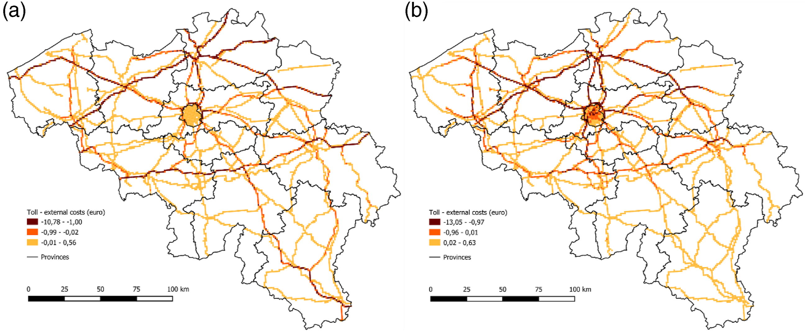

Conclusion and Discussion

The distance toll is a major tool to make trucks contribute for the wear and tear of the road infrastructure and pay for their external costs. Even if this tolling system is not yet adopted by all EU countries, it is expected to be used more and more frequently as trucks will become more fuel efficient in the future. Amongst others, low-emission zones, climatic challenges and developments of new technologies are key elements that will change the current characteristics of freight transportation in the near future.

This paper assesses how and where distance tolls match external costs. As the damage of external costs depends on the combination of the type of vehicle and the exact time and location of their use, it is important to exploit detailed time and location data to compute both the external costs and the toll revenues. A 1-day sample of GNSS pings for all tolled and non-tolled roads in Belgium has been used in this paper to compute the external costs set up by the European Commission. Although such new “big” data have major limitations, mainly associated to the data cleaning process (Finance et al. 2019), their use allows to conduct analyses at fine-grained scale and provide clear support for more efficient policy choices. The results of our analysis can be summarized as follows.

First, the toll is in general much lower than the sum of all the external costs. The reason is that the EU has limited the total toll revenues to the infrastructure costs. This limit prevents tax exporting by transit countries, and also explains why other taxing systems, such as urban congestion tolls, are also implemented (e.g. in London, Stockholm, Goteborg).

Second, the toll structure is mainly based on two parameters that are officially recognized as the most relevant criteria for differentiation of external costs: vehicle weight (GCW) and conventional pollution emission standard (Eurovalue). However, our analysis suggests that noise and congestion costs appear to be far more important. This implies that, for instance, new heavy trucks with the best air pollution abatement infrastructure pay a relatively small toll compared to the large noise and congestion costs that they produce. Addressing this mismatch will require several policy actions. On the one hand, there is a need for a toll that better matches the noise costs generated by trucks, which have been shown to create not only discomfort but also health damages (Cantuaria et al. 2021). Some specific infrastructures (such as walls and vegetation) along the transportation network help to reduce the external noise (Jacyna et al. 2017). Since this mitigating effect could not be included in our computations, we may have over-estimated the noise cost, as well as under-estimated the value of the infrastructure cost. On the other hand, the toll may also need to be varied as a function of the level of congestion, especially for the BCR that concentrates major economic activities. However, this only makes sense when cars are also tolled in function of the congestion, because an increase in car use will compensate the efforts of trucks to reduce their activity (Calthrop et al. 2007). Indeed in most of the countries, commuters do not pay for the congestion costs although they are the main responsible group (Brueckner 2000).

Overall, our analysis provides a detailed picture of how the toll paid by trucks compares to their external costs. However, two issues should be considered. The kilometer tax is only paid by trucks having a gross vehicle weight of over 3.5 tons. But in recent years, the number of small trucks (<3.5 T) has substantially increased, also due to the growth of e-commerce (Beckers et al. 2018). It would be interesting to complement our findings with information on the trajectories of these small trucks and analyze the patterns of substitution between large and small trucks possibly induced by the toll (de Bok et al. 2020). In addition, this paper shows that numerous GNSS pings are located on non-tolled roads, such as in harbors, in economic/commercial activity zones, or within cities (at the exception of BCR). This could point to an adaptation of the tolled network, in as far as the installation and transaction costs can be justified.

In conclusion, distance tolls for trucks are a political compromise and an important source of revenues, but tolling in function of location and time is crucial to keep the external costs of trucks under control. Values put forward in this paper are, of course, highly dependent upon the EU report (2019), but the paper suggests reliable orders of magnitude that should inspire policy makers in setting national/regional/local priorities in terms of freight transport. This is particularly relevant in light of the many challenges related to the rising importance of ecological issues, the increase in demand for energy, and the development of new technologies. For instance, in spite of the availability of new energy sources (electricity and hydrogen are two currently debated options), which may reduce the impact of trucks on the environment, our current eurovalue classification will certainly become obsolete. In addition, thanks to better technologies, vehicles may become less noisy. Although their external costs linked with noise will reduce, these trucks are typically heavier and may have a bigger impact on the infrastructure. These are only a few examples of the issues that planners should be aware of in order to propose better policies and develop a more forward-looking spatial planning.

Footnotes

Declaration of Conflicting Interests

The author(s) declared no potential conflicts of interest with respect to the research, authorship, and/or publication of this article.

Funding

The author(s) disclosed receipt of the following financial support for the research, authorship, and/or publication of this article: This work was supported by the Fonds De La Recherche Scientifique - FNRS; PDR T022719

ORCID iD

Arnaud Adam

Note

Air Pollution Cost (€/100 Ton-km) by GCW,Type of Area and Road

GCW	Eurovalue	Urban Motorway	Urban Other Road	Rural Motorway	Rural Other Road
<7.5 t	0	15.44	18.35	9.19	8.71
<7.5 t	I	10.57	11.17	6.32	5.66
<7.5 t	II	10.35	10.78	6.2	5.58
<7.5 t	III	7.54	9.18	4.54	4.22
<7.5 t	IV	5.28	5.77	3.21	2.93
<7.5 t	V	2.37	7.2	1.49	1.59
<7.5 t	VI	0.28	1.48	0.26	0.36
7.5 - 12 t	0	9.07	11.58	5.39	5.26
7.5 - 12 t	I	5.49	7.06	3.27	3.18
7.5 - 12 t	II	5.51	6.77	3.29	3.14
7.5 - 12 t	III	3.99	5.68	2.39	2.46
7.5 - 12 t	IV	2.73	3.49	1.65	1.67
7.5 - 12 t	V	1.28	4.53	0.79	0.93
7.5 - 12 t	VI	0.18	0.66	0.14	0.18
12 - 14 t	0	5.1	6.98	3.03	3.02
12 - 14 t	I	3.1	4.28	1.84	1.84
12 - 14 t	II	3.1	4.14	1.85	1.82
12 - 14 t	III	2.3	3.57	1.38	1.44
12 - 14 t	IV	1.54	2.2	0.93	0.98
12 - 14 t	V	0.74	2.66	0.45	0.56
12 - 14 t	VI	0.1	0.35	0.08	0.1
14 - 20 t	0	5.66	8.58	3.36	3.5
14 - 20 t	I	3.36	5.25	1.99	2.1
14 - 20 t	II	3.43	5.04	2.04	2.08
14 - 20 t	III	2.56	4.4	1.53	1.68
14 - 20 t	IV	1.74	2.63	1.04	1.12
14 - 20 t	V	0.85	3.61	0.52	0.87
14 - 20 t	VI	0.11	0.48	0.08	0.12
20 - 26 t	0	2.74	4.43	1.62	1.75
20 - 26 t	I	1.96	3.25	1.16	1.25
20 - 26 t	II	1.98	3.1	1.18	1.24
20 - 26 t	III	1.56	2.64	0.93	1
20 - 26 t	IV	1.05	1.6	0.63	0.67
20 - 26 t	V	0.48	1.98	0.29	0.45
20 - 26 t	VI	0.05	0.24	0.04	0.06
26 - 28 t	0	2.03	3.26	1.19	1.29
26 - 28 t	I	1.44	2.38	0.85	0.92
26 - 28 t	II	1.46	2.3	0.87	0.92
26 - 28 t	III	1.13	1.93	0.67	0.73
26 - 28 t	IV	0.76	1.18	0.46	0.48
26 - 28 t	V	0.32	1.45	0.19	0.32
26 - 28 t	VI	0.04	0.17	0.03	0.04
28 - 32 t	0	1.89	2.94	1.11	1.2
28 - 32 t	I	1.37	2.21	0.81	0.88
28 - 32 t	II	1.37	2.1	0.81	0.86
28 - 32 t	III	1.05	1.75	0.63	0.68
28 - 32 t	IV	0.71	1.09	0.42	0.45
28 - 32 t	V	0.27	1.23	0.16	0.25
28 - 32 t	VI	0.04	0.13	0.03	0.04
>32 t	0	1.63	2.69	0.96	1.04
>32 t	I	1.18	2.01	0.7	0.76
>32 t	II	1.19	1.91	0.71	0.75
>32 t	III	0.93	1.6	0.55	0.61
>32 t	IV	0.63	0.99	0.38	0.4
>32 t	V	0.26	1.1	0.16	0.23
>32 t	VI	0.03	0.12	0.02	0.03

Noise Cost (€/100 Ton-km)

GCW	Time	Congestion	Urban	Rural
[3.5 - 7.5]	Day	Congested	1.5	0.01
[3.5 - 7.5]	Day	Not congested	3.6	0.03
[3.5 - 7.5]	Night	Congested	2.7	0.02
[3.5 - 7.5]	Night	Not congested	6.5	0.05
[7.5 – 16]	Day	Congested	0.7	0.01
[7.5 – 16]	Day	Not congested	1.8	0.01
[7.5 – 16]	Night	Congested	1.3	0.01
[7.5 – 16]	Night	Not congested	3.2	0.02
[16 – 32]	Day	Congested	0.6	0
[16 – 32]	Day	Not congested	1.3	0.01
[16 – 32]	Night	Congested	1	0.01
[16 – 32]	Night	Not congested	2.4	0.02
≥ 32	day	Congested	0.6	0
≥ 32	day	Not congested	1.4	0.01
≥ 32	Night	Congested	1.1	0.01
≥ 32	Night	Not congested	2.6	0.02

References

Adam

Finance

Thomas

2021. “Monitoring Trucks to Reveal Geographical Structures and Dynamics: From GNSS Traces to Spatial Interactions,” Journal of Transport Geography 91: 102977. DOI: 10.1016/j.jtrangeo.2021.102977.

1991. “Building a Strategic Model for Edinburgh”. Proceedings of Seminar D, PTRC Summer Annual Meeting. London: PTRC.

Beckers

Cárdenas

Verhetsel

2018. “Identifying the Geography of Online Shopping Adoption in Belgium.” Journal of Retailing and Consumer Services 45: 33-41. DOI: 10.1016/j.jretconser.2018.08.006 .

1997. External Costs of Transport in Externe. Final Report. Stuttgart: IER.

Broaddus

Gertz

2008. “Tolling Heavy Goods Vehicles: Overview of European Practice and Lessons from German Experience.” Transportation Research Record 2066: 106-113. DOI: 10.3141/2066-12 .

Brueckner

Jan K

. 2000. “Urban Sprawl: Diagnosis and Remedies.” International Regional Science Review 23 (2): 160-71. DOI: 10.1177/016001700761012710 .

Calthrop

De Borger

Proost

. 2007. “Externalities and Partial Tax Reform: Does it Make Sense to Tax Road Freight (but not Passenger) Transport?” Journal of Regional Science 47, 4: 721-52. DOI: 10.1111/j.1467-9787.2007.00520.x .

2021. “Residential Exposure to Transportation Noise in Denmark and Incidence of Dementia: National Cohort Study.” BMJ 374: n1954. DOI: 10.1136/bmj.n1954 .

Christidis

Rivas

2012. “Measuring Road Congestion.” Institute for Prospective Technological Studies (IPTS), European Commission Joint Research Centre. DOI: 10.2791/15282 .

2020. ““Exploring the Impacts of an Emission Based Truck Charge in the Netherlands”.” Case Studies on Transport Policy 8 (3): 887-94. DOI: 10.1016/j.cstp.2020.05.013 .

11.

De Borger

Proost

. 2017. “What can European Experience Teach Us for Belgian Transport Policy.” Reflets et perspectives de la vie écoconomique, LVI: 33-53. https://www.cairn-int.info/article-E_RPVE_562_0033–what-can-european-experience-teach-us.htm

12.

Delhaye

De Ceuster

Vanhove

Maerivoet

. 2017. “Internalisation of External Costs of Transport in Flanders.” Reflets et perspectives de la vie économique, tome LVI 2017 (3): 55-74. https://www.cairn-int.info/journal-reflets-et-perspectives-de-la-vie-economique-2017-2-page-55.htm

13.

Doll

Schaffer

2007. “Economic Impact of the Introduction of the German HGV Toll System.” Transportation Policy 14: 49-58. DOI: 10.1016/j.tranpol.2006.09.001.

14.

European Commission . 2019. “Handbook on the External Costs of Transport.” Publications Office of the European Union, Directorate-General for Mobility and Transport: 348.

15.

European Parliament . 2018. “Road Charges in the EU: A Fairer and Environmentally Friendlier System.” Press News. https://www.europarl.europa.eu/news/en/headlines/society/20181018STO16586/road-charges-in-the-eu-a-fairer-and-greener-system

16.

Eurostat . 2016. “Urban-Rural Typology.” https://ec.europa.eu/eurostat/fr/web/rural-development/methodology

17.

Eyre

N.J.

Ozdemiroglu

Pearce

D. W.

Steele

1997. “Fuel and Location Effects on the Damage Costs of Transport Emissions.” Journal of Transport Economics and Policy 31: 5-24.

18.

Finance

Adam

Jones

Thomas

. 2019. “Révéler la Polarisation Économique d'une ville à Partir des Traces GNSS de Camions. Le cas de Liège”.” Bulletin de la Société Géographique de Liège 72: 95-114. https://hal.archives-ouvertes.fr/hal-03020567

19.

Frank

L. D.

Engelke

2005. “Multiple Impacts of the Built Environment on Public Health: Walkable Places and the Exposure to Air Pollution.” International Regional Science Review 28 (2): 193-216. DOI: 10.1177/0160017604273853.

2020. “Has Heavy Vehicle Tolling in Europe Been Effective in Reducing Road Freight Transport and Promoting Modal Shift?” Transportation 47 (2): 865-92. DOI: 10.1007/s11116-018-9922-3 .