Militarized Conflict,Trade,and Economic Development in a Structural Equation Model With Spatial Considerations

Abstract

While conflict pervades virtually every aspect of society, there have been relatively few crossovers between Regional Science and Peace Science. This paper pays tribute to Walter Isard, pioneer of peace science research, and Kieran Donaghy, who has contributed to research on arms race dynamics and macroeconomic stability. We review studies that examine the impact of (i) trade on conflict, (ii) the economy on militarized disputes, and (iii) conflict on economic development. The analysis develops a structural equation model (SEM) to test the hypotheses simultaneously using the Correlates of War project data. Consistent with the liberal proposition, we found that the pacifying effect of trade is robust across alternative SEM specifications. Controlling for standard explanatory variables, the SEM estimates reveal that the indirect impact of economic development on conflict mediated by trade is statistically significant at the 0.1-percent level. Trade is, therefore, a critical intervening variable that transforms conflict-inducing economic expansion into a pacifying influence on militarized disputes. The spatial version of the SEM confirms that democracies do not attack each other. While trade does not appear to have a local spillover effect on conflict, proximity to neighboring democracies does lead to fewer conflicts. The final hypothesis argues that conflict affects national economic performance, which Donaghy refuted in his 1995 Conflict Management and Peace Science paper. Consistent with Donaghy’s finding, the estimates reject the claim that conflict disrupts economic stability. The conclusion section discusses the implications for Kieran Donaghy’s larger body of work.

Keywords

interstate conflict peace science history spatial analysis structural equation model trade

Introduction

If anything is certain, according to Isard (1975) in his Introduction to Regional Science, it is that conflict pervades all aspects of society. Isard (1992) later dove in with this bold statement, “The history of humankind and the rise and fall of civilizations is unquestionably a story of conflict. Conflict is inherent in human activities. It is omnipresent and foreordained” (p. 1). Despite the omnipresence of conflict in all aspects of life, Isard (1975) lamented that conflict did not receive the attention it deserves in the scholarly discourses. Isard contended that the state of the social sciences at that time was such that conflict often received, at most, a passing consideration and, sometimes, not at all. The need for peace research, coupled with escalating hostilities at the height of the Cold War, motivated Isard to convene the first meeting of the Peace Research Society in 1963 (Isard 2000). Isard’s vision–articulated in the 1963 meeting–of a multidisciplinary field utilizing empirical quantitative methods became the foundation of today’s Peace Science.

In Isard’s (1979) view, economic interdependence is at the center of human conflict. Since resources are finite, the welfare of one economic entity is dependent on the consumption and production decisions of other entities, and the reverse is also true. If one entity suffers a negative externality from another’s consumption or production decisions, the result could be armed conflict between the entities involved. Isard (2000) noted that preventing the outbreak of an international conflict had been the pursuit of several independent academics–each with their own research questions and empirical methods. This plurality is precisely how the Peace Science Society should be, according to Isard (2000), as a forum where scholars from multiple disciplines come together to stimulate each other and disseminate research findings. But despite the vision of a multidisciplinary area of inquiry, Isard approached dispute resolution primarily through the framework of general equilibrium modeling (Elhance 1993) because of his scholarship in neoclassical location theory. Because the founder’s modeling approach was developed by spatial scholars to examine questions about the location of economic activities, regional science evolved into a field that tends to focus more on the spatial aspect of the economy and less on the intersection of trade and conflict.

Indeed, because of Isard’s (1956) landmark work, regional scientists have continued to maintain a fascination with spatial economic interdependence (that is, trade).¹ The regional scientist’s gravity model, a perennial workhorse in their modeling toolkit, originates in the relationship between commodity flows and economic development (see the historical account of Roy and Thill 2004). More recently, the New Economic Geography (Fujita et al. 2001; Krugman 1991) captured the imagination of scholars from a multitude of disciplines through the fusion of New Trade Theory (Krugman 1979, 1980) with the core regional science tenet of agglomeration economies (Fujita and Thisse 2002). These contributions are in the mold of Isard’s general location theory where agents trade with one another in a modeling environment that explicitly considers geography.

Isard was aware of the empirical literature on trade and conflict. In a summary of the 1988 Third-World Peace Science Congress (Isard and Duncan 1989), Isard points to empirical evidence supporting the hypothesis that economic interdependence explains conflict rather than merely describing it (p. 10). In his Presidential address to the Peace Science Society, Isard (2000) acknowledged the role of commodity exchanges (i.e., trade) across industries including agriculture, medicine, culture, science, sports, education, and tourism in mitigating the deterioration of the US-Soviet relations during the Cold War.

While Isard is the founder of both Regional Science and Peace Science (Chatterji and Kuenne 1990), the relationship between trade and conflict has not fallen into the purview of regional science research. The field of International Relations in Political Science is undoubtedly a more natural fit for studying the intersection between globalization (that is, increasing economic interdependence worldwide) and interstate war (Cha 2000). Isard’s insistence on the theoretical rigor of Peace Science compared to Peace Studies, which, in Isard’s view (Chatterji 2014), is a more descriptive field, also contributed to the dichotomy. Contrary to Isard’s original vision, the result is that there has been almost no cross-fertilization between spatial economics and the literature on conflict management and peace resolution.

The almost complete separation between the two fields continues to the present day. An online search in February 2022 on the Annals of Regional Science, International Regional Science Review, Journal of Regional Science, and Papers in Regional Science did not return a single article on transnational conflict or interstate dispute. Nor did it find a single study that mentions “war” in the title or abstract or as a keyword.² The lone article about space and conflicts is by Luo and Miller (2014) that appeared in Regional Science & Urban Economics. Overall, it is fair to say that regional scientists do not consider interstate conflict a mainstream topic of interest.³

Likewise, other than Walter Isard, very few scholars who identify as regional scientists consider the journals of the Peace Science Society as an outlet for their writings. While a complete review is beyond the scope of this paper, a notable exception is the Fall 1983 issue of Conflict Management and Peace Science that features the contributions of Luc Anselin, David Batten, and Piet Rietveld. Such an “all-star lineup” of regional scientists in a peace science journal is a deviation from the norm. When Isard published his work in a peace science outlet, he would dabble in a variety of topics, including social injustice in space (Isard and Liossatos 1973), conflict management procedures (Isard and Smith 1980), and subjunctive reasoning (Isard and Lewis 1984), which we will return to below. For now, we note that none of these studies examines the relationship between trade and interstate conflict. Since the mid-1990s, as Peace Science was maturing as a field of inquiry and political scientists began to assert stewardship, there have been virtually no crossovers between Regional Science and Peace Science despite the common founding ancestor.

One important contribution is Kieran Donaghy’s work presented at the Third-World Peace Science Congress that Isard highlighted as a contribution to research on arms-race dynamics and economic stability (Isard and Duncan 1989). Initially written when Donaghy was a young Assistant Professor at the University of Delaware’s College of Urban Affairs and Public Policy, the paper sought to provide an empirical grounding for the relationship between conflict and the macroeconomy during the Cold War era. Donaghy (1995) was concerned with economic stability amid the escalating arms race between the United States and the Soviet Union in the 1960s and 1970s.

Building on a previously-developed single-region model, the continuous-time econometric model sought to explain the period of stagflation and productivity slowdown in the US in the 1970s (Donaghy 1993). Drawing on a system-of-equation approach, Arms Race Dynamics and Economic Stability shows that the Cold War between the US and the USSR did not significantly impact aggregate output in the United States. Nevertheless, Donaghy did find the Soviet military expenditures to be highly sensitive to the difference in military capabilities between the two adversaries.

Our study shares a number of features with Donaghy (1995). The intellectual lineage of our modeling approaches can be traced to Haavelmo (1943), who won a Nobel Prize for his contributions to the analyses of simultaneous economic structures. Hence, both Donaghy and the present study employ a systems approach to describe an interactive system of equations. The systems approach, where variables influence each other over time, recognizes the interdependence of processes in human spatial systems (Donaghy and Hopkins 2006). Further, like in Donaghy (1995), our model is also dynamic and recursive to allow the causal chain of events to be traced from the origin to the final recipient of a shock. At the same time, our study departs from Donaghy (1995) to complement his contribution in several important respects.

Specifically, the present study examines how aggregate output influences the relationship between trade flows and militarized disputes, while Donaghy (1995) was chiefly concerned with how the Cold War affected the US economy. Also, instead of focusing on a bilateral conflict as Donaghy (1995) did in a continuous-time model, we address the research question using panel data from the Correlates of War Project for 168 countries in a discrete-time setting. The analysis develops a structural equation model (SEM) to estimate both the effect of aggregate output on interstate commerce and, in turn, how commercial ties affect conflict. One fundamental assumption underlying an SEM is the ability of its computational method to generate valid population moments (i.e., the means and covariances). In contrast, Donaghy (1995) developed a continuous time-series model based on the theory of stochastic differential equations driven by Brownian motion (Bergstrom 1988).

We honor Kieran Donaghy in this Special Issue through a study that is the first to use the Correlates of War Project dataset to examine the relationship between economic development, interstate commerce, and militarized disputes using a spatial SEM. The following section reviews previous studies on trade and conflict, economic development and conflict, and trade and economic development. The model section introduces the structural equation models, specifications, and statistical properties considered in this study. The Correlates of War Project database is presented in the data section along with other data sources. The results section reports the estimation output and assesses the SEMs performance in terms of their fit to the data. The paper concludes in the last section with a summary of results and reflection of how the present study connects to Kieran Donaghy’s larger body of work.

Literature Review

Our literature review is organized into the bivariate relationships among this study’s key variables, including economic development, trade, and conflict. The triangular interdependence in Figure 1 summarizes all the bivariate relationships between the three key concepts. Each arrow in the diagram represents a hypothesis associated with the theoretical impact of one variable on another, with the arrowhead indicating the direction of causality. Figure 1 encapsulates six testable hypotheses altogether, namely:

H₁: Trade influences Conflict

H₂: Conflict affects Trade

H₃: Conflict influences Economic Development

H₄: Economic Development impacts Conflict

H₅: Economic Development explains Trade

H₆: Trade affects Economic Development

Figure 1.

Triangular interrelationship among the key variables (economic development, trade, and conflict) in the present study.

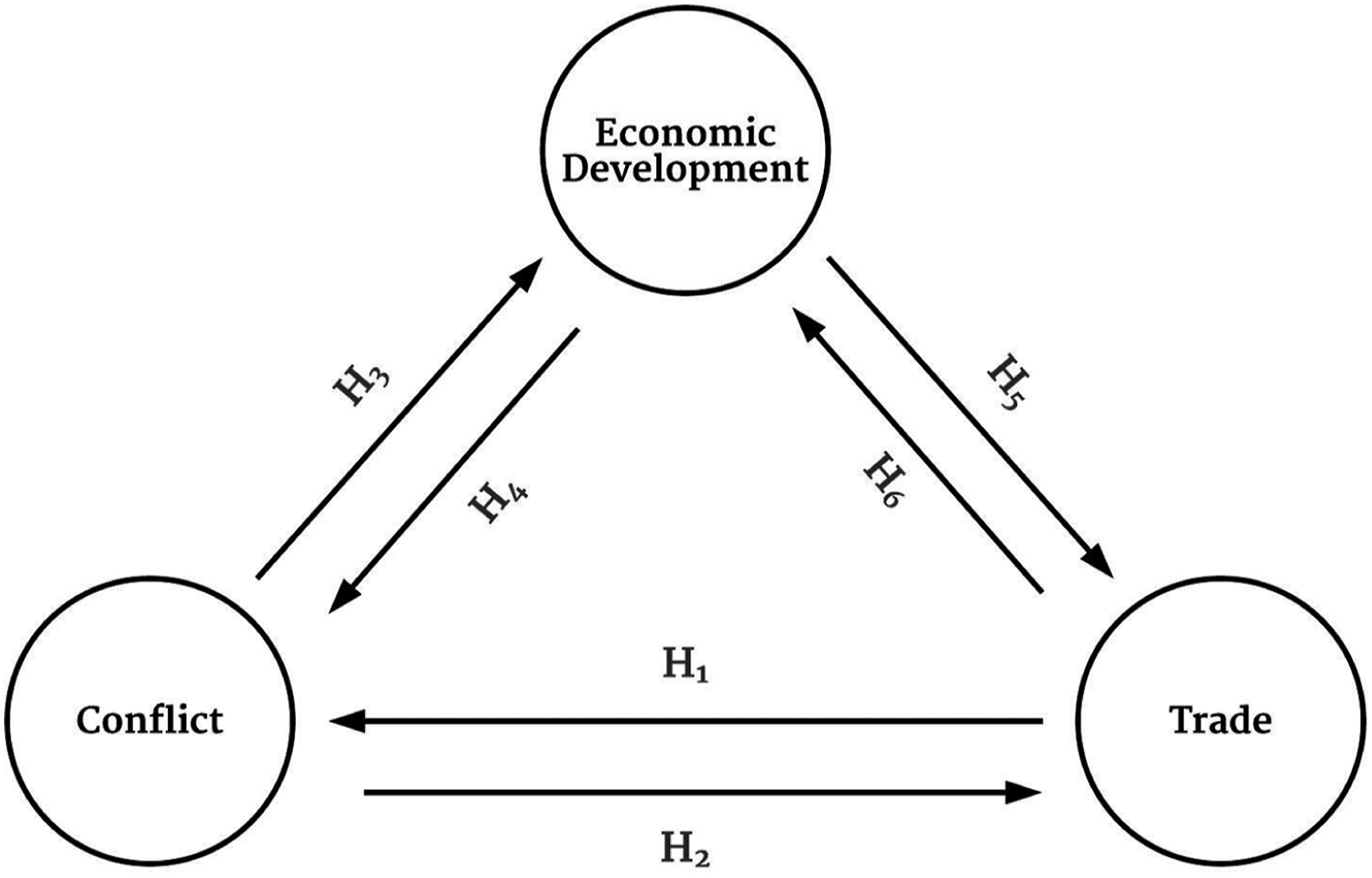
Interstate conflict is the primary outcome variable of interest in the present study. Accordingly, our SEM analysis will focus on the two hypothesized explanations for conflict: trade (H₁) and economic development (H₄). We will also examine the evidence for H₅ as we anticipate the indirect effect of development on conflict mediated by international trade. Of interest to regional scientists is the degree to which contiguity matters. Tobler famously quipped in his 1970 classic that “everything is related to everything else, but near things are more related than distant things” is the first law of geography. As it turns out, geographical proximity also engenders influence on interstate conflict. Accordingly, we will review the literature on the spatial aspect of militarized disputes. But first, we discuss one mechanism through which conflict affects the economy (H₃) as proposed by Kieran Donaghy.

Donaghy’s Model of Arms-Race Dynamics

Kieran Donaghy was trained at Cornell’s Graduate Field of Regional Science, and it was probably his interactions with Walter Isard at Cornell that motivated him to examine the effect of the Cold War on the American economy. His study, which appeared in Conflict Management and Peace Resolution (Donaghy 1995), was essentially an empirical inquiry of hypothesis H₃ in Figure 1 above. Of interest here is an equation in his continuous-time model describing how the United States military spending would respond to the perceived differences in military weapon stockpiles between the US and the Soviet Union:

DGMUS = g_{1} (ARMSOV - ARMUS) + g_{2} GMUS + g_{3} VN + g_{4} USPT

(1)

where DGMUS and GMUS are, respectively, the change in and the level of the US military government spending, ARMUS is the American stockpiles of military weapons, ARMSOV the corresponding Soviet stockpiles, VN the US expenditures on the Vietnam War, and USPT a measure of tension perceived by the Americans.

In Donaghy (1995), the arms race enters the national income identity equation where aggregate output depends on total government spending, including military expenditures. The parameter $g_{1}$ , in particular, represents the US government’s reaction to disparities in military capabilities. A positive difference between ARMSOV and ARMUS corresponds to a superior Soviets arsenal, which would motivate the US to increase its military expenditures. The positive change in the US military budget, DGMUS, would lead to an elevated level of US government spending, which affects the macroeconomy via rising aggregate demand and hence the stability of the American economy.

Reduced-form estimations based on data from 1961 to 1979 revealed robust results consistent with an earlier study using a longer time series (Donaghy 1993). The key finding is that none of the exogenous variables considered, including the Vietnam War costs and the perceived military threat of the USSR, had a measurable influence on the US military spending and stockpiles. The result provides an answer to Donaghy’s inquiry into the economic implications of arms races and international tension. Further, while reducing the US defense budget would have led to a non-trivial fall in real GDP, the contraction amounted only to about a 3.5 percent fall from the baseline output level. Donaghy (1995) concluded that the Cold War arms races “do not appear to have had much influence on economic developments.”

We report below our assessment of hypothesis H₃ based on a cross-country panel analysis. First, we review research that investigates our study’s primary hypotheses of interest: H₁, H₄, and H₅. We begin with the literature primarily by scholars of international relations examining H₁. In this literature, the empirical analyses rely on the available measures of the theoretical constructs, such as conflict, trade, and the economy. This paper uses real GDP as a proxy for economic development, which we also refer to as living standards when measured in per capita terms. Based on the living standards indicator, we will review studies examining the effect of the economy on conflict (H₄) and interstate commerce (H₅).

H₁: Trade affects Conflict

There is a vast literature on the relationship between economic interdependence and violent conflict. We think it is fair to say that international relations scholars tend to identify with one of two opposing views. Liberals contend that interdependence brings peace. Realists argue that interdependence brings conflict. According to the liberal proposition, commercial ties produce benefits that increase the opportunity costs of a dispute. These costs, therefore, serve as a deterrent to war. According to the realist theory, however, trade ties may compel a state to use force when it believes it is in danger of losing overseas access to raw materials or exports markets (Morelli and Sonno 2017). Thus, both liberalists and realists agree that trade affects conflict, but they disagree on the sign of the effect. Liberals believe that trade promotes peace realists believe in the opposite.

Polachek (1980) is an early empirical study that supports the liberal view. His main finding, which captures the spirit of the liberal view (Polachek 1980, 63), is that the doubling of trade between countries reduces interstate hostility by at least 15 percent. Subsequent liberalists, using a different method or an expanded dataset (e.g., Oneal and Russett 1997, 1999; Russett and Oneal 2001; Russett et al. 1998), sought to further demonstrate the pacifying effect of interdependence with evidence that more openness brings peace. Thus, the logistic regressions of Oneal and Russett (1997) show that a one-standard-deviation increase in economic openness reduced the probability by a significant margin that a state would engage in a militarized dispute. More recently and building on this literature, Chatagnier and Lim (2021) found that membership in the World Trade Organization also facilitates peace among WTO member countries.

In contrast, proponents of the realist view (e.g., Barbieri 1996; Beck et al. 1998; Reuveny and Kang 1998) argue that the effect of trade is not only much subtler but often brings crises as well. The primary source of disagreement is the differences in the measure of interstate commerce. We review the work of Barbieri (1996) to highlight the ambiguous nature of the relationship between trade and conflict. Barbieri (1996) constructed three measures, which she referred to as salience, symmetry, and interdependence, to address the effects of economic ties on conflict. Her findings are threefold. First, dyads that trade more extensively with each other (i.e., have more salient economic ties) were also more likely to enter into a conflict with each other. And while Barbieri did find that dyads with more equal reliance on each other (i.e., more symmetrical ties) were more likely to be at peace with each other, she also found that higher levels of interdependence (defined as the product of salience and symmetry) rendered dyads more prone to conflict with their trading partners. Barbieri (1996, 42) concluded that, in general, “extensive economic interdependence increases the likelihood that dyads engage in militarized dispute.” Following the same line of argument, more recently Petersen and Wen (2021) found that trade provokes armed conflict among states with greater military capabilities.

Liberalists and realists also disagree about the proper conception of trade. The liberalists Oneal and Russett (1997) argue that as the trade-to-GDP ratio represents the importance of trade relative to the size of the economy and it is the appropriate measure of openness. According to liberalists, the trade-to-GDP ratio captures the opportunity cost of a military dispute, and this discourages potential trading partners from doing business with a conflict state. In contrast, the liberalist Barbieri (1996) favors the share of imports/exports with its partners in the total trade as a measure of interdependence. Based on the trade share measure, Barbieri then constructed her salience, symmetry, and interdependence variables. Our SEM analysis compares the realists’ conflict model where imports/exports per capita are the explanatory variable to the liberalists’ model where imports/exports share in total trade is the explanatory variable.

Rarely does either camp (liberal or realist) of quantitative methodologists consider how an economy’s size affects the nature of the trade-conflict relationship. One reason is their research design focuses on dyadic relationships. In contrast, economic development is a concept that pertains to an individual state: economic development is a monadic phenomenon not a dyadic one.

H₄: Economic Development affects Conflict

The size of a nation’s economy has been identified as a critical factor affecting the relationship between interstate commerce and militarized conflict (Copeland 2014). Indeed, empirical studies suggest that the economy is a confounding factor that affects the pacifying influence of trade. Hegre (2000) found that the strength of the relationship between commercial ties and peace depends on economic development. Since aggregate output is correlated with trade (hypothesis H₅), statistical analyses that do not control for economic performance are vulnerable to omitted-variable bias. That is because any statistical association between imports/exports and violent disputes can be due to the direct effect of the former (hypothesis H₁ above) or to the indirect influence of the economy transmitted via trade. Thus, models seeking to establish the causal pathway from trade to conflict would need to control for the economic impact on both.

There is a literature strand that argues that rising living standards increase a state’s potential for war-making (Mansfield 1988). According to Doran (1983), this is because a prospering economy enables governments to direct scarce resources to arms procurement. Doran (1983) argues further that aggregate output is the single most important indicator of national power. The concept of power refers to the resources available for a polity to pursue its ambitions, which often include military dominance. Modelski and Thompson (1996) propose that economic development increases the demand for raw materials and new export markets, and these needs increase the possibility of confrontations. This mechanism is an extended version of the realist view that trade brings conflict; here, rising productivity creates surpluses, making a state more likely to fight other states to secure the market for its exports.

We refer to the positive association between output and conflict as evidence in support of the Kondratieff hypothesis, which posits that the most disastrous crises occur following a period of sustained economic expansion (Kondratieff 1935). The Kondratieff hypothesis is consistent with Doran’s (1983) argument that a growing state tends to spend more on the military. This expansion in military capabilities encourages the state to use amassed armed forces (Pollins 2008). We note that the direction of influence runs from the arsenal buildup via a growing economy to interstate conflict. In contrast, Donaghy (1995) asserts the opposite causation from the Cold War to the economy. The two pathways are not mutually exclusive: our SEM causal framework enables us to test both Kondratieff and Donaghy’s predictions simultaneously.

H₅: Economic Development affects Trade

Hypothesis H₅ asserts that more-developed countries are more likely to trade with the rest of the world. That countries that trade more tend to grow faster is a pattern of association that has been extensively studied (Dollar and Kraay 2003; Harrison 1996). Indeed, the theory of comparative advantage posits that economic openness enables countries to enjoy higher consumption and output levels than would have been possible without trade (Krugman and Obstfeld 2009). Causality in the comparative advantage literature, however, runs from openness to living standards, and not the other way around.

Markusen (2013) developed a theoretical model predicting more trade between nations with higher living standards. In his model, industrialized countries have a higher capacity to produce exports and higher income to consume imports than developing economies. Such prediction is consistent with the traditional gravity equation, which specifies that trade flows are proportional to per capita income levels (Anderson 1979). Econometric studies confirm that per capita GDP is a statistically-significant and sizable predictor of trade flows (Egger 2002). The nature of the relationship was well articulated by Frankel et al. (1998). They pointed out that, in addition to the size effect, more developed economies also tend to specialize more and therefore trade more. Accordingly, the present study examines the hypothesis of the positive impact of economic development on exports/imports.

Spatial Effects

Empirical studies have shown that wars are more likely to occur between nations with a common border (see, e.g., Senese 1996; Vasquez 1995). Both liberalists (e.g., Oneal and Russett 1997, 1999) and realists (e.g., Barbieri 1996; Beck et al. 1998) agree that border issues increase a state’s willingness to start a military confrontation. Very simply, contiguous states are more likely to fight each other because it is costlier to fight distant countries with conventional weapons. According to this train of thought, contiguity directly brings conflict.

At the same time, trade flows, also, are inversely related to geographical distance (Eaton and Kortum 2002; Tinbergen 1962). Closer countries incur lower transportation costs, making it easier to ship goods and services across borders. If trade brings conflict, as realists argued, proximity would also indirectly increase the propensity for states to quarrel through commercial ties. Barbieri (1996) found that interdependence and contiguity work in tandem to increase conflict. But if interdependence brings peace, as liberalists contended, proximity would mitigate conflict via the pacifying effect of trade. In this view, distance and interdependence interact to determine conflict intensity. Robst et al. (2007) show that interstate disputes fall when both trade and the distance increase by more than when only trade increases. We investigate in our SEM analysis whether trade intensifies or diminishes the conflict-inducing effect of geographic proximity.

The studies above focus not on trade spillovers into neighboring states and the chain of events that occur--but on the likelihood that a state will engage in military conflict through its trading activities. In the context of interstate trade, a spillover refers to an increase in country A’s trade activities that subsequently affects an adjacent country B. The ripple effect has been attributed to the network relations that transmit an exogenous shock within one economy (e.g., a productivity shock) to other economies in the network through interstate linkages (Chaney 2014). According to the liberal view, the possibility arises that Neighbor B interprets State A’s increased commercial ties as evidence of a peace-seeker. The interpretation encourages B to seek peace. According to the realist view, State B may interpret State A’s increased trade activities as an indicator of rising hostility, making B more combative and primed for a future conflict. In both cases, the result is the spillover of trade effects to neighboring countries. We explore trade in bordering states as the mechanism that pacifies (or ignites) conflict using a spatial SEM.

The Model

The triangular interrelationship between trade, conflict, and economic development (Figure 1) implies a system of equations with multiple outcome variables. Two alternative methods exist to draw causal inferences in a setting with interdependent variables. A structural equation modeling approach is one alternative. The other is the instrumental variables (IV) technique, which relies on an instrument Z to trace the effect of an endogenous variable X on the equation’s outcome variable Y. While it is usually implemented using two-stage least squares, the IV method boils down to the estimate of a single equation where Y is regressed against the Z-instrumented X (Angrist and Krueger 2001). Such a “reduced form” approach may yield a consistent estimate of the causal effect of X on Y, but it does not spell out the underlying generative mechanisms.

We develop an SEM in the endeavor to spell out the system of equations involving trade, disputes, and economic development. The estimation of an SEM is guided by the theoretical relationships among the variables that must be articulated before data are collected (Kline 2015, 10). In formal terms, specification is the process in structural equation modeling that describes causal connections using equations and identifies the right-hand-side variables in each equation (Kenny 1979). For our study, to specify is to translate H₁ and H₄ into equations describing the causal relationship between trade and conflict (H₁) and between the economy and conflict (H₄). Similarly, specification entails expressing H₅ in an equation to describe how development affects interstate commerce.

A search on the homepages of the Annals of Regional Science, Journal of Regional Science, Papers in Regional Science, and Regional Science and Urban Economics identified several SEM-based studies. For example, Van Oort et al. (2009) employs a latent-variable model to measure the spatial employment impact of the knowledge economy. Pagliara et al. (2021) develop an SEM to determine the causal effect of transportation infrastructure development on citizens’ trust in local government. Recent SEM works appearing in the International Regional Science Review cover topics that range from examining the determinants of city residential attractiveness (Kourtit et al. 2021), modeling sustainable tourism (Jiménez-Medina et al. 2021), modeling travel behavior (Gim 2016), and university impact on regional innovation activities (Mascarenhas et al. 2022).

A relatively new feature of structural equation modeling is the integration of graph theory for causal analyses (Elwert 2013). The result is the so-called causal diagram (CD), which represents the data generating processes using directed graphs (Pearl 2009). We take advantage of the CD’s ability to represent causal relationships using a non-parametric path model with unidirectional effects, consistent with the recursive nature of Donaghy’s (1995) model and the SEMs we consider in this review. We employ both CDs and equations in describing our SEM specifications below.

Every structural model considered in this paper includes two equations. The first represents the hypothesized effect of living standards on trade (i.e., H₅), while the second represents the claim that trade influences conflict propensities (i.e., H₁). We begin with the basic specification that considers only observable variables. Namely, the number of militarized disputes (nmids) a state participated in a particular year, per capita real GDP (RGDP/cap) as an operationalization of economic development, and per capita imports (imports/cap) as a measure of trade activities.⁴ If we also allow for the possibility for RGDP/cap to affect conflict directly (H₄), the model can be described using the CD in Figure 2:

Figure 2.

Basic specification in a causal diagram.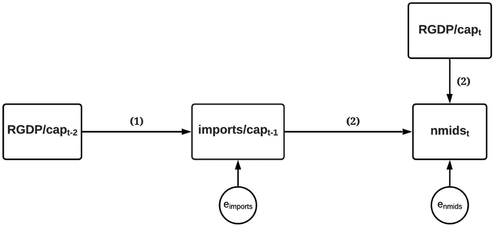

Every node on a CD represents an SEM variable, and every arrowhead represents a causal connection between an explanatory variable and an outcome variable. The effect must precede the outcome in the temporal sense for the former to be a candidate explanation of the latter. Thus, when the outcome variable appears with the t subscript, the explanatory variables would appear with the t-1 subscript. The numbers on the CD correspond to the equations where the paths appear, which will be discussed next. For now, we note that the relationship between living standards and imports is expected to be positive; nations with higher RGDP/cap are expected to import more to meet their consumption needs. The nature of the relationship between imports and interstate conflict is ambiguous; it is negative according to the liberalists but can be positive according to the realists.

A CD presents a natural way to show the dependencies because a structural model involves multiple equations with as many dependent variables. But the relationships embedded in an SEM can also be represented using the equivalent equations as follows:

{\frac{i m p o r t s}{c a p}}_{t - 1} = α_{0} + α_{1} {\frac{RGDP}{c a p}}_{t - 2} + e_{i m p o r t s},

(2)

{n m i d s}_{t} = β_{0} + β_{1} {\frac{i m p o r t s}{c a p}}_{t - 1} + β_{2} {\frac{RGDP}{c a p}}_{t - 1} + e_{n m i d s} .

(3)

Equation (2) describes the hypothetical relationship between living standards and trade, while equation (3) describes the relationship between trade and conflict. Thus, $α_{1}$ is expected to be positive, while the sign for $β_{1}$ is ambiguous: negative if the liberal view prevails but may be positive if the realist view holds.

The basic specification highlights two other features of structural equation modeling that are particularly pertinent for the present study. Unlike single-equation models, an SEM can identify the indirect channels of impact transmission. According to equations (2) and (3), trade has a double role as both an outcome and an explanatory variable; imports/cap is the outcome of RGDP/cap and the cause of conflict. Formally, the chain

RGDP / cap \overset{(2)}{\to} imports / cap \overset{(3)}{\to} nmids,

(4)

is an indirect pathway transmitting the effect of living standards on nmids via trade. In SEM terminology (Baron and Kenny 1986), imports/cap is an intervening variable mediating the relationship between an origin and a destination node. The magnitude of the indirect effect is defined as the multiplication of the coefficients on the individual paths (Kline 2015). Thus, the impact of living standards on conflict mediated by trade is the product

α_{1}

∙

β_{1}

; the effect of a change in RGDP/cap on imports/cap times the effect of a change in imports/cap on nmids.

Second, an SEM allows the direct effect of X on Y to be estimated while controlling for the indirect pathways (Bollen and Stine 1990). Thus, since H₅ states that economic development causes trade and H₁ states that trade, in turn, causes conflict, it makes sense to control for the intervening variable if we are to measure the direct effect of development on conflict. In our SEM, the coefficient $β_{2}$ in equation (2) represents the direct influence of a change in RGDP/cap on nmids, controlling for the indirect effect of the former mediated by imports/cap. The path decomposition of the total impact into indirect and direct effects enables the various generative mechanisms that induce a change in the outcome variable to be identified.

Estimation of the simple SEM would yield the gross effects of per capita output on imports and trade on conflict. To address the possibility of omitted variable bias, we would need to extend the specification with additional controls. The path diagram in Figure 3 considers other variables that could also explain the variations in trade and conflict.

Figure 3.

Extended specification in a path diagram.

The extended specification for per capita imports controls for a state’s workforce (emp), iron and steel production (irst), and primary energy consumption (pec). At the same time, the conflict model now controls for membership in a military alliance (allied), the degree to which the state favors democracy (democ), population size (pop), and the number of military personnel (milper). We also assert that the incidents of militarized conflict (nmids) are influenced by the state’s military expenditures, as Donaghy (1995) did in his arms race model.

We can also describe the extended SEM using equations as follows:

{\frac{imports}{cap}}_{t - 1} = α_{0}^{'} + α_{1}^{'} {\frac{RGDP}{cap}}_{t - 2} + α_{2}^{'} {emp}_{t - 2} + α_{3}^{'} {irst}_{t - 2} + α_{4}^{'} {pec}_{t - 2} + e_{imports},

(5)

{nmids}_{t} = β_{0}^{'} + β_{1}^{'} {\frac{imports}{cap}}_{t - 1} + β_{2}^{'} {\frac{RGDP}{cap}}_{t - 1} + β_{3}^{'} {allied}_{t - 1} + β_{4}^{'} {democ}_{t - 1} + β_{5}^{'} {pop}_{t - 1} + β_{6}^{'} {milper}_{t - 1} + β_{7}^{'} {milex}_{t - 1} + e_{nmids} .

(6)

Countries with a larger workforce are expected to import less through their ability to produce more output for domestic consumption. Hence, we anticipate a negative sign for the employment coefficient $α_{2}^{'}$ . Similarly, we expect the coefficients on iron and steel, $α_{3}^{'}$ , and energy consumption, $α_{4}^{'}$ , to be negative in the imports model. Following the international relations literature (e.g., Oren 1990), we expect alliance members to engage in more conflict because of the obligations to the alliance, which can be a mutual defense pact, a treaty, or an entente. Likewise, states that spend more on military purchases and have a larger armed force are expected to participate in more disputes (Fordham 2004). If that is the case, $β_{3}^{'}$ , $β_{6}^{'}$ , and $β_{7}^{'}$ should enter with a positive sign. In contrast, multiple studies have demonstrated the pacifying effect of democracy on conflict (e.g., Altman et al. 2021). The coefficient $β_{4}^{'}$ in equation (6) thus has an expected negative sign.

The literature review also discusses the importance of contiguity in explaining the variations in conflict incidents. Accordingly, we predict countries with more adjacent neighbors to engage in more militarized confrontations. Despite the robust statistical evidence, few studies shed light on the mechanism that explains why bordering neighbors are more likely to fight one another. As Vasquez (1995) put it, the reason for this is not well understood and is an area in great need of multidisciplinary research. We believe that Regional Science as an interdisciplinary field can offer an insight into the role of geography in the onset of an interstate dispute.

Boulding (1962) offers a theoretical exploration of the association between proximity and interstate disputes. His theory of conflict has the flavor of Tobler’s (1970) first law of geography. According to Boulding (1962), the distance between (potential) enemies is similar to the impact of transportation costs on competing firms. In particular, diminishing distance makes it more likely for a country to attack another country in the same way that falling transportation costs make it more likely for a firm to ruin its rival. Just as predatory pricing is less costly in a price war when shipping costs are lower, says Boulding (1962), proximity makes it easier to project military force to an immediate neighbor.

We explore the mechanisms of conflict transmission where the changing characteristics of the neighbors affect a state’s decision to engage in a conflict. For instance, neighbor A’s decision to enter a military alliance that state B is also a member of would make it imperative for the latter to join a confrontation when the former is attacked by another state C. Alternatively, if state B joins an alliance that state A considers hostile, then state A is now more likely to attack state B who is now perceived to be a friend of an enemy.

Yet another possibility is an increase in state A’s military expenditures that its neighbor B considers a security threat. A conflict could be imminent in the middle of an arms race if state A’s stockpiling of weapons signals that A is priming for an invasion into B’s territory (Donaghy 1995). At the same time, a pacifying effect is also possible when state A’s increasing trade activities are interpreted as evidence of state A’s willingness to integrate into the global economy.

A spatial interaction occurs when a state’s characteristics influence a neighbor’s decision to enter a conflict. When the influence does not induce endogenous feedback, we have the phenomenon of local spillovers (LeSage 2014). Spillovers occur, for example, when a state A considers the growing economic prosperity of neighbor B as a threat that motivates A to strike first. Such a conflict would be consistent with the Kondratieff hypothesis, which posits that a prospering state is more likely to participate in a dispute. Therefore, a local spillover specification means economic development in A influencing its neighbor B’s decision to enter a militarized conflict. Chaney’s (2014) trade network hypothesis is another spillover mechanism whereby increased openness in A has an impact that travels across the borders to a neighboring state B.

The local spillover specification is consistent with the so-called spatial lag of X (SLX) model:

y = X β + W X δ + e,

(7)

where W is a spatial-weight matrix multiplied by the explanatory variables X to yield the spatial lag vector, WX. Of theoretical interest here is the vector

δ

, which captures the effect on one state’s outcome variable, y, of changes in the determinants of all the neighboring states. Thus, the product

W X δ

represents the weighted average of changes occurring in all bordering neighbors that spill over into a given location. For example, based on the specification in equation (2), the corresponding SLX model for conflict is as follows:

{nmids}_{t} = β_{0} + β_{1}^{s} {\frac{imports}{cap}}_{t - 1} + β_{2}^{s} {\frac{RGDP}{cap}}_{t - 1} + W X_{M} δ_{M} + W X_{R G D P} δ_{RGDP} + e_{nmids},

(8)

where

β_{1}^{s}

and

β_{2}^{s}

are the coefficients of own state’s per capita imports and RGDP, respectively,

δ_{M}

is a spillover coefficient capturing the indirect (i.e., other-region) effects of trade activities in the neighboring states, X_M, and

δ_{RGDP}

represents the indirect effects of economic development in the same neighbors, X_RGDP. A negative

δ_{M}

would corroborate the spatial version of the liberal view, while a positive one would be consistent with that of the realist view. At the same time, a positive

δ_{RGDP}

would be taken as evidence supporting the Kondratieff hypothesis.

The next section presents the data used to test the various hypotheses embedded in the different specifications of the SEM, including the local spillover specification.

Data

Conflict Data

The source of conflict data is the Correlates of War (COW) project, which has aimed since its inception to systematically collect information about international conflict (Gochman and Maoz 1984). Militarized interstate disputes (MIDs) are incidents that range in intensity from threats to use armed force to actual combat. Such a confrontation would qualify as MID if it did not escalate into a full-scale war. The MID data collection is available through the COW project website. The present study utilizes version 4.3 (Palmer et al. 2015), covering militarized disputes among 192 countries between 1816 and 2010.

The qualifier “interstate” limits the universe of conflicts to interactions among recognized nations and excludes non-state actors. Thus, an MID arises when a state’s threat or use of military force is explicitly directed toward another state (Jones et al. 1996). MID 4.3 records information about 2315 such events between 1816 and 2010. An example was the 2008 conflict that began when a platoon of Indonesian soldiers raided a border village in Papua New Guinea to search for a purportedly missing Indonesian officer. Another dispute was evident from the 2010 flyover of a Chinese naval helicopter around a Japanese destroyer near Okinawa. Yet another example occurred when North Korean ships briefly violated South Korean waters in 2008. All these incursions involved either the threat, display, or use of force but were short of the sustained combat that characterizes war.

Our analysis' primary dependent variable of interest is the number of disputes (nmids) that a state participated in a particular year. As Figure 4 shows, the overall frequency of MIDs generally was trending upwards over the period covered by the COW dataset. The long-run trend suggests that not only conflict has remained omnipresent since at least the early part of the 19th century, but the frequency of incidents has also been increasing over time.

Figure 4.

Frequency of interstate militarized disputes, 1816–2010.

Trade and National Income Data

Trade and living standards are the main explanatory variables in the model for conflict (Equations (3), (5), and (7)). The Correlates of War project keeps track of export and import activities for over 200 states between 1870 and 2014. The primary source of the post-WWII data is the IMF’s Direction of Trade Statistics, while the pre-WWII figures are from Barbieri (2002). While exports and balance of payments data are available, the estimation results reported below employ per capita imports to gauge trade activities. All trade statistics are in millions of US dollars.

The Penn World Table (PWT) version 10.0 is the source of national income and output data for 183 countries between 1950 and 2019 (Feenstra et al. 2015). The variables we extracted from the PWT database are:

Nominal gross domestic product (GDP).

Real GDP at constant 2017 national prices (in millions of 2017 US dollars).

Total population (in millions of people).

The national workforce size (number of persons engaged in production).

We use population data (pop) as a control variable and the denominator of per capita output and trade. Likewise, we utilize employment data (emp) as an explanatory variable and the denominator of per-worker output.

Contiguity and Other Variables

The variable direct contiguity (contig) counts the number of adjacent neighbors directly contiguous to a state. The COW website describes five available categories of contiguity, namely, one for land contiguity and four categories based on 12, 24, 150, and 400 miles separation, respectively, by water. Land contiguity is the interface between the homeland borders of two states that occurs through a land boundary or a river. In contrast, the water boundaries are based on whether a straight line can be drawn between the edge of one state, across a body of water, and its neighbor’s borders, uninterrupted by a third state (Stinnett et al. 2002).

In the most recent MID dataset (version 5.0), conflicts between contiguous countries include the border tension between Indonesia and Malaysia that emerged in 2014 after Malaysia began the construction of a lighthouse in waters claimed by both countries. The Southeast Asian neighbors dispatched their naval warships to the disputed maritime borders. In the same year, six Egyptian soldiers were killed when Israel bombed the Egyptian border with Palestine. In another incident, Ukraine began fortifying the border with Russia following Russia’s annexation of Crimea in 2014. While the show of force stopped short of a full-scale war then, both Ukrainian and Russian troops crossed the border multiple times that year.

Power is the central concept underlying the National Material Capabilities dataset, which keeps track of annual military expenditures (milex), military personnel (milper), primary energy consumption (pec), and iron and steel production (irst). These and other indicators form the basis of the composite index of national capability (Singer et al. 1972). The present study employs version 6.0 of the dataset, covering the 1816–2016 period.

A state is identified as a member of an international military alliance if it is committed to a formal treaty ratified by two or more nations (Gibler 2008). The Correlates of War database recognizes four different categories of such alliances. A defense pact is the highest level of military commitment, binding alliance members to provide military support to a member attacked by a third party. A lower commitment level would be categorized as either neutrality or non-aggression, requiring members to remain neutral or to not use force in case of conflict with another member of the alliance. The lowest level of commitment is an entente, which requires members to consult in times of crisis but without additional obligations. Following Barbieri (2002), we calculated the total number of alliances (allied) that a state belonged to using version 4.1 of the dataset.

The democracy index (democ) is an additive eleven-point scale (0–10) coded based on the competitiveness of political participation. Thus, countries where political participation is unrestricted, open, and fully competitive score highly in the index. The source data is the Polity5 Project database posted on the Center for Systemic Peace website. The Polity5 dataset covers the 1800–2018 period.

The resulting intersection of the various datasets considered in this study covers 168 countries for the 1950–2010 period. Table 1 lists the variables considered in the SEM analysis and their definitions. The summary statistics for these variables and their pairwise correlations are in Table 2.

Table 1.

List of Variables, Definitions, and Data Sources.

Variable	Definition	Data Source
Nmids	Number of militarized disputes	COW project
imports/cap	Per capita imports (million US$)	COW project
RGDP/cap	Per capita real GDP at 2017 prices	PWT
Contig	Number of contiguous neighbors	COW project
pop	Total population (million people)	PWT
emp	Workforce size (workers)	PWT
milex	Military expenditures	NMC dataset
milper	Number of military personnels	NMC dataset
irst	Iron & steel production	NMC dataset
pec	Primary energy consumption	NMC dataset
democ	Democracy index	Polity5 project

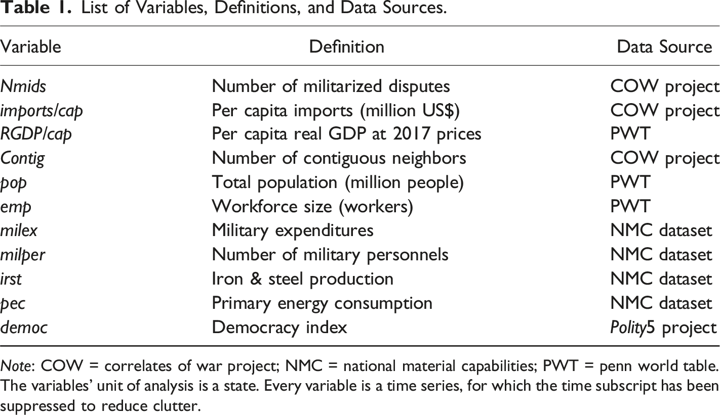
Note: COW = correlates of war project; NMC = national material capabilities; PWT = penn world table.

The variables' unit of analysis is a state. Every variable is a time series, for which the time subscript has been suppressed to reduce clutter.

Table 2.

Descriptive Statistics.

	(1)	(2)	(3)	(4)	(5)	(6)	(7)	(8)	(9)	(10)	(11)
Unique bivariate correlation coefficients
(1) nmids	1
(2) imports/cap	−0.0472	1
(3) RGDP/cap	−0.00980	0.293	1
(4) contig	0.262	−0.0553	0.0611	1
(5) pop	0.276	−0.0384	−0.0728	0.383	1
(6) emp	0.264	−0.0317	−0.0568	0.374	0.984	1
(7) milex	0.266	0.0163	0.180	0.105	0.243	0.248	1
(8) milper	0.436	−0.0449	−0.0187	0.387	0.771	0.761	0.393	1
(9) irst	0.241	0.00276	0.0876	0.249	0.559	0.624	0.394	0.509	1
(10) pec	0.358	−0.00256	0.142	0.251	0.585	0.621	0.759	0.668	0.819	1
(11) democ	−0.0173	0.147	0.239	−0.0286	−0.00633	−0.0130	0.131	0.00542	0.108	0.125	1
Univariate descriptive statistics
Mean	0.373	2663.462	13434.13	5.441	33.034	33.034	14.793	14.793	4650715	161.429	161.429
Std deviation	0.895	12707.89	18511	3.413	118.584	118.584	58.859	58.859	28300000	472.942	472.942
Min.	0	0.058	246.857	0	0.040	0.040	0.015	0.015	0	0	0
Max.	25	362437.3	204345.4	29	1399.454	1399.454	794.6456	794.6456	694000000	5800	5800
No. observations	9023	8037	8485	9023	8485	8485	7911	7911	7948	8255	8255

Results

Table 3 reports the estimated coefficients and the relevant statistics for four models this study considers. Consistent with the gravity model literature and in support of H₅, estimates of the basic specification (Figure 2) show that countries with higher per capita output also tend to import more. Specifically, every standard deviation increase in log RGDP per capita is associated with a 0.798 increase in standardized per capita imports. Since the standard deviation of log RGDP per capita (lagged twice) is 1.230, the estimate means that each one-percent increase in RGDP per capita is associated with a 0.65 standard deviation increase in imports per capita. Given the standard deviation of imports per capita (lagged once) of 2.032 US dollars, the increase is equivalent to US$1.32 of per capita imports for every one-percent increase in per capita RGDP.

Table 3.

SEM Estimation Results.

	(1)	(2)	(3)	(4)
LHS: ${i m p o r t s / c a p}_{t - 1}$
$\log {R G D P / c a p}_{t - 2}$	0.799*** (121.21)	0.732*** (83.44)	0.642*** (70.99)	0.627*** (69.61)
${\log e m p}_{t - 2}$		−0.183*** (−16.41)	−0.160*** (−13.51)	−0.202*** (−16.52)
${i r s t}_{t - 2}$		0.0401** (3.22)	0.0116 (0.76)	0.000162 (0.01)
${p e c}_{t - 2}$		0.0141 (1.13)	0.120*** (4.98)	0.138*** (5.79)
${d e m o c}_{t - 2}$			0.0448*** (21.80)	0.0471*** (23.13)
${m i l e x}_{t - 2}$			−0.0147 (−1.04)	−0.0133 (−0.95)
${m i l p e r}_{t - 2}$			−0.000343*** (−12.88)	−0.000399*** (−14.96)
${c o n t i g}_{t - 2}$				0.0307*** (11.74)
Constant	0.00377 (0.57)	−0.0201* (−2.34)	−0.164*** (−12.84)	−0.345*** (−17.33)
LHS: $n m i d s$
${i m p o r t s / c a p}_{t - 1}$	−0.258*** (−14.98)	−0.0980*** (−4.58)	−0.101*** (−4.62)	−0.112*** (−5.12)
$\log {R G D P / c a p}_{t - 1}$	0.200*** (11.82)	0.0454* (2.32)	0.0462* (2.33)	0.0492* (2.48)
${a l l i e d}_{t - 1}$		0.0635*** (10.38)	0.0600*** (9.63)	0.0554*** (8.83)
${m i l p e r}_{t - 1}$		0.000746*** (25.40)	0.000698*** (19.00)	0.000639*** (16.68)
${m i l e x}_{t - 1}$		0.0686***(6.12)	0.0493** (3.21)	0.0567*** (3.69)
${d e m o c}_{t - 1}$		−0.000444 (−0.14)	−0.00107 (−0.34)	−0.000412 (−0.13)
${p e c}_{t - 1}$			0.000000122 (1.94)	0.000000122 (1.94)
${c o n t i g}_{t - 1}$				0.0203*** (5.27)
Constant	0.372*** (37.09)	0.153*** (6.59)	0.158*** (6.77)	0.0502 (1.61)
N	7722	4745	4645	4645

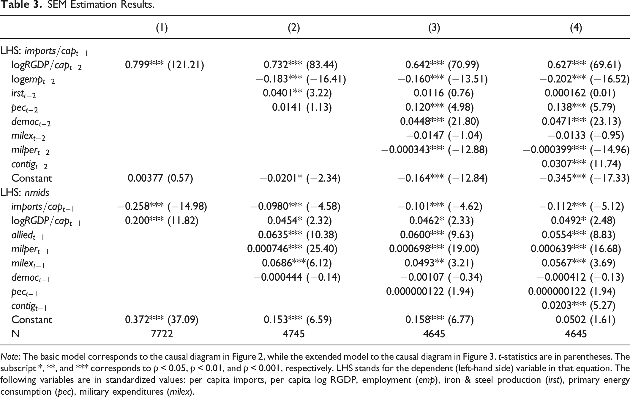
Note: The basic model corresponds to the causal diagram in Figure 2, while the extended model to the causal diagram in Figure 3. t-statistics are in parentheses. The subscript *, **, and *** corresponds to p < 0.05, p < 0.01, and p < 0.001, respectively. LHS stands for the dependent (left-hand side) variable in that equation. The following variables are in standardized values: per capita imports, per capita log RGDP, employment (emp), iron & steel production (irst), primary energy consumption (pec), military expenditures (milex).

In the equation for conflict, the negative coefficient on imports per capita lends credence to the neoliberal hypothesis. The coefficient indicates that one standard-deviation increase in imports per capita reduces the number of conflicts a state engaged in by one-fourth of an incident. At the same time, an increase in per capita output appears to be the impetus that led to a higher number of conflict participations. The estimated coefficient suggests the number of disputes a country is engaged in would increase by 0.2 incidents for every additional standard deviation increase in log RGDP per capita. All these estimates are statistically significant at the one-percent level in support of H₁ and H₄.

The estimated coefficients in the basic specification can be thought of as estimates of the gross effects. In contrast, the extended specification (Figure 3) controls for several economic and political characteristics in both the conflict and trade equations. The second column of Table 3 shows that the estimated influence of per capita output on per capita imports remains positive and significant at the one-percent level in support of H₅. Similarly, the pacifying effect of trade on conflict remains robust, supporting H₁ with a p-value <0.001.

The signs for the control variables also appear reasonable. In the trade equation, a larger workforce (emp) is associated with lower imports, presumably because more workers represent a greater self-sufficiency capacity. On the other hand, a higher level of iron and steel production (irst) leads to more imports, likely because such production requires inputs only available via the world markets. In the conflict equation, being a member of a military alliance (allied) and a buildup of military personnel (milper) are associated with greater involvement in conflicts. Likewise, a higher level of military expenditures (milex) corresponds to an increase in the number of disputes a state is involved in.

The full specification considers even more control variables in the trade and conflict equations to improve the model’s fit to the data. The third column of Table 3 reports that the positive effect of the economy on imports remains robust, supporting H₅ with a p-value <0.001. Likewise, dependencies on the rest of the world continue to have a mitigating effect on conflict. Specifically, a one standard-deviation increase in per capita imports, on average, reduces the conflict-participation rate by one-tenth of a dispute. The pacifying effect of trade is also statistically significant at the 1-percent level, providing H₁ with empirical support.

The fit statistics indicate the model’s excellent ability to reproduce variations in the dataset (i.e., the empirical variance-covariance matrix). The root-mean-squared error of approximation (RMSEA), comparative fit index (CFI), the Tucker-Lewis index (TLI), and standardized root mean squared residual (SRMR) all met the cut-off values for a good fit by a significant margin. This finding implies that the null hypothesis, which states that the overidentified SEM (with 13 degrees of freedom) is not consistent with the data, can be rejected.⁵

We consider next SEM’s ability to measure indirect effects, which refer to the influence of a cause on an outcome mediated by an intervening variable. Specifically, the pathway $RGDP / cap \overset{(2)}{\to} imports / cap \overset{(3)}{\to} nmids$ in equation (4) is an indirect mechanism where living standards affect conflict through trade. The estimated indirect impact in the full specification is the product $α_{1}$ ∙ $β_{1}$ , which results in a reduction of 0.06 dispute incidents for every standard deviation increase in log per capita GDP. Thus, economic development has an indirect pacifying effect, which contrasts with the direct impact contributing to a higher frequency of disputes (H₄). The opposite sign is due to the multiplication of the positive influence of RGDP/cap_t-2 on imports/cap_t-1 ( $α_{1}$ ) and the pacifying effect of the latter ( $β_{1}$ ). Economic development leads to more trade (H₅), which reduces the conflict participation rate (H₁). The pacifying indirect impact of living standards is statistically significant (p-value <0.001) with a magnitude comparable to the conflict-inducing direct effect of 0.05 incidents for every standard deviation increase in log per capita GDP. Other notable indirect channels include the paths from energy consumption (pec) and democracy index (democ), neither of which has a statistically significant direct effect on conflict. However, the indirect effects via trade are both peace-inducing and statistically significant at the 0.1-percent.

Of interest is how spatial proximity affects the volume of trade and conflict incidents. The estimated results (fourth column of Table 3) provide empirical support to Tobler’s first law of geography. In the trade equation, every additional contiguous neighbor (contig) is associated with an increase in imports per capita by 0.031 standard deviations. Bordering states are also more likely to fight each other. The coefficient on contig in the conflict equation suggests that every additional contiguous neighbor, on average, increases the conflict participation rate by 0.02 disputes. At the same time, the positive effect of living standards on imports (H₅) and the pacifying influence of trade on conflict (H₁) remain robust with a p-value <0.0001. The impact of living standards and globalization thus persist after controlling for border contiguity effects. Less clear, however, is how proximity matters in the two causal processes.

Accordingly, we explore next the mechanisms through which proximity influences trade and conflict. Specifically, we consider the SLX models to control for possible local spillover effects (equations (7) and (8)). The SLX models employ a row-standardized spatial-weight matrix, W, to generate the spatial lag variables. In our analysis, the W-matrix assumes the so-called queen criterion; neighbors are defined as states sharing at least one common border with the focal nation. The spatial weight matrix, W, for the countries of the world as of 2008 was generated from the shape file provided by thematicmapping.org.⁶

As the causal diagram in Figure 5 shows, the SLX model of conflict includes the spatial lag of militarized disputes, per capita imports, per capita log RGDP, population size, and the democracy index. At the same time, the SLX model of trade includes the spatial lag of per capita log RGDP, log employment, iron and steel production (irst), primary energy consumption (pec), and democ. Since the complete time series going back to 1950 (the first year GDP data are available in the Penn World Table) is incomplete for many countries, the following report is based on the subset of 146 countries for the 40 years between 1975 and 2014.

Figure 5.

The SLX model in a causal diagram.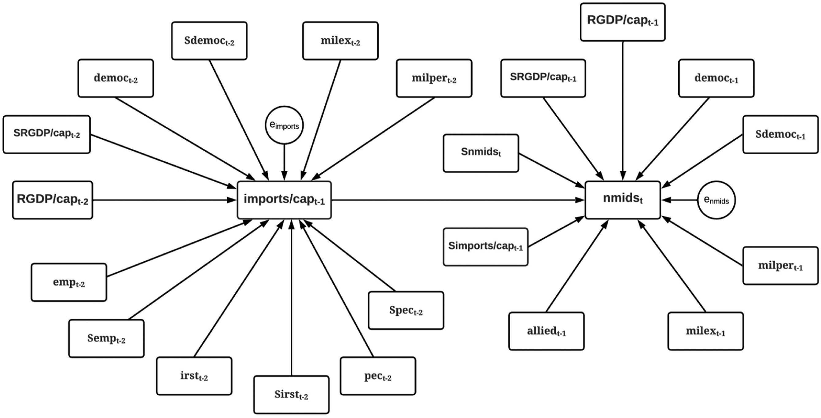

Results from the SLX model for conflict indicate that the pacifying effect of trade (H₁) remains robust. The estimated coefficient suggests that militarized disputes would be reduced by 0.1574 incidents for every standard deviation increase in per capita imports. However, there is no evidence that trade exerts a local spillover effect on conflict across the border. The estimated coefficient on the spatial lag of imports/cap is not statistically different from zero. Thus, the result rejects the network hypothesis (Chaney 2014), which posits the spillover effect of trade on neighboring countries. Nevertheless, the spatial model yields two additional insights.

First, proximity to neighbors with a higher democracy-index score leads to fewer conflicts. The coefficient on the spatial lag of democ is negative with a p-value <0.01. In contrast, the coefficient on own-democracy level is positive and statistically significant at the 1-percent, suggesting that democracies are more likely to participate in a dispute. The two results combined indicate that while democracies are vulnerable to attacks, vulnerability is lessened in the presence of neighboring democracies. Simply put, democracies do not attack each other.

Second, the coefficient on the spatial lag of nmids is positive with a p-value <0.05. That is, neighboring disputes heighten the degree of a nation’s participation in militarized conflicts. Since nmids itself is the dependent variable in the conflict equation, the result suggests a spatial autoregressive (SAR) process where dispute frequency in one location increases because of conflict at neighboring locations (Beck et al. 2006; Iqbal & Starr 2008). The full adjustment for spatial autocorrelations in an SEM requires an algorithm beyond the scope of this study. Nevertheless, the coefficient on lag nmids can be taken as a proxy of the first-round effect of disputes in neighboring states.

The final hypothesis we address is H₃, which asserts that conflict affects national economic performance. In his Arms Race Dynamics and Economic Stability, Donaghy (1995) concluded that the Cold War had a discernible but small impact on the US economy. Donaghy’s econometric model is, of course, a single-economy model of the United States. Our SEM allows us to examine the effect of militarized conflict on economic development in a multi-country panel setting. Specifically, we estimate an SEM augmented with a simple model of per capita RGDP. The model of economic development specifies militarized conflict (nmids), per capita total trade (ttrade/cap), and years of schooling (sch) as the explanatory variables:

\frac{RGDP}{cap} = f (nmids, \frac{ttrade}{cap}, sch) + e_{RGDP / cap}

where total trade is defined as the sum of exports and imports, education data (including years of schooling) are from Barro and Lee (2013), and

e_{RGDP / cap}

is the residual term. The model thus specifies a contemporaneous relationship between economic development and interstate disputes. As expected, the estimated effects of trade and education on living standards are positive and statistically significant at the 1-percent.⁷ However, the impact of conflict is not statistically different from zero. Consistent with Donaghy (1995), we found no evidence to support the claim that conflict disrupts economic stability (H₃). More work would certainly be warranted to address the identification challenges associated with such a simple model.

Discussion and Concluding Remarks

This study examines the role of economic interdependence and aggregate output in militarized disputes within the framework of structural equation modeling. The SEM estimations employ the Correlates of War data for 168 countries spanning the 1950–2010 period. We focus on three hypotheses, namely, that commercial ties affect conflict incidents (H₁) and that per capita output contributes to the frequency of such incidents (H₄) and the extent of trade activities (H₅). We pay tribute to Kieran Donaghy’s contribution to Peace Science in our exploration of the economic consequences of interstate disputes (H₃). The analysis considers alternative specifications to test the hypotheses using a system-of-equations approach.

Consistent with the liberal proposition, the pacifying effect of trade appears robust across different SEM specifications. The full specification is a comprehensive model that controls for standard explanatory variables in the peace science literature. The estimation results reported in the third column of Table 2 show that one standard-deviation increase in per capita imports, on average, reduces the conflict participation rate by 10 percent. Given the standard deviation of per capita imports (lagged once) of US$2.032, the increase is equivalent to 5 percent fewer militarized disputes for every dollar increase in per capita imports.

The results also reveal that trade is an important intervening variable between import determinants and interstate disputes. Specifically, the indirect influences of the economy, energy consumption, and democracy on conflict through imports are all statistically significant at the 0.1-percent level. These effects have a negative sign, suggesting that the second-order impact reduces conflict incidents. Furthermore, the magnitude is comparable to the direct effect, indicating that the indirect mechanism is as important as the first-order mechanism. Trade, therefore, is a mediator that transforms the conflict-inducing effect of the economy into a pacifying force on militarized disputes. The following discusses the implications of the findings for Kieran Donaghy’s broader body of work.

In Worlds Lost and Found: Regional Science Contributions in Support of Collective Decision-Making for Collective Action, Donaghy (2021) argues that there are theoretical and methodological advances in regional science that could help policy practitioners address the challenges of an increasingly complex world. Many of those advances remain “worlds lost,” waiting for regional planners to discover and use in their management of change. One such contribution is by Isard and Lewis (1984), who propose the use of subjunctive reasoning in policy analysis. Defined as reasoning about counterfactual scenarios that might have been true under different conditions, subjunctive thinking is particularly appropriate in the face of considerable uncertainty and imperfect foresight.

According to Isard and Lewis (1984), the subjunctive approach helps us understand causal relationships embedded in complex dynamic spatial systems. Donaghy (2021) argues that such an understanding of the causal mechanism at work in the social world is key to identifying the appropriate collective action (i.e., plan or policy) to combat socioeconomic problems with a spatial dimension. He cautions, however, against the indiscriminate use of random experimentation (Duflo et al. 2007), which detects mean differences between two groups but only in a highly-artificial setup where a single exogenous variable is changed in the so-called treatment group to measure causal effects. Randomizing a policy instrument is ill-suited for analyzing counterfactual scenarios when the policy intervention cannot be randomized (Barrett and Carter 2010). Randomization is not an option, for example, when an infrastructure facility is necessarily placed in regions that need it the most. Indeed, in the context of our research, it is virtually impossible to randomize interstate conflict or trade. If regional scientists are genuinely interested in answers to “what-if” questions about policies, Donaghy (2021) says what we may need (or should use) instead is the model-based approach to causal inferences with careful attention to the mechanisms of change.

Structural equation modeling is a model-centered approach to evaluating theoretical mechanisms against the available data. Indeed, since its inception, structural equation modeling has focused on identifying the causal processes responsible for the variations in the outcome variables (Grace et al. 2012). The term “system of equations” can be attributed to Trygve Haavelmo (1943). The econometrician was an early proponent of structural equations to describe causal structures instead of correlational relationships.⁸ According to Haavelmo, a system of equations is truly structural if every specified coefficient can be legitimately given a causal interpretation.

Structural models are the appropriate platform for scenario analyses, as Judea Pearl (2012) articulated most recently. The philosopher of computer science describes a counterfactual as “Y would be y had X been x in situation U = u.” In broad terms, a counterfactual is a probabilistic statement about what might have or could have happened under a condition different from the observed reality. According to Pearl (2012), the key here is to interpret “had X been x” as a counterfactual where mother nature assigns X a value different from the actual observed value, say x′ ≠ x. Such interpretation is appropriate for our study where no militarized conflict case can be tested twice, i.e., with and without the treatment of interstate trade, as would be required by an experimental design. Further, SEM can uncover counterfactual content when X itself is a dependent variable in some other equations, i.e., an interconnected system of equations.

Donaghy’s (1995) continuous-time econometrics model is, of course, a multi-equations simulation platform. Unlike a vector autoregression, his dynamic model expresses causal (i.e., structural) macroeconomic relationships where the arms race between the US and the Soviet influences output via military expenditures, a component of aggregate demand. Donaghy (1995) offers an important insight from the use of his model to simulate a counterfactual. If (a) the American perceived threat of the USSR and (b) the Soviet perceived threat of the US were simultaneously reduced to accompany lower military expenditures, the US would have experienced a much larger contraction of aggregate output. Since the US did not undergo such a dramatic fall in real GDP, the counterfactual simulation reveals that the Keynesian fiscal policy in place then had a stabilizing influence on the economic system. To the best of our knowledge, Donaghy’s simulation framework has not been applied to examine the implications of later conflicts (i.e., events more recent than the Cold War), such as the Gulf War, the US War in Afghanistan, or the US-China Trade War, for the American economy. A world lost indeed.

This review does not consider the relationship between militarized disputes and disaggregated trade. The literature has stressed this before (Reuveny and Kang 1998) and could be the subject of future research. In addition, previously-occupied regions can become independent. Moreover, nations can merge, and a country can disappear when annexed by another state. Future research could also address territorial changes using spatial weight matrices that reflect changes in countries and borders over time. The effect of conflict on trade (H₂) and trade on economic development (H₆) are two unexplored channels of impact transmission in the triangle of interdependence. At the same time, we consider only a single development indicator in this study--per capita output--and only one operationalization of interdependence in this study--interstate commerce. A work in progress will address this study’s limitations.

Footnotes

Declaration of Conflicting Interests

The author(s) declared no potential conflicts of interest with respect to the research, authorship, and/or publication of this article.

Funding

The author(s) received no financial support for the research, authorship, and/or publication of this article.

ORCID iDs

Yuri Mansury

Woosung Kim

Notes

References

Altman

Rojas-de-Galarreta

Urdinez

. 2021. “An Interactive Model of Democratic Peace.” Journal of Peace Research 58 (3): 384–98.

Anderson

J. E.

1979. “A Theoretical Foundation for the Gravity Equation.” American Economic Review 69 (1): 106–16.

Angrist

J. D.

Krueger

A. B.

. 2001. “Instrumental Variables and the Search for Identification: From Supply and Demand to Natural Experiments.” Journal of Economic Perspectives 15 (4): 69–85.

Barbieri

1996. “Economic Interdependence: A Path to Peace or a Source of Interstate Conflict?” Journal of Peace Research 33 (1): 29–49.

Barbieri

2002. The Liberal Illusion: Does Trade Promote Peace? Ann Arbor, MI: University of Michigan Press.

Baron

R. M.

Kenny

D. A.

. 1986. “The Moderator-Mediator Variable Distinction in Social Psychological Research: Conceptual, Strategic, and Statistical Considerations.” Journal of Personality and Social Psychology 51 (6): 1173–82.

Barrett

C. B.

Carter

M. R.

. 2010. “The Power and Pitfalls of Experiments in Development Economics: Some Non-Random Reflections.” Applied Economic Perspectives and Policy 32 (4): 515–48.

Barro

R. J.

Lee

J. W.

. 2013. “A New Data Set of Educational Attainment in the World, 1950-2010.” Journal of Development Economics 104:184–98.

Beck

Gleditsch

K. S.

Beardsley

. 2006. “Space is More Than Geography: Using Spatial Econometrics in the Study of Political Economy.” International Studies Quarterly 50 (1): 27–44.

10.

Beck

Katz

J. N.

Tucker

. 1998. “Taking Time Seriously: Time-Series-Cross-Section Analysis with a Binary Dependent Variable.” American Journal of Political Science 42 (4): 1260–88.

11.

Bergstrom

A. R.

1988. “The History of Continuous-Time Econometric Models.” Econometric Theory 4 (3): 365–83.

12.

Bollen

K. A.

Stine

(1990). Direct and Indirect Effects: Classical and Bootstrap Estimates of Variability. Sociological Methodology, 20,:115-40.

13.

Boulding

K. E.

1962. Conflict and Defense: A General Theory. New York: Harper and Brother.

14.

Chaney

2014. “The Network Structure of International Trade.” American Economic Review 104 (11): 3600–34.

15.

Cha

V. D.

2000. “Globalization and the Study of International Security.” Journal of Peace Research 37 (3): 391–403.

16.

Chatagnier

J. T.

Lim

. 2021. “Does the WTO Exacerbate International Conflict?” Journal of Peace Research 58 (5): 1068–82.

17.

Chatterji

2014. “Walter Isard and the role of Regional Science and Peace Science for the poor countries.” International Regional Science Review 37 (1): 96–106.

18.

Chatterji

Kuenne

R. E.

. 1990. “Walter Isard: Scholar, Teacher and Founder.” In New Frontiers in Regional Science, 1–9. London: Palgrave Macmillan.

19.

Copeland

D. C.

2014. Economic Interdependence and War. Princeton: Princeton University Press.

20.

Dollar

Kraay

. 2003. “Institutions, Trade, and Growth.” Journal of Monetary Economics 50 (1): 133.

21.

Donaghy

K. P.

1993. “A continuous-time Model of the United States Economy.” In Continuous-Time Econometrics, 151–193. Dordrecht: Springer.

22.

Donaghy

K. P.

1995. “Arms Race Dynamics and Economic Stability.” Conflict Management and Peace Science, 14 (1): 49–75.

23.

Donaghy

K. P.

Hopkins

L. D.

. 2006. “Coherentist Theories of planning are Possible and Useful.” Planning Theory 5 (2): 173–202.

24.

Donaghy

K. P.

2021. “Worlds Lost and Found: Regional Science Contributions in Support of Collective Decision-Making for Collective Action.” Handbook of Regional Science, 141-63. Berlin, Heidelberg: Springer.

25.

Doran

C. F.

1983. “War and Power Dynamics: Economic Underpinnings.” International Studies Quarterly 27 (4): 419–41.

26.

Duflo

Glennerster

Kremer

. 2007. “Using Randomization in Development Economics Research: A toolkit.” Handbook of Development Economics 4:3895–3962.

27.

Eaton

Kortum

. 2002. “Technology, Geography, and Trade.” Econometrica 70 (5): 1741–79.

28.

Egger

2002. “An Econometric View on the Estimation of Gravity Models and the Calculation of Trade Potentials.” World Economy 25 (2): 297–312.

29.

Elhance

A. P.

1993. “[Review of Understanding Conflict and the Science of Peace, by W. Isard].” Annals of the Association of American Geographers 83 (3): 532–34.

30.

Elwert

2013. “Graphical causal models.” In Handbook of Causal Analysis for Social Research, 245–73. Dordrecht: Springer.

31.

Feenstra

R. C.

Inklaar

Timmer

M. P.

. 2015. “The next generation of the Penn World Table.” American Economic Review 105:3150–82.

32.

Fordham

B. O.

2004. “A Very Sharp Sword: The Influence of Military Capabilities on American Decisions to Use Force.” Journal of Conflict Resolution 48 (5): 632–56.

33.

Frankel

Stein

Wei

S. J.

(1998). Continental Trading Blocs: Are They Natural or Supernatural? In The Regionalization of the World Economy edited by Frankel

, 91-113. Chicago: University of Chicago Press.

34.

Fujita

Krugman

Venables

A. J.

. 2001. The Spatial Economy: Cities, Regions, and International Trade. Cambridge, MA: MIT Press.

35.

Fujita

Thisse

J. F.

. 2002. Economics of Agglomeration: Cities, Industrial Location, and Regional Growth. Cambridge, UK: Cambridge University Press.

36.

Gibler

D. M.

2008. International Military Alliances, 1648-2008. Washington, DC: CQ Press.

37.

Gim

T. H. T.

2016. “Testing the Reciprocal Relationship Between Attitudes and Land Use in Relation to Trip Frequencies: A Nonrecursive Model.” International Regional Science Review 39 (2): 203–27.

38.

Gochman

C. S.

Maoz

. 1984. “Militarized Interstate Disputes, 1816-1976: Procedures, Patterns, and Insights.” Journal of Conflict Resolution 28 (4): 585–616.

39.

Grace

J. B.

Schoolmaster

D. R.

Jr Guntenspergen

G. R.

Little

A. M.

Mitchell

B. R.

Miller

K. M.

Schweiger

E. W.

(2012). Guidelines for a Graph-Theoretic Implementation of Structural Equation Modeling. Ecosphere, 3 (8): 1–44.

40.

Haavelmo

1943. “The Statistical Implications of a System of Simultaneous Equations.” Econometrica 11 (1): 1–12.

41.

Harrison

A. E.

1996. “Openness and Growth: A Time-Series, Cross Country Analysis for Developing Countries.” Journal of Development Economics 48:419–47.

42.

Hegre

2000. “Development and the Liberal Peace: What Does it Take to be a Trading State?” Journal of Peace Research 37 (1): 5–30.

43.

Iqbal

Starr

. 2008. “Bad Neighbors: Failed States and Their Consequences.” Conflict Management and Peace Science 25 (4): 315–31.

44.

Isard

1956. Location and Space Economy. Cambridge, MA: MIT Press.

45.

Isard

1975. Introduction to Regional Science. Englewood Cliffs, NJ: Prentice-Hall.

46.

Isard

1979. “A Definition of Peace Science, the Queen of the Social Sciences: Part I.” Journal of Peace Science 4 (1): 1–47.

47.

Isard

1992. Understanding Conflict and the Science of Peace. Oxford: Blackwell.

48.

Isard

(2000). Formative and Early Years of the Peace Science Society (International). Conflict Management and Peace Science 18 (1), 1–48.

49.

Isard

Duncan

1989. “A thousand and one Ph. D. Dissertation Topics: The Summary of the 1988 Third World Peace Science Congress.” Conflict Management and Peace Science 10(2): 77–99.

50.

Isard

Lewis

. 1984. “James P. Bennett on Subjunctive Reasoning, Policy Analysis and Political Argument.” Conflict Management and Peace Science 8 (1): 71–112.

51.

Isard

Liossatos

1973. Social Injustice and Optimal Space-Time Development. Journal of Peace Science 1(1): 69–93.

52.

Isard

Smith

. 1980. “Matching Conflict Situations and Conflict Management Procedures.” Conflict Management and Peace Science 5 (1): 1–26.

53.

Jiménez-Medina

Artal-Tur

Sánchez-Casado

. 2021. “Tourism Business, Place Identity, Sustainable Development, and Urban Resilience: A Focus on the Sociocultural Dimension.” International Regional Science Review 44 (1): 170–99.

54.

Jones

D. M.

Bremer

S. A.

Singer

J. D.

. 1996. “Militarized Interstate Disputes, 1816–1992: Rationale, Coding Rules, and Empirical Patterns.” Conflict Management and Peace Science 15 (2): 163–213.

55.

Kenny

D. A.

1979. Correlation and Causality. New York: Wiley.

56.

Kline

R. B.

2015. Principles and Practice of Structural Equation Modeling. New York, NY: Guilford Publications.

57.

Kourtit

Neuts

Nijkamp

Wahlström

M. H.

. 2021. “A Structural Equation Model for Place-Based City Love: An Application to Swedish cities.” International Regional Science Review 44 (3–4): 432–65.

58.

Kondratieff

N. D.

Stolper

W. F.

. 1935. “The Long Wave in Economic Life.” Review of Economics and Statistics 17 (6): 105.

59.

Krugman

1979. “Increasing Returns, Monopolistic Competition, and International Trade.” Journal of International Economics, 9 (4), 469–79.

60.

Krugman

1980. “Scale Economies, Product Differentiation, and the Pattern of Trade.” American Economic Review 70 (5): 950–59.

61.

Krugman

1991. “Increasing Returns and Economic Geography.” Journal of Political Economy 99 (3): 483–99.

62.

Krugman

P. R.

Obstfeld

. 2009. International Economics: Theory and Policy. Boston, MA: Pearson Education.

63.

LeSage

J. P.

2014. “What Regional Scientists Need to Know About Spatial Econometrics.” Review of Regional Studies 44 (1): 13–32.

64.

Luo

Miller

J. I.

2014. “On the Spatial Correlation of International Conflict Initiation and Other Binary and Dyadic Dependent Variables.” Regional Science and Urban Economics 44: 107–18.

65.

Mansfield

E. D.

1988. “The Distribution of Wars Over Time.” World Politics 41 (1): 21–51.

66.

Markusen

J. R.

2013. “Putting Per-Capita Income Back into Trade Theory.” Journal of International Economics 90 (2): 255–65.

67.

Mascarenhas

Marques

Ferreira

J. J.

Galvão

. 2022. “University-Industry Collaboration in a Cross-Border Iberian Regions.” International Regional Science Review 45:01600176211066470.

68.

Modelski

Thompson

W. R.

. 1996. Leading Sectors and World Powers: The Coevolution of Global Politics and Economics. Columbia, SC: University of South Carolina Press.

69.

Morelli

Sonno

. 2017. On economic interdependence and war. Journal of Economic Literature, 55(3), 1084–97.

70.

Oneal

J. R.

Russett

B. M.

. 1997. “The Classical Liberals were Right: Democracy, Interdependence, and Conflict, 1950–1985.” International Studies Quarterly 41 (2): 267–93.

71.

Oneal

J. R.

Russett

. 1999. “Assessing the Liberal Peace with Alternative Specifications: Trade Still Reduces Conflict.” Journal of Peace Research 36 (4): 423–42.

72.

Oren

1990. “The War Proneness Of Alliances.” Journal of Conflict Resolution 34 (2): 208–33.

73.

Pagliara

Aria

Russo

Della Corte

. 2021. “A Theoretical Model Linking the Development of the Transportation System with Citizens' Trust in Government Actors.” Papers in Regional Science 100 (1): 273–85.

74.

Palmer

d’Orazio

Kenwick

Lane

. 2015. “The MID4 Dataset, 2002–2010: Procedures, Coding Rules and Description.” Conflict Management and Peace Science 32 (2): 222–42.

75.

Pearl

2009. Causality: Models, Reasoning, and Inference. 2nd ed. Cambridge, UK: Cambridge University Press.

76.

Pearl

2012. “The Causal Foundations of Structural Equation Modeling.” In Handbook of Structural Equation Modeling, edited by Hoyle

R.H.

, New York, NY: Guilford Publications.

77.

Peterson

T. M.

Wen

. 2021. “International Trade, Cooperation, and Conflict: The Role of Institutions and Capabilities.” Foreign Policy Analysis 17 (4): orab027.

78.

Pettersson

Öberg

. 2020. “Organized Violence, 1989–2019.” Journal of Peace Research 57 (4): 597–613.

79.

Polachek

S. W.

1980. “Conflict and Trade.” Journal of Conflict Resolution 24 (1): 55–78.

80.

Polenske

K. R.

Hewings

G. J.

2004. “Trade and Spatial Economic Interdependence.” Papers in Regional Science 83 (1), 269–89.

81.

Pollins

B. M.

2008. “Globalization and Armed Conflict Among Nations.” Conflict Management and Peace Science 25 (3): 191–205.

82.

Reuveny

Kang

. 1998. “Bilateral Trade and Political Conflict/Cooperation: Do Goods Matter?” Journal of Peace Research 35 (5): 581–602.

83.

Richardson

H. W.

Gordon

Moore

J. E.

. 2005. The Economic Impacts of Terrorist Attacks. Cheltenham, UK and Northampton, MA: Edward Elgar.

84.

Robst

Polachek

Chang

Y. C.

. 2007. “Geographic Proximity, Trade, and International Conflict/Cooperation.” Conflict Management and Peace Science 24 (1): 1–24.

85.

Rose

A. Z.

Oladosu

Lee

Asay

G. B.

. 2009. “The Economic Impacts of the September 11 Terrorist Attacks: A Computable General Equilibrium Analysis.” Peace Economics, Peace Science and Public Policy 15 (2): 217–44.

86.

Roy

J. R.

Thill

J. C.

. 2004. “Spatial Interaction Modelling.” Papers in Regional Science 83 (1): 339–61.

87.

Russett

B. M.

Oneal

J. R.

. 2001. Triangulating Peace: Democracy, Interdependence, and International Organizations. New York, NY: WW Norton & Company.

88.

Russett

Oneal

J. R.

Davis

D. R.

. 1998. “The Third Leg of the Kantian Tripod for Peace: International Organizations and Militarized Disputes, 1950–85.” International Organization 52 (3): 441–67.

89.

Senese

P. D.

1996. “Geographical Proximity and Issue Salience: Their Effects on the Escalation of Militarized Interstate Conflict.” Conflict Management and Peace Science 15 (2): 133–61.

90.

Singer

J. D.

Bremer

Stuckey

. 1972. “Capability Distribution, Uncertainty, and Major Power War, 1820-1965.” In Peace, War, and Numbers, edited by Russett

Bruce

, 19–48. Beverly Hills: Sage.

91.

Stinnett

D. M.

Tir

Diehl

P. F.

Schafer

Gochman

. 2002. “The Correlates of War (COW) Project Direct Contiguity Data, Version 3.0.” Conflict Management and Peace Science 19 (2): 59–67.

92.

Tinbergen

1962. Shaping the World Economy; Suggestions for an International Economic Policy. New York: Twentieth Century Fund.

93.

Tobler

W. R.

1970. “A Computer Movie Simulating Urban Growth in the Detroit Region.” Economic Geography, 46 (sup1): 234–40.

94.

Van Oort

F. G.

Oud

J. H.

Raspe

(2009). “The Urban Knowledge Economy and Employment Growth: A Spatial Structural Equation Modeling Approach. Annals of Regional Science, 43 (4): 859–77.

95.

Vasquez

J. A.

1995. “Why Do Neighbors Fight? Proximity, Interaction, or Territoriality.” Journal of Peace Research 32 (3): 277–93.

Militarized Conflict,Trade,and Economic Development in a Structural Equation Model With Spatial Considerations

Abstract

Keywords

Introduction

Literature Review

Donaghy’s Model of Arms-Race Dynamics

H1: Trade affects Conflict

H4: Economic Development affects Conflict

H5: Economic Development affects Trade

Spatial Effects

The Model

Data

Conflict Data

Trade and National Income Data

Contiguity and Other Variables

Results

Discussion and Concluding Remarks

Footnotes

Declaration of Conflicting Interests

Funding

ORCID iDs

Notes

References

H₁: Trade affects Conflict

H₄: Economic Development affects Conflict

H₅: Economic Development affects Trade