Productive Efficiency of Public Expenditures

Abstract

Public productivity, in particular the efficiency of public expenditures, has been a subject of academic and nonacademic debate for a long time. A number of studies have been conducted over the years on the subject using mostly conventional statistical methods such as production functions and occasionally using techniques such as data envelopment analysis (DEA). Most of these studies were conducted at a microlevel using a single decision unit with limited data. This study uses a multistage DEA to analyze public productivity using panel data for all fifty states of the United States over a twenty-one–year period. Based on well-known Farrell’s technical efficiency, the study measures productivity using both constant and variable returns to scale. The results of the study show that there has been a general decrease in efficiency during the study period, with some exceptions, consistent with the growth trend in the national economy.

Keywords

productivity technical efficiency returns to scale multistage DEA

The debate on public expenditures historically has followed two general trends: those who believe that public expenditures are inefficient and not productive and those who believe that they are efficient. The rationale for the first argument is that for government to grow, it needs to withdraw resources from private sector operations where they could be more efficiently utilized. Recent developments in privatization and public–private partnership are based on this notion of superior private sector efficiency of labor and capital. Similarly, public choice theory, principal–agent model, and X-efficiency all raise questions about the efficiency of government expenditures. There are, however, those who believe that efficiently utilized public expenditures can be productive. This research examines the productive efficiency of public expenditure.

From a purely practical point of view, measuring efficiency of public expenditures has considerable value for government: public expenditures constitute a significant percentage of domestic output with a direct impact on public policy involving services such as education, health care, public safety, transportation, and welfare. Considering the amount of money government spends each year on these and other services, it is not difficult to understand why their performance has received so much attention over the years, particularly relative to other jurisdictions that provide the same services. Therefore, knowing which jurisdictions are more efficient—especially relative to others that provide similar services—is important not only to the public but also to the elected officials and the agencies that provide the services.

From a public perspective, the knowledge of how best the services are provided would allow citizens to hold their government accountable for the expenditure of their tax dollars. For the elected officials, knowing where the greatest gains can be made from improvements in efficiency would encourage debates on policy development, increase monitoring of agency performance, and improve coordination between agencies for service provision. In other words, it would help them make better allocation decisions. Perhaps more than any other group, the public managers can benefit tremendously from a comparative analysis of agency performance, especially where public expenditure is concerned: it can help them understand where the gaps exist in performance not only between jurisdictions but also between agencies, what causes them, and what can be done to bridge the gap. A study of this nature can also increase the awareness of the strengths and limitations the public managers have in dealing with the demand placed on them by the public as well as by the decision makers for the delivery of public goods and services.

The study is divided into four sections: the first section provides a brief summary of related research on productive efficiency of public expenditures, the second section provides a detailed discussion of the methodology and the data used in the study, the third section highlights the results of the study within the framework of the methodology used, and the fourth section concludes with a brief summary of the study and its usefulness for decision makers in government along with some limitations.

Related Research

There is an extensive body of literature that compares the efficiency of public expenditures against those of the private sector. For instance, property rights theorists such as Alchian (1965), Demsetz (1967), and Pejovich (1969) argue that public expenditures are less efficient than private sector operations. The public sector cannot provide the necessary incentives for efficient production of public goods, and it lacks the profit making objective that underlies private production. This lack of incentive results in reduced compensation for public managers compared to their private sector counterparts whose rewards are calculated on the basis of the contribution they make toward the earnings of the firms.

In a slightly different vein, Baumol (1967) offers a wage adjustment theory. Wages in both sectors tend to grow according to the productivity in the private sector. Productivity in the private sector depends on technological progress, which adds to costs of the public sector. With a common wage rate rising in accordance with efficiency in the private sector, costs tend to rise in the public sector without a commensurate increase in productivity. Since the wage rate in the public sector gets adjusted to the growth rate in the private sector, there is no incentive for public managers or their employees to improve productivity. In spite of some general interests, it has been difficult to find widespread empirical support for Baumol’s theory because of its restrictive assumptions (Bradford, Malt, and Oats 1969; Spann 1977).

In contrast, public choice theorists such as Buchanan and Tullock (1962), Williamson (1964), Niskanen (1971), Warren Jr. (1975), Orzechowski (1977), and Mueller (1987) attribute the problem to the inability of the bureaucrats and public managers to correct market failures. Their argument is based on the premise that political actors maximize their own interest subject to the rules and conditions of the political marketplace, and this results in overuse of labor and capital that is inconsistent with optimal production or management. In conventional terminology, it means that public production takes place below the efficiency frontier, and thus making the production or output resulting from the process technically inefficient.

There is a striking similarity between public choice theory and a variant of management–ownership dichotomy called the principal–agent relationship. Owners (the principals) want to maximize returns on their investments, but the managers (their agents) operate under a different set of objectives that may be in conflict with the interests of the owners (Jensen and Meckling 1976; Vining and Boardman 1992). The agents may wish to enhance their own utility in ways that will reduce the profit margins of the owners. Theoretically, if the managers shared with the owners information on all the decisions they make, there would be no principal–agent problem, and in fact, it would be relatively easy to detect the problems with managerial decision making but, in reality, there is neither perfect nor freely available information (Downs 1957), which gives the managers some latitude to indulge in activities that will ensure greater security for them. Owners may use various incentives such as bonus plans or stock options to maximize long-term profits, but it will only reduce it to an acceptable level not eliminate the principal–agent problem.

The public sector corollary of the principal–agent problem is clearly evident when one tries to separate ownership and day-to-day management of an agency (Coats 2002; Forrester 2002; Gailmard 2010; Lane 2013). The principals in this instance are the elected officials who may be guided by the objective to maximize efficiency or by commitments to guarantee specific distributional consequences from certain public actions, while the agents (the bureaucrats) may pursue something else that would maximize their own personal interest—be it income, the bureau budget, or political power. Detecting this conflict of interest is not simple, since the presence of free rider problem associated with public goods (Samuelson 1954) makes it all the more difficult to hold agents accountable. Furthermore, the political marketplace does not have the kind of institutional devices similar to bonus and stock options of the private sector that could serve as incentives for the agents to conform their interests to those of the principals.

Similar to the choice theorists, Leibenstein (1966) uses X-efficiency to examine the productivity of public expenditures, which essentially states that performance is a function of the economic and institutional environment of an organization. As the organization becomes large and monolithic, it fails to control costs, as it would, if forced by competitive conditions. The idea is simply that highly profitable monopolies are wasteful with inputs and lacks the initiative necessary to improve their productivity. Leibenstein argues that public expenditures are made in an environment that hinders efficiency. Most public sector activities are repetitive, taking place in a routine fashion devoid of competition that one would find in the private sector which leaves them with very little scope for innovation. Not only that, unlike the private sector, public organizations do not have the real threat of bankruptcy which creates organizational rigidity and frequent unwillingness on the part of the bureaucrats to accept changes that, in turn, contribute to low levels of productivity, that is, X-inefficiency.

However, empirical studies on the efficiency of public expenditures have produced mixed results. For instance, in a cross-national study of ninety-six countries, Landau (1983) found a negative relationship between government expenditures and the growth rate of per capita output, as measured by gross domestic product (GDP). A study by Aschauer (1989) also found that the government expenditures in general were not productive, although nonmilitary capital was found to be productive. On the other hand, Munnell (1990) found government capital to be productive but with very low elasticities that ranged from 0.06 to 0.15, while a study by Plane (1992) failed to reject the hypothesis that productivity is significantly lower in government. Similarly, a cross-state study of forty-eight states by Evans and Karras (1994) produced a fairly strong evidence of productivity for some public expenditure such as education but not for all governmental activities. The general conclusion that emerges from these and other studies on productivity is that the results are mixed, and there is evidence of efficiency of public expenditures in some but not all cases.

Methodologically, much of this research uses the traditional Cobb–Douglas “production function” to explain the relationship between different input combinations and the corresponding maximum level of output. There are, however, problems using Cobb–Douglas and similar approaches that typically rely on classical regression models using ordinary least square (OLS), since OLS regression cannot readily measure what causes an organization to produce less than the maximum output or how variations in input produce the same level of output. An alternative approach that has received considerable attention in recent years that can readily address this problem is data envelopment analysis (DEA). Developed by Charnes, Cooper, and Rhodes (1978), DEA is particularly suitable for measuring the efficiency of organizations providing similar services. It can also be used to measure efficiency that is explicitly sensitive to both input and output mix. Furthermore, DEA can compare the units of an organization that are relatively similar as well as measure the magnitude of their inefficiency and suggest alternative courses of action that can minimize that inefficiency.

There have been numerous applications of DEA in government where it has been used to measure the efficiency of health care (Rutledge, Parsons, and Knaebel 1995; Safdar 2014), transportation (Barnum, McNeil, and Hart 2007; Prakash, Rajesh, and Thilagam 2012), education (Coelli 1998; Johnes 2006; Sav 2012; Rassouli-Currier 2012), and public safety (Nyhan and Martin 1999; Barros 2007). These studies, however, typically examine single organizations and almost none examine all fifty states with multiple variables. This study expands the existing research, and it uses DEA to estimate efficiency of public expenditures in all fifty U.S. states over a twenty-one–year period.

Data and Method

Most studies on efficiency measurement are based on the work of Farrell (1957), which has been largely accepted as the standard in productivity analysis. According to Farrell, efficiency of an organization consists of two components—technical efficiency (TE), which reflects the physical efficiency of input–output production transformation, and allocative efficiency (AE), which reflects the optimal allocation of input factors. TE reflects the ability to avoid waste by producing as much output as input usage would allow and, conversely, by using as little input as output production would allow. In other words, it reflects how much an organization depends on its productivity, given by the ratio of output to inputs. Thus, an organization operating at its best practices will be considered 100 percent technically efficient, and the converse will be true for organizations that are not operating at their best practices. The best practices are not theoretical constructs, but rather they are organizations performing best among their peers. This study focuses primarily on TE. The advantage of using TE is that it attributes the problem to managerial practices and scale of operations rather than to input prices and costs that underlie AE and, as such, serves as a necessary condition for efficiency measurement.

Two measures are generally used when measuring efficiency, especially Farrell’s TE: an input-oriented measure (input minimization) and an output-oriented measure (output maximization). Input-oriented measures indicate the amount of inputs that can be proportionally reduced without changing the output quantity, and output-oriented measures indicate the amount of output that can be proportionally expanded without reducing the inputs. This study uses input orientation, and the conventional wisdom is that organizations (states, in our case) have more control over inputs than outputs. DEA also allows a choice between constant and variable rates of return to determine whether an organization is operating at its “optimal” scale known as scale efficiency. Scale efficiency indicates whether an organization or any of its functional unit called decision making unit (DMU) is efficient.

Additionally, DEA produces scores under both constant returns to scale (CRS) and variable returns to scale (VRS) and allows estimation of scale efficiency for each DMU (state, in our case). The CRS is appropriate in situations where all units are operating at optimal scale. However, deviations can occur for financial and nonfinancial factors that can cause the units not operate at optimal scale. On the other hand, the VRS assumption permits the calculation of TE absent the scale efficiency effects by adding up the convexity constraint which ensures that an inefficient unit is only “benchmarked” against units of similar size. This study produces efficiency scores on VRS, and it is much more flexible, as it takes into consideration both increasing and decreasing returns to scale. It also takes into consideration nonscale factors, as noted above, including managerial efficiency.

Data for this study came from all fifty states of the United States for twenty-one years from 1992 to 2012 (see Supplemental Table 1). The output measure used in the study is gross state product (GSP) similar to the GDP but at the state level. The input measures are state expenditures on education, transportation, health, public safety (police and fire), and welfare, plus two additional variables, state employment and population. GSP provides the most comprehensive measure of the economic output of a state. The selection of the input variables other than employment and population was based on the notion that they consume a substantial portion of government expenditures. For instance, in a 1986 study on state and local finance, Aronson and Hilley found that about two-thirds of state and local expenditures go toward education, transportation (in particular highways), health, welfare, and public safety, and the trend has been consistent over the years and appears to continue to this day. Population and employment, the two other input variables used in the study, were selected to reflect the size of the government in that larger governments tend to spend more on basic expenditures, although that, by itself, does not guarantee efficiency. The GSP data for states were obtained from the Bureau of Economic Analysis of the U.S. Department of Commerce, while state expenditures were obtained from the U.S. government spending site (www.usgovernmentspending.com).¹

Results

DEA models used in the study estimated the TE for all fifty states for the period of twenty-one years, given by their efficiency scores. Table 1 presents the TE scores for all the states in condensed form, for lack of space, from 1992 through 2012 under VRS. Efficiency scores are expressed in numerical terms with values ranging between 0 and 1, where anything less than 1, or 100 percent, is considered inefficient relative to other units. Thus, a state with a score of 0.875 is 12.5 percent less efficient than the state with a perfect score of 1. The states with perfect scores are the best practice states and serve as the reference points for the states that are less efficient, and they “envelope” the less efficient states and constitute the “efficient frontier.”

Table 1.

Technical Efficiency Scores for the United States by State Under Variable Returns to Scale.

	State	1992	1995	1998	2001	2004	2007	2010	2012
1	Alabama	0.829	0.779	0.840	0.799	0.779	0.716	0.808	0.821
2	Alaska	0.828	0.782	0.695	0.558	0.572	0.637	0.667	0.609
3	Arizona	0.851	0.955	0.975	1	0.882	0.928	0.966	0.97
4	Arkansas	0.826	0.788	0.738	0.642	0.641	0.746	0.822	0.802
5	California	1	1	1	1	1	1	1	1
6	Colorado	1	1	1	1	1	1	1	1
7	Connecticut	1	0.995	1	0.921	0.935	0.916	0.877	0.837
8	Delaware	1	0.997	0.964	0.989	0.961	0.891	0.906	1
9	Florida	1	1	1	1	1	1	1	1
10	Georgia	1	0.96	1	1	1	0.817	0.902	1
11	Hawaii	0.739	0.621	0.658	0.735	0.826	0.717	1	1
12	Idaho	0.975	0.908	0.876	0.828	0.847	0.868	0.837	0.893
13	Illinois	1	1	1	1	1	1	1	1
14	Indiana	1	1	1	0.947	0.935	0.888	0.762	0.805
15	Iowa	0.843	0.819	0.823	0.742	0.916	0.833	0.924	0.955
16	Kansas	0.89	0.863	0.946	0.842	0.786	0.839	0.846	0.905
17	Kentucky	0.677	0.73	0.674	0.571	0.593	0.549	0.554	0.572
18	Louisiana	0.866	0.92	0.797	0.914	0.996	0.777	0.774	0.865
19	Maine	0.781	0.816	0.86	0.799	0.74	0.879	0.875	0.778
20	Maryland	0.774	0.808	0.779	0.761	0.753	0.728	0.851	0.823
21	Massachusetts	1	1	0.946	0.92	0.853	0.867	0.951	0.822
22	Michigan	1	1	1	0.991	1	0.958	0.982	1
23	Minnesota	1	1	1	1	0.945	0.927	0.815	0.881
24	Mississippi	0.888	0.83	0.78	0.71	0.812	0.77	0.723	0.821
25	Missouri	1	1	0.995	0.913	0.932	0.844	0.892	1
26	Montana	0.796	0.816	0.781	0.769	0.741	0.766	0.753	0.85
27	Nebraska	0.984	0.962	1	0.898	0.878	0.924	0.944	1
28	Nevada	1	1	1	1	1	1	1	1
29	New Hampshire	1	1	1	1	1	1	1	1
30	New Jersey	0.947	0.91	0.938	1	0.808	0.697	0.751	0.796
31	New Mexico	0.632	0.652	0.595	0.615	0.72	0.73	0.712	0.727
32	New York	1	1	1	1	1	1	1	1
33	North Carolina	0.976	0.928	0.899	0.825	0.779	0.996	0.807	0.856
34	North Dakota	1	1	1	1	1	1	1	0.966
35	Ohio	0.983	0.963	0.897	0.907	0.905	1	0.998	0.974
36	Oklahoma	0.708	0.761	0.706	1	0.763	0.622	0.649	0.75
37	Oregon	0.878	0.818	0.744	0.959	0.889	0.758	0.723	0.848
38	Pennsylvania	0.962	0.834	0.767	0.719	0.773	0.75	0.726	0.743
39	Rhode Island	0.746	0.687	0.912	0.749	0.831	0.843	0.941	0.851
40	South Carolina	0.729	0.734	0.734	0.686	0.717	0.71	0.647	0.702
41	South Dakota	1	1	1	1	1	1	1	1
42	Tennessee	0.873	0.887	1	1	1	0.882	0.915	0.892
43	Texas	1	1	1	1	1	1	1	1
44	Utah	0.915	0.911	0.735	0.667	0.699	0.759	0.775	0.846
45	Vermont	1	1	1	1	1	1	1	1
46	Virginia	1	1	1	1	1	0.905	1	1
47	Washington	0.751	0.749	0.854	0.951	0.794	0.729	0.815	0.82
48	West Virginia	0.987	0.728	0.662	0.756	0.546	0.827	0.599	0.607
49	Wisconsin	1	0.956	1	0.846	0.881	0.838	0.963	0.993
50	Wyoming	1	1	1	1	1	1	1	1
	Average	0.913	0.897	0.891	0.879	0.869	0.857	0.869	0.888

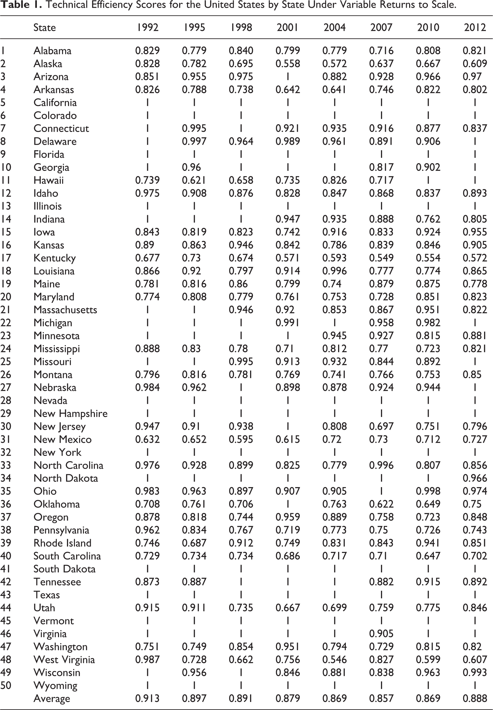
Comparing the efficiency scores over the twenty-one–year period shows that average TE for the United States has decreased. This decrease was consistent from 1992 until 2008. Since then, TE started to increase; however, by 2012, it did not reach the level of 1992. A summary of these results also shows that over the same period, twenty-two states became less efficient, and their output increased by a smaller scale than increase in all inputs (Table 2). Twelve states became more efficient, and the state’s output increased more than the increase in inputs. Sixteen states did not change in that their output increased by the same scale as increase in inputs. Interestingly, eleven of the sixteen were frontier states (FR) during the entire study period, and the other five were frontier states in 1992 but experienced a loss in efficiency by a small margin subsequently and by 2012 became frontier states again.

Table 2.

Summary of Technical Efficiency (TE) Scores by States Under Variable Returns to Scale.

Increase in TE (12)	Decrease in TE (22)	No Change in TE (16)
Arizona	Alabama	California (FR)
Hawaii	Alaska	Colorado (FR)
Iowa	Arkansas	Delaware
Kansas	Connecticut	Florida (FR)
Maryland	Idaho	Georgia
Montana	Indiana	Illinois (FR)
Nebraska	Kentucky	Michigan
New Mexico	Louisiana	Missouri
Oklahoma	Maine	Nevada (FR)
Rhode Island	Massachusetts	New Hampshire (FR)
Tennessee	Minnesota	New York (FR)
Washington	Mississippi	South Dakota (FR)
	New Jersey	Texas (FR)
	North Carolina	Vermont (FR)
	North Dakota	Virginia
	Ohio	Wyoming (FR)
	Oregon
	Pennsylvania
	South Carolina
	Utah
	West Virginia
	Wisconsin

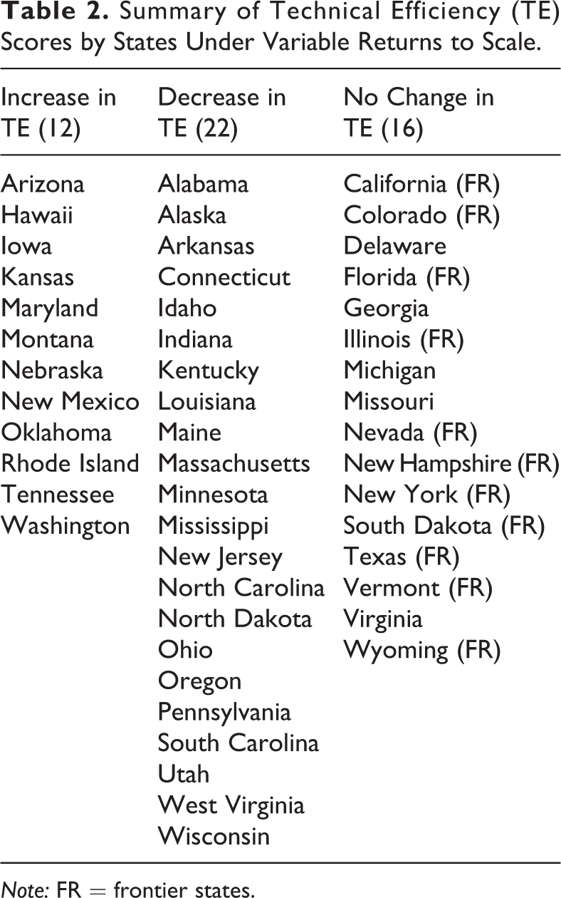
Note: FR = frontier states.

The results further demonstrate that states’ productivity, with some lag, followed the general trend in the economy. For instance, the aggregate economic condition was favorable for growth and expansion in the early to mid-nineties. Since then, the economy was growing at a sluggish pace until 2005, and the states followed this pattern. This was followed by a prolonged recession, which is reflected in the reduction in TE until 2009–2010. The official recession ended in 2009, and since 2010 a slow growth has been spurring and the economy has been showing signs of recovery, which are reflected in the increasing TE scores. The number of states with perfect efficiency scores of 1 decreased from twenty-two in 1992 to twenty in 2002 and eighteen in 2012. Less efficient states, where TE is between 0.75 and 1, increased in number from twenty-one in 1992 and in 2002 to twenty-six in 2012. The number of states with a TE less than 0.75, considered inefficient under DEA, went from six in 1992 to nine in 2002 and back to six in 2012.

Input Slacks

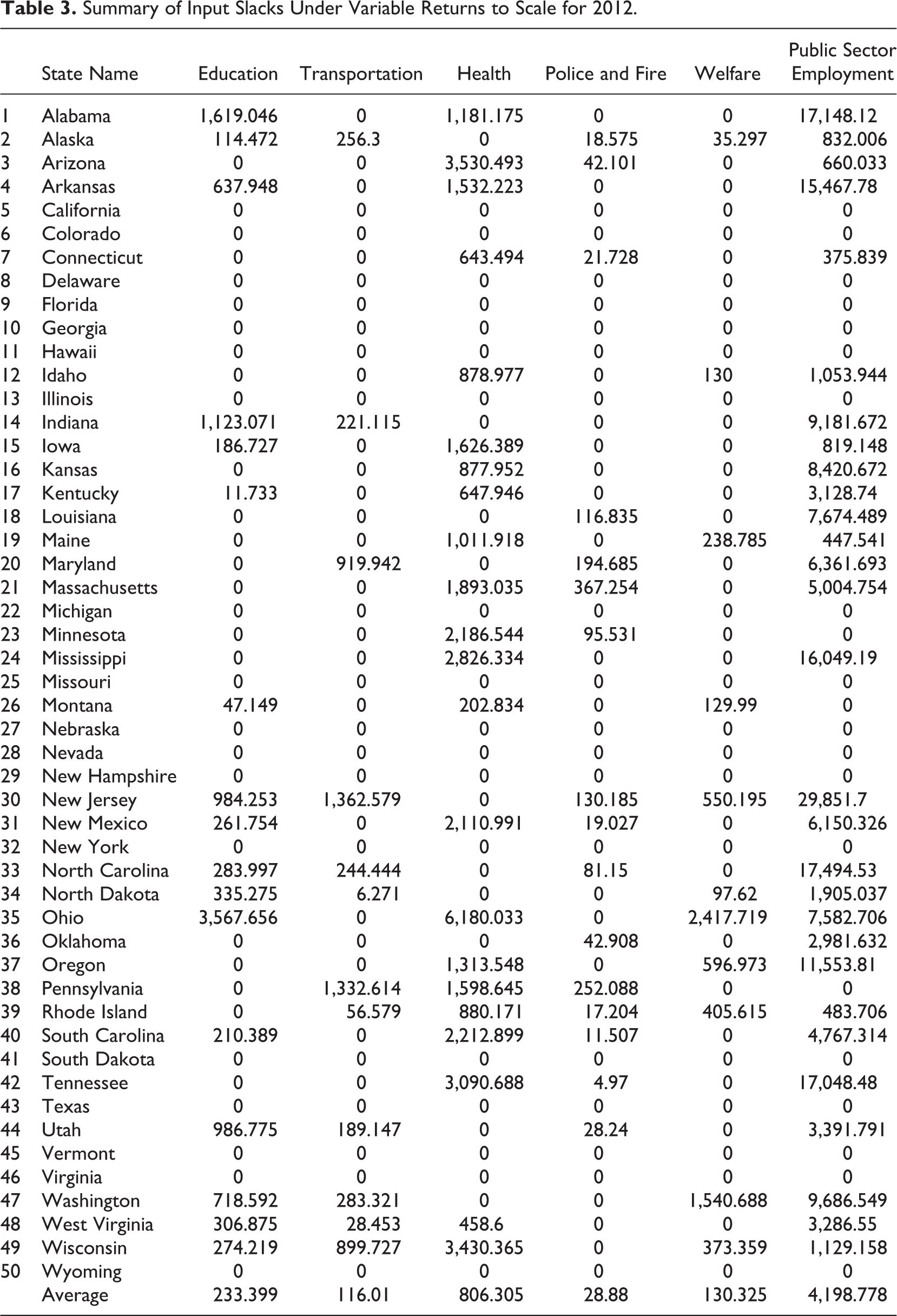
DEA allows for calculations of a measure that is useful in understanding the efficiency of the states: input and output slacks. Input slacks indicate the additional amount by which an input can be reduced or increased to attain TE after all inputs have been reduced in equal proportion to reach the efficiency frontier. Slacks with respect to output indicate the additional amount by which output can be increased to attain the efficiency frontier. Since the study focus was on input minimization, we were particularly interested in input slacks, that is, in determining how much input usage can be reduced to produce the same efficient output.

Table 3 shows the DEA input slacks under VRS for each state for each input for 2012. It provides a detailed picture for each state in terms of slack in the amount of expenditures in education, transportation, health, police and fire, welfare, as well as in the number of total employment. DEA estimates exact values by which each individual input can be reduced to produce the same amount of output for each state. For instance, in 2012, Alabama operated with TE of 0.821 under VRS (Table 3) meaning that the state could possibly reduce the consumption of all inputs by 17.9 percent without reducing output. In particular, the input slacks from Table 3 show that for Alabama to be efficient, it could reduce education expenditures by US$1,619 million, health expenditures by US$1,181 million, and total employment in government by 17,148 employees. In other words, if the state of Alabama could reduce inputs by the specified amounts, it would be as efficient as the frontier states. Similarly, for the same year, TE of Alaska was 0.609 under VRS, indicating that the state could possibly reduce consumption of inputs by as much as 39.1 percent. Thus, for Alaska to be efficient, it could reduce expenditures on education by US$114.5 million, transportation by US$256 million, public safety (police and fire) by US$18.5 million, welfare by US$35 million, and total employment by 832. In other words, if the state of Alaska could reduce inputs by the specified amounts, it would be as efficient as the frontier states, and so forth.

Table 3.

Summary of Input Slacks Under Variable Returns to Scale for 2012.

	State Name	Education	Transportation	Health	Police and Fire	Welfare	Public Sector Employment
1	Alabama	1,619.046	0	1,181.175	0	0	17,148.12
2	Alaska	114.472	256.3	0	18.575	35.297	832.006
3	Arizona	0	0	3,530.493	42.101	0	660.033
4	Arkansas	637.948	0	1,532.223	0	0	15,467.78
5	California	0	0	0	0	0	0
6	Colorado	0	0	0	0	0	0
7	Connecticut	0	0	643.494	21.728	0	375.839
8	Delaware	0	0	0	0	0	0
9	Florida	0	0	0	0	0	0
10	Georgia	0	0	0	0	0	0
11	Hawaii	0	0	0	0	0	0
12	Idaho	0	0	878.977	0	130	1,053.944
13	Illinois	0	0	0	0	0	0
14	Indiana	1,123.071	221.115	0	0	0	9,181.672
15	Iowa	186.727	0	1,626.389	0	0	819.148
16	Kansas	0	0	877.952	0	0	8,420.672
17	Kentucky	11.733	0	647.946	0	0	3,128.74
18	Louisiana	0	0	0	116.835	0	7,674.489
19	Maine	0	0	1,011.918	0	238.785	447.541
20	Maryland	0	919.942	0	194.685	0	6,361.693
21	Massachusetts	0	0	1,893.035	367.254	0	5,004.754
22	Michigan	0	0	0	0	0	0
23	Minnesota	0	0	2,186.544	95.531	0	0
24	Mississippi	0	0	2,826.334	0	0	16,049.19
25	Missouri	0	0	0	0	0	0
26	Montana	47.149	0	202.834	0	129.99	0
27	Nebraska	0	0	0	0	0	0
28	Nevada	0	0	0	0	0	0
29	New Hampshire	0	0	0	0	0	0
30	New Jersey	984.253	1,362.579	0	130.185	550.195	29,851.7
31	New Mexico	261.754	0	2,110.991	19.027	0	6,150.326
32	New York	0	0	0	0	0	0
33	North Carolina	283.997	244.444	0	81.15	0	17,494.53
34	North Dakota	335.275	6.271	0	0	97.62	1,905.037
35	Ohio	3,567.656	0	6,180.033	0	2,417.719	7,582.706
36	Oklahoma	0	0	0	42.908	0	2,981.632
37	Oregon	0	0	1,313.548	0	596.973	11,553.81
38	Pennsylvania	0	1,332.614	1,598.645	252.088	0	0
39	Rhode Island	0	56.579	880.171	17.204	405.615	483.706
40	South Carolina	210.389	0	2,212.899	11.507	0	4,767.314
41	South Dakota	0	0	0	0	0	0
42	Tennessee	0	0	3,090.688	4.97	0	17,048.48
43	Texas	0	0	0	0	0	0
44	Utah	986.775	189.147	0	28.24	0	3,391.791
45	Vermont	0	0	0	0	0	0
46	Virginia	0	0	0	0	0	0
47	Washington	718.592	283.321	0	0	1,540.688	9,686.549
48	West Virginia	306.875	28.453	458.6	0	0	3,286.55
49	Wisconsin	274.219	899.727	3,430.365	0	373.359	1,129.158
50	Wyoming	0	0	0	0	0	0
	Average	233.399	116.01	806.305	28.88	130.325	4,198.778

Conclusion

In conclusion, public sector efficiency has been a subject of discussion for a long time. This study has presented a fifty-state study of productive efficiency using DEA over a twenty-one–year period, from 1992 to 2012, involving several expenditures categories. The results of the study show that there has been a general decrease in efficiency during the study period, with some exceptions, based on both CRS (not shown) and VRS, which appears to be consistent with the growth trend in the national economy.

There are several advantages of using DEA to measure efficiency of state expenditures. For one, it would allow the decision makers to identify the states that are efficient as well as those that are not, when compared against the efficient (best practice) states. More importantly, the results produced by the method can help the decision makers improve allocation decisions by identifying areas where resources are over or underutilized to achieve efficiency. This is particularly important for governments that are financially strapped and find it difficult to carry out their expenditure activities, while trying to improve the well-being of their citizens. Similarly, public managers can benefit tremendously from the knowledge of the relative efficiency of public expenditures, especially when comparing different jurisdictions for similar services. This would allow them to identify what contributes to the variations in performance and what could be done to improve them. The public can also benefit from it: knowing how efficiently the government is able to provide services for their tax dollars would allow them to hold the government accountable when it fails to do so.

However, caution should be exercised in using the results as conclusive since the results provide a relative but not an absolute measure of efficiency. Another common concern with DEA is that, while the efficiency frontier lies at its core, it does not make a clear distinction between short- and long-term frontier. One could explain this, however, to persistent capacity utilization problem that can result from uncontrollable factors such as externalities over which the managers may not have sufficient control. Additionally, the constraints used in DEA include mostly observable inputs and outputs but not those that are unobservable such as jointness in production, which may require a broader interpretation of public goods. The method also does not address risks or uncertainties in service provision, although that may not be as serious a problem for the public sector as it is for the private sector. Interestingly, this is true not only of DEA but also of any quantitative study in government that uses empirical data.

Footnotes

Acknowledgments

The authors would like to thank the anonymous reviewers for their insightful comments and suggestions.

Declaration of Conflicting Interests

The author(s) declared no potential conflicts of interest with respect to the research, authorship, and/or publication of this article.

Funding

The author(s) received no financial support for the research, authorship, and/or publication of this article.

Note

References

Alchian

A. A.

1965. Some economics of property rights. Il Politico 30:816–29.

Aronson

J. R.

Hilley

J. L.

. 1986. Financing state and local governments. 4th ed. Washington, DC: Brookings Institution.

Aschauer

D. A.

1989. Is public sector productive? Journal of Monetary Economics 23:177–200.

Barnum

D. T.

McNeil

Hart

. 2007. Comparing the efficiency of public transportation subunits using data envelopment analysis. Journal of Public Transportation 10:1–16.

Barros

C. P.

2007. The city and police force: Analyzing relative efficiency in city police precincts with data envelopment analysis. International Journal of Police Science & Management 9:164–82.

Baumol

W. J.

1967. Macroeconomics of unbalanced growth: The anatomy of urban crisis. American Economic Review 57:415–26.

Bradford

D. F.

Malt

R. A.

Oats

W. E.

. 1969. The rising cost of local public services: Some evidence and reflections. National Tax Journal 22:184–202.

Buchanan

J. M.

Tullock

. 1962. The calculus of consent: The logical foundations of constitutional democracy. Ann Arbor: University of Michigan Press.

Charnes

Cooper

W. W.

Rhodes

. 1978. Measuring the efficiency of decision making units. European Journal of Operations Research 2:429–44.

10.

Coats

J. C.

2002. Applications of principal-agent models to government contracting and accountability decision making. International Journal of Public Administration 25:441–61.

11.

Coelli

T. J.

1998. Assessing the performance of Australian Universities using data envelopment analysis. Mimeo. Australia: Department of Econometrics, Center for Efficiency and Productivity Analysis, University of New England.

12.

Demsetz

1967. Toward a theory of property rights. American Economic Review 57:347–59.

13.

Downs

1957. An economic theory of democracy. New York: Harper and Row.

14.

Evans

Karras

. 1994. Are government activities productive? Evidence from a panel of US States. The Review of Economics and Statistics LXXVI:1–11.

15.

Farrell

M. J.

1957. The measurement of productive efficiency. Journal of the Royal Statistical Society, (A, general), 120:253–281.

16.

Forrester

2002. The principal-agent model and budget theory. In Budget theory in the public sector, eds. Khan

Hildreth

W. B.

, 123–38. Westport, CT: Quorum Books.

17.

Jensen

M. C.

Meckling

. 1976. Theory of the firm: Managerial behavior, agency costs, and ownership structure. Journal of Financial Economics 3:305–60.

18.

Johnes

2006. Data envelopment analysis and its application to the measurement of efficiency in higher education. Economics of Education Review 25:273–88.

19.

Gailmard

2010. Politics, principal-agent problems, and public service motivation. International Public Management Journal 13:35–45.

20.

Landau

1983. Government expenditure and economic growth: A cross-country study. Southern Economic Journal 49:783–92.

21.

Lane

J.-E.

2013. The principal-agent approach to politics: Policy implementation and public policy-making. Open Journal of Political Science 3:85–89.

22.

Leibenstein

1966. Allocative efficiency versus X-efficiency. American Economic Review 56:392–415.

23.

Mueller

D. C

. 1987. The growth of government: A public choice perspective. International Monetary Fund Staff Papers, 34 (March): 115–149.

24.

Munnell

A. H.

1990. Why has productivity growth declined? Productivity and public investment. New England Economic Review 1990:3–22.

25.

Niskanen

W. A.

Jr.

1971. Bureaucracy and representative government. Chicago: Aldin-Atherton.

26.

Nyhan

R. C.

Martin

L. L.

. 1999. Assessment of performance of municipal police services using data envelopment analysis. State & Local Government Review 31:18–30.

27.

Orzechowski

1977. Economic models of bureaucracy: Survey, extension, and evidence. In Budgets and bureaucrats: The sources of government growth, ed. Borcherding

T. E.

, 237. Chapel Hill: University of North Carolina Press.

28.

Pejovich

1969. Liberman’s reforms and property rights in the Soviet Union. Journal of Law and Economics 12:155–62.

29.

Plane

1992. Productive efficiency of public enterprises: A macroeconomic analysis based on cross-section estimation of a neoclassical production function. Journal of Applied Economics 24:833–44.

30.

Prakash

Rajesh

Thilagam

. 2012. Technical efficiency of state road undertakings in India—Data envelopment analysis. International Journal of Productivity Management and Assessment Technologies 1:31–42.

31.

Rassouli-Currier

2012. The relationship between institutional efficiency and instructional quality in higher education. Creative Education 3:224–27.

32.

Rutledge

R. W.

Parsons

Knaebel

. 1995. Assessing hospital efficiency over time: An empirical application of data envelopment analysis. Journal of Information Technology Management VI:13–23.

33.

Safdar

A. S.

2014. Measure efficiency by DEA model. Journal of Mathematics and Computer Science 20:253–57.

34.

Samuelson

P. A.

1954. A pure theory of public expenditure. Review of Economics and Statistics 36:387–89.

35.

Sav

G. T.

2012. Data envelopment analysis of productivity changes in higher education for-profit enterprises compared to non-profits. International Business Research 5:1–9.

36.

Spann

R. M.

1977. Public versus private provisions of government services. In Budgets and bureaucrats: The sources of government growth, ed. Borcherding

T. E.

, 71–89. Durham, NC: Duke University Press.

37.

Vining

Boardman

. 1992. Ownership versus competition: Efficiency in public enterprise. Public Choice 73:205–39.

38.

Warren

R. S.

1975. Bureaucratic performance and budgetary reward. Public Choice 24:51–57.

39.

Williamson

O. E.

1964. The economics of discretionary behavior: Managerial objectives in a theory of the firm. Englewood Cliffs, NJ: Prentice Hall.

Supplementary Material

Please find the following supplemental material available below.

For Open Access articles published under a Creative Commons License, all supplemental material carries the same license as the article it is associated with.

For non-Open Access articles published, all supplemental material carries a non-exclusive license, and permission requests for re-use of supplemental material or any part of supplemental material shall be sent directly to the copyright owner as specified in the copyright notice associated with the article.

0.00 MB

0.06 MB