Air Pollution in the Making

Abstract

This article traces an emergent tension in an interdisciplinary public health project called Weather Health and Air Pollution (WHAP). The tension centered on two different kinds of data of air pollution: monitored and modeled data. Starting out with monitoring and modeling practices, the different ways in which they enacted air pollution are detailed. This multiplicity was problematic for the WHAP scientists, who were intent on working across disciplines, an initiative driven primarily by the epidemiologists who imbued the project with meaning and value as the protagonists of “health.” To work collaboratively implies a stable, singular, and shared research object, however: one kind of data, one version of air pollution. In detailing two attempts by researchers to address the inadequacies of modeled and monitored data, this article explores the ways in which difference and multiplicity were negotiated and transformed. In doing so, this article suggests that it is the mobility and instability of data that are particularly fruitful for exploring the facilitation and enactment of new realities, while also making explicit the emergent problematics and partialities which inevitably result.

Keywords

data practices air pollution interdisciplinary research multiplicity difference

Introduction

As “epis” [epidemiologists] what we trust is when we see measurements, because we see it and we know how it works and that is a version of reality, but you might say it doesn’t represent all these different things. The epidemiologists don’t trust models, and the modelers, you say, you don’t trust the single point measurements. (Tim, Liaison meeting, May 18, 2012)

In this article, I analyze “the modeled and monitored data problem,” which divides researchers on the Weather Health and Air Pollution (WHAP)¹ project. Some are committed to using modeled data to study air pollution and its effects on human health, while others are committed to using data gathered by monitors. As an ethnographer on the project who was examining the practices and processes of knowledge production, I found the emergence of this question intriguing because, as the opening quote demonstrates, such terms as “true,” “good,” and “real” were used to describe data. These values struck me as pertinent because of their implication on the multiple kinds of veracity tied up with scientific inquiry. Within this interdisciplinary team, different groups of researchers held different views of what counted as true, good, and real data, and these variant perspectives were anchored in particular ways of coming to know air pollution and situated materializations of the research object (Mol 2002; Law and Mol 2002). For this project, the challenge of constructing interdisciplinary knowledge about the health effects of multiple air pollutions quickly became a practical and onto-political endeavor (Mol 2014; Stengers 2000), where the work of generating a shared air pollution involved modifying and materially intervening with its shifting relations and boundaries.

WHAP was an interdisciplinary public health project based across five different universities in the UK. With a methodological focus, the central aim was to draw together different kinds of data in ways that would enable relationships, patterns, and associations to be made about air pollution and health. The problem of different air pollution data did not only affect knowledge production but also forged relations to create and sustain a scientific entity called air pollution. That said, sharing and reusing different data were important ongoing issues for the researchers. As the introductory anecdote demonstrates, interdisciplinary discussions focused on different kinds of techno-scientific practices and the data they make possible. Further, the multiplicity of air pollution was a starting point for researchers themselves, not something revealed to them by the ethnographer through studying practice (Law and Mol 2002).

But such differences were managed carefully because of a shared interest in showing the health effects of air pollution. Health became both a moral imperative of doing relevant and useful research and a strategic way to demonstrate policy relevance and make tangible “impact.” The initially abstract notion of health influenced researchers to work as part of an interdisciplinary team and engage with diverse ways of understanding air pollution. A senior atmospheric chemist explained that

[…] you need disciplines to tell you what type of stuff is in particles, then if you want an estimate,…how much exposure does someone have living in Ipswich, what are they exposed to? […] we know how many people die in Ipswich, but there might not be a monitor there so you are going to have modelers to tell you, to derive a model for air pollution. So we might not have a monitor there but we know, because of the way the wind blows and where the emissions are coming from, we can tell you how much air pollution will be there. So you need a chemist, a modeler, you need as epidemiologist to be able to link the exposure and the health…so the question needs all those things. (Peter, interviewed on November 8, 2011)

Monitoring and modeling are two different ways of defining air pollution and producing and analyzing relevant data. Monitored and modeled data also exist side by side, used as comparative reference points for one another. In WHAP, their coexistence was challenging, primarily because the epidemiologists intended to reuse both data in ways that confronted monitored and modeled data’s particular boundaries, properties, and meanings. For example, the atmospheric chemistry modelers explained that modeled data are part of ongoing spatiotemporal fluctuations and therefore extracting a single measurement ignores the meteorological conditions and other chemical reaction of which it is a part. Monitors produce measurements of air pollution at particular points in time and space, particularly in areas considered to have high air pollution levels, and such data are seen as not measuring accurately the air that people actually breathe and are exposed to (background or “ambient air” is seen as the most representative measure of exposure).

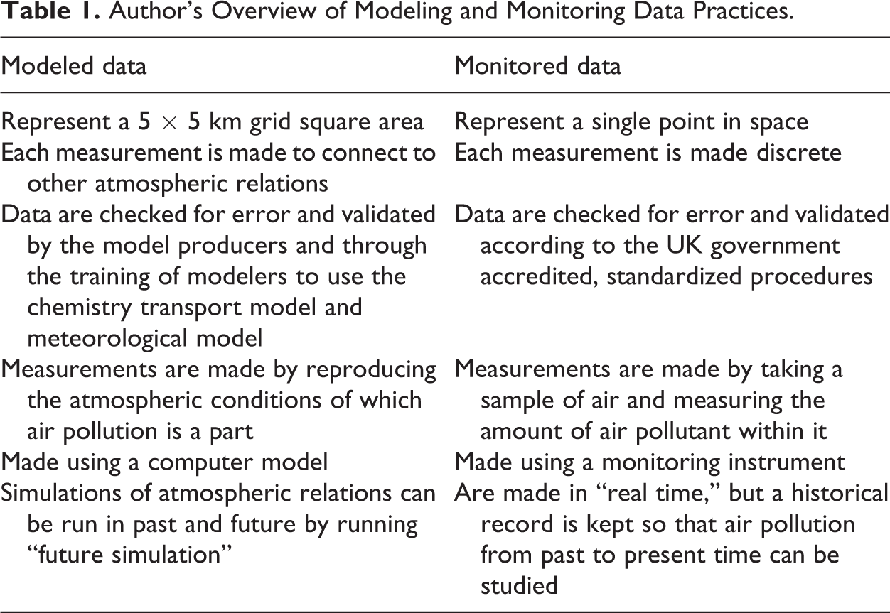
The atmospheric chemistry modelers on WHAP generated modeled data as part of their role in the project. The monitored data are publicly available data sets, however, and accessed externally by researchers through colleagues at a nearby university. The atmospheric chemists were keen for the epidemiologists to use their modeled data to study the relationship between air pollution and health. Modeled data were presented by the atmospheric chemists as superior to monitored data because they capture the complex interaction of atmospheric and meteorological conditions, rather than only generating data of air pollution at particular points in time and space (Table 1).

Table 1.

Author’s Overview of Modeling and Monitoring Data Practices.

Modeled data	Monitored data
Represent a 5 × 5 km grid square area	Represent a single point in space
Each measurement is made to connect to other atmospheric relations	Each measurement is made discrete
Data are checked for error and validated by the model producers and through the training of modelers to use the chemistry transport model and meteorological model	Data are checked for error and validated according to the UK government accredited, standardized procedures
Measurements are made by reproducing the atmospheric conditions of which air pollution is a part	Measurements are made by taking a sample of air and measuring the amount of air pollutant within it
Made using a computer model	Made using a monitoring instrument
Simulations of atmospheric relations can be run in past and future by running “future simulation”	Are made in “real time,” but a historical record is kept so that air pollution from past to present time can be studied

The conditions of interdisciplinarity of the project shaped the playing out of the research process and the particular ways data made a difference, influenced by epistemic cultures (Knorr-Cetina 1999) and modes of knowing. For the epidemiologists, the modeled data lacked the empirical veracity required to make valid, publishable statistical claims, proposing monitored data as a more viable and safe alternative. The personal careers of the researchers and their disciplinary backgrounds were also parameters of validation for data and research practices. For the modelers, the granularity of data necessitated by the epidemiologists in order to publish their results put into question the function and capacity of their European and global scale atmospheric chemistry models. The modelers’ more relational approach to studying air pollution shaped, and was shaped by, the kind of air pollution being imagined, where wider atmospheric processes were very much a part of materializing air pollution in time and volumetric space. In contrast, the epidemiologists wanted to ensure they were only measuring a single air pollutant in a controlled time and space. Their data carried meaning through a detailing of statistical methods that carefully sought to omit other environmental relations and interfering variables. The modeled and monitored data problem was therefore also constituted through these wider instrumental forces, which were played out through the negotiation of concepts like truth, good data, and what counts as a measure of air pollution.

“Looking Under Data”: From Representing to Intervening

As Bowker famously described, raw data is an oxymoron (2005, 184): you can’t separate data from the social––or what he calls the “raw” from the “cooked”––because data come from somewhere and are always situated (Haraway 1988). Data are particularly useful objects for tracing the making of epistemic and ontological boundaries. “Looking into data, or better, looking under data to consider the root assumptions” (Gitelman and Jackson 2013, 5) contributes to our descriptions of the ongoing changes to the material, social, and ethical conditions of scientific inquiry. I found that data enabled exploration of the movement, translation, and openings between practices of knowing and doing, and thereby the making of spaces for materializing air pollution as an interdisciplinary concern. Using data to manage multiple ways of knowing air pollution meant data were also “digital devices” (Ruppert, Law, and Savage 2013), which were productive and performative of interdisciplinary research.

In Science and Technology Studies (STS) and anthropology, it is now a well-rehearsed argument that no object or phenomenon is singular and that material practices enact different versions of objects in practice, bringing them into being in multiple ways (De Laet and Mol 2000; De la Cadena et al. 2015; Gad, Bruun Jensen, and Ross Winthereik 2015; Harvey et al. 2014; Jensen 2004; Latour 1999; Law and Mol 2002; Mol 2002). Accordingly, how to describe and manage the relations between different knowledge practices requires paying attention to the local collaborative dynamics established between different methods and forms of labor (Moreira 2006). Some of the tensions that emerge when practitioners from different fields of practice work together have been well examined (Star and Griesemer 1989; Edwards et al. 2011); Mol (2002) has focused on the ways in which multiple ontologies somehow “hang together.”

Attending to the “partial relations” (Strathern 1991) between data and their continual multiplying was a point of departure both for myself and the scientists on WHAP. Much STS research assumes that discussions about reality stem from our own detailing of ontological clashes. Implicit in such accounts is the assumption that these clashes are invisible to the practitioners themselves (Law and Mol 2002). Yet, as Stengers (2005, 184) writes, studying practice means approaching practices as they diverge, “that is, feeling its borders, experimenting with the questions which practitioners may accept as relevant.” In WHAP, workings of reality were explicitly acknowledged and engaged with by the team. What counted as good data came under scrutiny, so that data practices didn’t simply involve collection and use, but also included deliberations over what data mean in particular circumstances, and how different data could be used effectively across practices. In doing so, data became a way to refigure the conceptualization and practical management of difference (specifically, different air pollutions) as an interdisciplinary (and ethnographic) problem.

Rather than considering data as the end point of research, I understood it as processual and enactive of knowledge making. Accordingly, in the account that follows, data function as both representations that embody ways of knowing while also operating prescriptively as particular kinds of engagements with the world. This shift from knowing at a distance to materially intervening is one that resonates with Hacking’s (1983) coupling of representing as intervening, blurring the lines between coming to know objects, and actively configuring them. In WHAP, the ways in which researchers sought to classify work as relevant or problematic, real, or applied shaped the kinds of realities about air pollution that emerged, and thereby what was made invisible/visible and significant to the problem of air pollution. Seeing data as device was therefore an aspect of method particularly pertinent for exploring realities in the making and the ontology of the digital (Knox and Walford 2016) more generally. Studying science through data and other such processes means that articulations of truth and reality become evolving and contingent. Inquiry into these processes offers an opportunity to trace the affordances, agencies, and logics of different data as they participate in the making of social worlds (Knox and Walford 2016).

Researchers on WHAP were not only interested in air pollution (what it is, how to measure it, and what the resulting data mean) but also crucially interested in the relationship between air pollution and human health (in what ways air pollution relates to other phenomena). It was due to the targeting of health in their aims and objectives that the project’s funding bid was successful, and health was the means by which they would ultimately demonstrate “impact.” As one senior modeler explained, “it is all very well making these beautiful plots but we want to know what it all means, how does it affect health?” It was the role of the epidemiologists to describe this link. Their specific focus was on the short-term effects of air pollution. Through the statistical exploration of air pollution data (modeled or monitored) with health data from the Office for National Statistics (mortality) and the Myocardial Ischaemia National Audit Project (MINAP²; morbidity, specifically, heart and lung disease), correlations between “health events,” such as increased hospital admission for a heart attack or decreased lung function, with “air pollution events,” like high levels of ozone, could be made. The relationship between high air pollution episodes and changes in population health was used to understand patterns of environmental health and measures of risk for public health policy and intervention.

In order to study air pollution and health relations, it is necessary first to decide what data of air pollution to use. The first option proposed was monitored data, which instigated a series of attempts to find new, better kinds of data of air pollution. The modelers on WHAP generated modeled data, and this led to a series of comparisons of monitored and modeled data. The epidemiologists were keen to ensure the air pollution data were, first, enacting the right kind of air that people breathe (spatially) and, second, that these data were “empirical” and not “too mediated” by technologies and people. As already detailed, what counted as good air pollution data was different for the modelers, and these gaps and fissures were often described as types of “error” by researchers. Yet how good data were defined and error managed generated new encounters, queries, and material concerns and, as I will discuss below, through these processes air pollution emerged as an interdisciplinary phenomenon.

Monitored Data (the Extraction of Air Pollutants)

The epidemiologists began by explaining to the team the problem of using monitored data [referred to as measurements] in their analysis of the health effects of air pollution. One reason, they suggest, is that “we only have measurements in a limited number of grid squares.”³ This is problematic because they are measuring the health effects across the whole of the UK. The second problem is that the modeled and monitored data “aren’t measuring quite the same thing,” “we are not going to have the gold standard” and “we are not comparing like for like and it is a struggle to try and address this”. (Field notes, Liaison meeting, April 2, 2012)

Air pollution is monitored across the UK, initiated by central government and often carried out by local councils. Discrete measurements are collected at different sites, organized into geographical networks. For example, London has one accredited air quality network managed by government departments, local councils, university research groups, and environmental agencies. The aim of these automated technical systems is the production and maintenance of “continuous data.” This means that past-to-present data on air pollution are collected, sustained through the data network (from production to storage) in order to make up what was referred to as a “data archive.” The purpose of these data is to provide the public and authorities “real-time” information on current air pollution levels and to enable short- and long-term responses to air pollution as a public health concern (Department for Environment, Food and Rural Affairs 2012).

Monitoring stations are small cabins containing a number of different air pollutant monitors (Figure 1). These monitors draw samples of surrounding air in through tubes that connect the inside of the station to the ambient air outside. Once in the tubes, the air samples go through a process of purification, where the parts of air not being measured are taken away with a scrubbing device. This construction of the object of interest as discrete in space and time meant the sensor was able to measure the pollutant inside the monitor. The sensor functions with the passing of an ultraviolet light beam through the tube, and the measure of the pollutant is the measure of the reaction that results from this process. The final data are expressed as parts per million, which can be converted to micrograms per cubic meter (µg/m³). For particulate matter (PM), sizes are expressed in micrometer in diameter, generally as PM₁₀ or PM_2.5.

Figure 1.

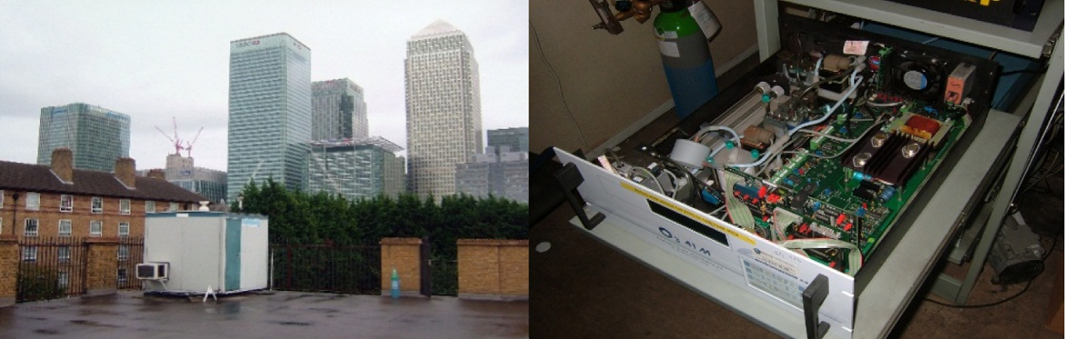
Inside a monitoring station (personal photo).

In order for these numbers to be turned into data, the numerical readings are checked to ensure they are measuring the “right relations” of air and have not been unduly influenced by the instrument used. Routine calibration tests are one key way to ensure the validity of data. In a calibration test, the air sample is measured and compared with a laboratory certified standard, stored in gas canisters within the monitoring station. Ideally, the readings on the front of the monitor should be the same as the measure in the gas canisters. Looking for this “span and drift” of the measurement made in comparison to the certified standard is a way to check the effectiveness of the instrument, as site technician Phil explained: “I am looking for the readings to stabilize […] so to stay at around the same number to check all is functioning ok” (Field notes, October 25, 2012). These descriptions are recorded and input into the spreadsheet and contribute to what Phil explicitly referred to as “a record keeping exercise” that ensures the continual archiving of monitoring air from past to present. The calibration results are attached to the measurements made by the monitor, so that they can be drawn upon to check and explain the measurements (and, accordingly, make any adjustments required) at a later date and in subsequent data analyses carried out off-site.

Some of the defining features of monitored data were problematic for the epidemiologists on WHAP, however. First, monitors were often described as only measuring air pollution levels from particular sources, like traffic, often located in places considered to have poor air quality rather than “the kind of air people breathe.” One concern related to checking data was that the monitors picked up higher levels of pollution than people are likely to breathe (if monitors are located on roadsides, for example). The epidemiologists grappled with this by comparing monitors on roadsides with monitors located in spaces described as “background air” in order to work out whether the margin of difference between these measurements could be significant to measures of health risk. Second, monitors only measure air at particular spatial points and therefore do not capture all the different types of air people breathe in space and time. Indeed, it is widely recognized that individuals’ exposure changes as they move, for example, from inside their home to the bus stop and to and from work (Gulliver and Briggs 2005; Laumbach, Meng, and Kipen 2015; Myers and Maynard 2005). Epidemiologists regarded these discrepancies as reducing their ability to measure variation in exposure of human populations across the UK. Their aim was to make visible the temporal sequence, and thereby potential correlation, of air pollution and health in predefined mapped spaces through time-series analysis. If the measurement generated by a monitoring station differs from the exposure of an individual a few 100 m away, then the subsequent statistical linking of air pollution data with health data may generate inaccurate correlations.

Modeled Data (Maintaining the Relations of Air)

Time-series studies use daily means in background monitors as proxies for residents living nearby […] The epidemiological gold standard might be the concentration over parts of the grid (5 × 5 km grid square) in which people breathe. Current assumptions are that monitors are randomly placed over those areas––or at least randomly sample the pattern of the series of daily observations (means matter less to us). The [modeling group] have queried this assumption, suggesting that the background monitors are typically more affected by traffic than typical residential areas. Apart from it being an issue for us in assessing suitability of model (and monitor) series for epidemiology, it is arguably an issue of general importance in interpreting monitor concentrations. (Peter, internal e-mail, March 15, 2013)

Modeling was proposed by the atmospheric chemists as a practice that addresses the inadequacies of monitoring by generating data that take into account the spatiality of air pollution. The model is three dimensional and therefore measures volumetric space rather than air pollution on the ground or at a surface level (like monitoring stations). Each three-dimensional volume box calculates emissions, the pollutant concentration in the atmosphere postemission, its interaction, chemical transportation, and any secondary products as result of ongoing atmospheric and chemical reactions. This attention to process and movement takes into account the changing concentrations of pollutants as part of atmospheric relations. The modelers explain that “the model calculates these [changes in concentrations of air pollutants] at every step […] the monitored data may be the truth and accurate, but it doesn’t reflect the 5 × 5 km grid” (Tom, modeler, December 13, 2011).

The simulation model used in WHAP was a combined chemistry transport model (CM) and weather model (WM). This CM-WM was used by the atmospheric chemists to simulate the concentration and movement of air pollutants in the atmosphere, generating three hourly descriptions (by mathematical equation) of the evolution of the dependent variables (the parameters and boundary values) of the model (project protocol). The movement and flux of pollutants are influenced by meteorology and atmospheric processes, and the model is a theoretical representation of these assumptions described through mathematical equations.

By typing out instructions in the command box visualized on a computer screen, Craig, the main modeler in WHAP, manipulated the modeled atmosphere to produce a measurement of a particular air pollutant. Communicating with the model through computer code, he arranged the designated variables of interest in ways that generated concentrations of air pollution––µg/m³ air (one-millionth of a gram)––according to the desired frequency (usually hourly or daily). This process was also iterative and involved managing and responding to error in these output files. Addressing errors was a major component of ensuring that the maps visualized the right kind of atmospheric relations. It was both the numerical output and the visual forms (Figure 2) that were used to determine what counted as good data.

Figure 2.

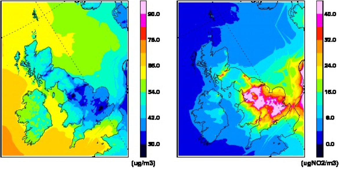
Mapped color visualizations of changing air pollutant concentrations.

Instead of tubes and sensors, for modeling the measurement context was built with computer code, so the complexities that make up controlled environments, such as temperature, weather conditions, and time, were incorporated into the model (Garnett 2016). Here, modeling seems like an additive process through which relations were made in the building and running of a computer simulation of the atmosphere (where error emerges). Concentrations of air pollution were considered as composed and comprised within these physical and chemical interactions. The relational nature of atmospheric processes shaped the descriptions used to characterize the modeled data, such as “volume mixing ratio” or “pollutant depositions.” This contrasts with monitoring, where the air pollutant was made pure by “scrubbing” other parts of air away.

Nonetheless, for the epidemiologists, the modeled data were “simulated” and therefore “not empirical.” They insisted that modeled data were also problematic for their study of air pollution and health despite the modelers’ claims that their data more accurately captured the 5 × 5 km grid square. Monitors were described as “outside” and “on the ground,” which was considered as implicative of their effective capturing of the air to which people are exposed. This made the monitoring data alluring. As Principal Investigator, Tim explained, “what we trust is when we see measurements, because we see it and we know how it works and that is a version of reality” (Tim, Liaison meeting, May 18, 2012). The epidemiologists also had close colleagues at a nearby university who conducted the cleaning procedures and validity was assured through this wider network of local expertise. Second, as has been highlighted, the conditions of air at monitoring sites were thought to correspond to the air that people breathe and therefore more relevant for research on health. This latter point is differentiated by the chemical conditions of air and particular ideas of human exposure and health. The epidemiologists considered the air that people breathe different to wider atmospheric processes and chemical reactions. Again, this highlights the different kinds of air, and therefore material framings of the problem of air pollution, that are mobilized through an engagement with different data as a result of interdisciplinary research practices.

Solution 1: Adding Modeled and Monitored Data Together (Data Assimilation)

As a result of these detailed “shortcomings” of modeled and monitored data, the epidemiologists proposed adding modeled and monitored data together as a way to counter the inadequacies of each:

[W]ith two independent approximate estimates (model- and monitor- based) it should be possible to get a better estimate by assimilating the information from the monitors with that from the model […] and that the epidemiological world seems skeptical of using modelled data on its own (at least for time-series analyses) adds motivation to consider this. (Team-wide e-mail, November 13, 2011)

This was a rather tentative suggestion. Peter, the main protagonist of the data tension, referred to “other studies” which could be used to think about doing data assimilation, resulting in a rather vague summing up: “the basic idea of data assimilation is that two sorts of data are combined in order to produce more valid data.” By adding data together and working out the average of these two kinds of measurements of air pollution, a more accurate representation was made possible. Moreover, the epidemiologists hoped they could then use “real-time” monitored observations alongside the modeled data made by the atmospheric chemists on WHAP, thereby addressing potential concerns within the wider epidemiological community as well as fulfilling requirements of their co-collaborators.

In practice, data assimilation is the process by which observations of the “actual system” are incorporated into the numerical model of that system. The epidemiologists explained that by adding both modeled and monitored data of particular pollutants an average of the two could be used to counter the discrepancies in each. However, the modelers responded by stating that they could not simply add monitored data to modeled data without remaking the atmospheric relations tied up with the pollutant measured. This would involve, for example, changing the emissions data used to build the model in order to make the input data relate to the assimilated output measure correctly. Both these actions would require the involvement of other researchers, data sets and a transformation of the model itself, rather than simply its reuse.

One modeler, Tom, made two important points relating to the epidemiologists’ suggestion of data assimilation, highlighting the ways in which it challenged the boundaries, properties, and meanings of modeled data, specifically in terms of simulating future air pollution scenarios:

[The] epis are not so much interested in the science of it all but more so in making sure the grid square matches the measurements. This means that even if the model is a load of rubbish or not working properly, it doesn’t matter. However, this causes problems in the future because if you want to use future scenarios, like we are in WHAP, then if the model has got problems then it won’t work. (September 9, 2012)

Accordingly, assimilating, and therefore attempting to match modeled and monitored data, was not a sure way to check validity, because correspondence does not acknowledge differences within the model. Second, the data produced by the model pertain to the model itself and cannot simply be detached from this relationship by integrating it with monitored data. In this sense, the same is always different, and finding similarities between data (the aim behind assimilation) generated new kinds of difference––in terms of different types of validation procedures and different kinds of workable realities for data making. In monitoring, air pollution is a matter that responds to measuring urban environments where citizens move and breathe. For the modelers, air pollution is part of a complex and global intra-acting system rather than a discrete phenomenon.

The epidemiologists’ assumption that assimilating data would increase validity was disputed by the modelers, who claimed that “correspondence” (similarities and differences between kinds of data) may belie “noncoherence” (differences within data). Modeled data are situated and relate to the model to which it is attached. It cannot simply be detached from this relationship and integrated with monitored data because new discrepancies arise. “Simulated reality” is different to the epidemiologists’ “empirical reality” because internal coherence was valued at the cost of external correspondence. For the epidemiologists, pollutants were considered as distinct and interrelated rather than relational (and co-constitutive) because of this need to construct “exposure–response” relationships⁴––that is, exposure (to one kind of pollutant) and response (individual health effects) relationships. Bringing modeled and monitored data together into a shared research space made explicit the ontological tension around what and where air pollution is, challenging the implicit emphasis of interdisciplinary research and overarching aim of producing knowledge on a shared object of concern.

Solution 2: Combining Modeled and Monitored Data (Particularizing Air Pollution)

Using pencil and paper [the statistician] begins by sketching out and explaining how she sorts out databases of modeled and monitored data on an Excel spreadsheet. I am told there are only about ninety monitoring station sites, which means they [the epis] can make comparisons with modeled data [modeled data are produced for every 5 × 5 km grid square] in relatively few areas. In Excel, the comparison is carried out to produce 3-4 time-series of modeled and monitored data. From this comparison, measures of error are made and these can be statistically removed in order to produce a true data set. I question how this is a “true” data set and the statistician explains that it is true because the error has been removed. The true data set can then be compared with modeled and monitored data, and the results of this comparison are a way to confirm which data is best [with the least error] for their study. (Field notes, September 12, 2012)

Since the idea of data assimilation was rejected by the modelers, Tim, the PI and a senior epidemiologist, suggested a “conceptual approach” to work out which data are best in relation to their own respective epidemiological data practices. This conceptual shift oriented discussions toward a new kind of data practice called “the simulation study.” In the simulation study, the statistical framework of time-series regression was used as a means for comparing two sets of modeled and monitored data (2000-2010). The statistician working on the time series explained that she used monitored data from a data set the epidemiologists had used in a previous study and a work in progress modeled data set from the atmospheric chemists on WHAP.

As the opening anecdote details, arranging the two kinds of data in Excel enabled their comparison within the new data practice of time series regression. The modeled and monitored data become situated there, and the data compared in terms of how they function as part of this new data practice. A comparison of ozone and NO₂ was carried out first because the relationship between these two pollutants is well known (Clappa and Jenkin 2001). By detailing how these air pollutants will behave, the model and monitor were judged in terms of how closely they captured such established chemical relationships. The simulation study used the known relationship in an attempt to understand how well models and monitors measure air pollution.

Paramount for the epidemiologists were the ways that error influenced the measurement of air pollution and therefore the representational veracity of data. The statistical equations only work if a “truth” can be used, where E_b and E_c stand for error types––“Berkson” or “Classical” (see Figure 3). As the statistician explained, they make “true data” of air pollution by taking into account these classified measures of error and subtracting error from each data set via Excel (“the calculating tool”). This true data could then be used to see how error influences the measurements of air pollution made by models and monitors. Generating measures of error and thereby constructing true data was a situated practice of making epidemiological data of air pollution.

Figure 3.

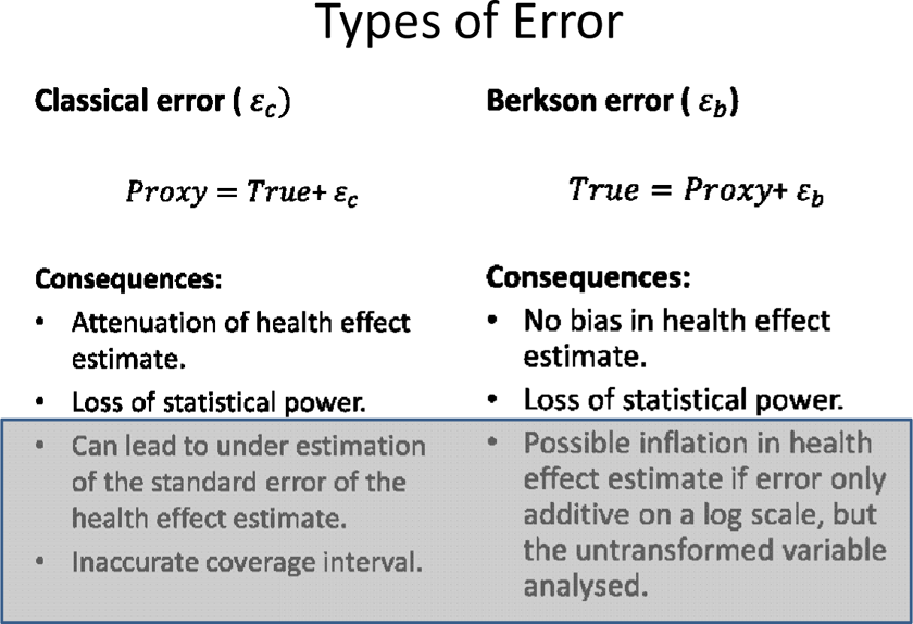
The classification of error. Source: Weather Health and Air Pollution team meeting slides, June 6, 2013.

The defining of error also generated a new way of understanding and arranging data that could be used to contribute to the modeled versus monitored data issue. The modeled data error (Berkson error) was described as “not precise” because the error was not only about the spatial siting of the instrument, like monitors, but also about the error within the model itself and the “misclassification” of air pollution. The measures of error became a way to classify different versions of air pollution in data. This was described as an “unknown unknown,” a term used by the epidemiologists to describe error that they cannot measure. Classical error, however, refers to discrepancies in the spatial representation of air pollution (it is a gap in the remit of data’s spatial capture) rather than the theoretical representation of air pollution (the differences within air pollution as a research object), which can be measured and taken away by the epidemiological model through the introduction of relatively simple equations (coined as a “known unknown”).

The simulation study not only classified data according to standardized ways of conceptualizing error in epidemiology but also materialized a way of judging data practices according to their locally made simulated true data. These new data intervened in the tension by becoming a reference point from which a standard of “good data” for comparing modeled and monitored data could be achieved. Moreover, the data became a way to prove which data were best (within WHAP), and functioned as justification for the data used in the final epidemiological analysis (for the wider academic community).

Measuring Difference

The epidemiologists were interested in the relations between air pollution and health, and these were conceptualized as two distinct empirical phenomena. Health was a proxy for measures of mortality and morbidity. This was framed in different ways, from “quality-adjusted life years” (QALY) to “years of life lost.” As a quantified qualitative value, health was something that related to an individual human body and its state as alive or dead. In terms of morbidity, health became a measure of disease burden, and QALY, for example, also the measure of socioeconomic costs of ill-health. In order to map air pollution and health over time, daily measures of air pollution for particular spatial areas (postcoded 5 × 5 km grid squares) were linked with hospital and mortality data. Increases or decreases in mortality and morbidity on particular days could then be examined with data of air pollution levels.

The simulation results didn’t demonstrate that either data were better in any concrete or decisive way, however, as Peter explained:

On presenting some of the technicalities of the simulation study to the team, Peter describes their implication for the epidemiology group, claiming that: “for ozone, monitors are always better than models and for NO₂ neither monitor or model perform well”. (Team meeting, December 6, 2012)

As mentioned above, it is well known that ozone is directly related to nitrogen oxides (NO_x). ozone (O₃) forms through the generation of oxygen atoms from the splitting of nitrogen dioxide (NO₂) by sunlight. Most atmospheric NO₂ is emitted as NO, which is rapidly oxidized by ozone to form NO₂. As secondary gases, O₃ and NO₂ are tricky to measure because their reactions are shaped by the composition of the atmosphere and meteorology. This means that their concentrations can fluctuate rapidly over the course of a day. Despite fluctuation over time, O₃ remains stable in geographical space, which means monitors function well because the measurement taken is likely to be representative of, in our case here, a 5 × 5 km grid square. It was the spatial stability of ozone that led the epidemiologists to confirm that monitoring data produces better data than the models because monitors are physically stable in space and time. Yet the toxicity of NO₂ is located in its interactions with other pollutants, which means that concentrations and point measurements are less accurate for measuring exposure and health effects. Indeed, time-series models are not recommended for this pollutant because of its high correlation with copollutants (World Health Organization 2005). NO₂ was not well measured by the monitoring station or the model, according to the simulation study; yet monitored data still trumped modeled data at this stage.

It was the complex and heterogeneous pollutant PM that led the epidemiologists to confirm that they would, after all, also use modeled data. The finer particles, PM_2.5, with a diameter of less than 0.25 µm, were indistinguishable by monitors that measure PM by weighing the mass of particles rather than detailing the heterogeneity of particles like the model (Figure 4). It was the capture of the multiple kinds of particulates and unpacking their chemical characteristics that made modeled data so appealing, especially in light of a growing awareness of the negative health effects of PM (Milojevic et al. 2014, 1096).⁵ Rather than mixing modeled and monitored data within data practices, the simulation study results led the epidemiologists to use modeled data for some pollutants and monitored data for others because relatively few monitoring stations measure the pollutants of interest, PM_2.5: “in many cases modeled data is the only game in town” (Peter, team meeting, June 13, 2013).

Figure 4.

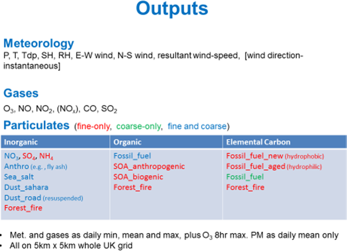
Chemistry transport–meteorological modeling outputs. Source: Atmospheric chemist’s presentation, team meeting, December 6, 2012.

The simulation study generated data on the veracity of modeled and monitored data by measuring the particular kinds of error generated in these data practices. The simulation study did offer a solution in the sense that each kind of data was used by the epidemiologists but in different analyses of particular pollutants: monitored data for ozone and NO₂, modeled data for PM_2.5. The potentiality imbued in the practice of the epidemiological reuse of data was an opportunity to define the differences within data in ways that enabled the boundaries, properties, and meanings of data to shift. Modeled and monitored data were not used together––either through addition (data assimilation) or in their combination (within the simulation study data). Furthermore, modeled and monitored data remained separate in the epidemiological analyses, with particular time series generated for particular pollutants. This meant that particular versions of air pollution were made and sustained. The multiplicity of air pollution did not “hang together” (Mol 2002) here but rather became the starting point for further articulations of air pollution while also transforming the very definition of difference.

Diffracting Air Pollution with Data

[…] mapping of interference, not of replication, reflection or reproduction. A diffraction pattern does not map where differences appear, but rather maps where the effects of difference appear. (Haraway 2004, 70)

The conceptual condition of the mobility and instability of data is particularly useful for considering how differences emerge and particular ontologies get enacted. It was through the data practices of WHAP, their arrangements, and orderings, that the “cooking” (Bowker 2005) of data was made apparent. Cleaning data and making it error free were central components of data in process, and the anecdotes drawn upon in this paper present a detailing of the work that goes into making data usable. Indeed, it was not only differences between data but differences within data––from truth and error to their spatial representations, that shaped how data were used, shared, and articulated. Moreover, the internal differences within data opened up alternative ways of making data, which then enabled data’s reuse in ways that refigured air pollution.

One key distinction used by the epidemioloigsts to define data was that of “the empirical” (true) and “the modeled” (constructed)––a binary analogous to that of the raw and the cooked (Bowker 2005; Gitelman 2013). According to Levi-Strauss (1983; see also Boellstorff 2013), cooking implies social and cultural shaping, whereas raw designates the natural and unprocessed. Of course, our construction of natural fact and reality need to be constantly assessed (Latour 2004), as was the case in WHAP, where what counted as raw or cooked data came under scrutiny through the coalescing of different disciplinary practices. The epidemiologists considered the monitored data as less cooked than the modeled data and therefore “more real,” yet the cleaning, or cooking, of data was not openly discussed by the epidemiologists. This suggests that it was not the making of data that mattered to the epidemiologists but rather its essential form and meaning according to their ideal of empiricism. The atmospheric chemistry modelers, in contrast, argued that monitoring data are also cooked, but they are cooked differently to modeled data, which, they claimed, was more open and responsive to air pollution in flux and motion.

The theme of cooking became a topic of interest for the team. The making of modeled data was made explicit, and the accounting for related atmospheric relations meant air pollution was co-constituted through meteorological and chemical processes. In monitoring, cooking required losing such relations. Neither data were raw but the result of an active engagement and modification of data in the in-between stage of emergence and becoming. In addition, air pollution’s capacity to overflow attempts to contain and stabilize it meant that air pollution was also continuously producing an “other” with respect to measuring practices. Focusing on the transformations of data highlights how data of air pollution (re)make difference in ways that are generative of new kinds of questions about air pollution.

The shifting debate between researchers about whether versions of the real were “useful” (what cooking does) could not be resolved by team members but was instead managed through data practices. The epidemiologists ultimately claimed which data were best according to the particularities of pollutant types. Differences between data of air pollution were not reduced but remade in the playing out of the modeled and monitored data problem. This process facilitated new kinds of relations and attachments (e.g., linking ambient air with diseased bodies), while also giving rise to new problematics and partialities (e.g., how to spatially and temporally bound the air that people breathe for measurement). Data were not made to “hang together” (Mol 2002) but became further entangled. For example, the notion of data assimilation was problematic for the modelers, as were the measurements made by monitoring stations, but these data were reworked in ways that made them valid for epidemiological research, which meant that health claims about air pollution became possible. These different ontologies of air pollution were at once contested and made to coexist. Difference was harnessed, and rather than an absolute boundary they functioned more like an iterative and inventive process of further differentiation and entanglement, or what Haraway calls “diffraction” (1997).

Data were both the object of research and means by which researching was practiced, so that epistemic and ontological concerns became entwined, embedded, and inscribed in and through the practical work of making and reusing data. Difference and ongoing differentiation were not external to data enactments but rather internal to them (Knox and Walford 2016; see also Holbraad, Pedersen, and Viveiros de Castro 2014), which is illustrative of the ways in which data can be distorted and transformed to compose new possible realities. Difference was altered by focusing on the cooking of data because how particular data become different through practical work can be traced and understood. This attendance to the internal differences of air pollution through careful crafting builds on Mol’s argument about the politics of multiplicity by highlighting the methodological dimensions of making difference together: there were not only different versions of air pollution in WHAP but also transformations (or diffractions) of the arrangements that sustain them. The emergent nature of data in interdisciplinary research allowed WHAP researchers and me to elicit difference partially but also in inventive ways, thereby bringing new entities and relations into existence: establishing new aims and objectives (from air pollution to health) and enacting the meaning of data through different practices (from true data to useable data) in ways that shifted how air pollution could be known.

Footnotes

Author’s Note

Ethical approval was granted by the London School of Hygiene & Tropical Medicine Ethics Committee.

Acknowledgments

Special thanks to researchers on the WHAP project, whose patience and support made this research possible. Thanks also to Judy Green, Catherine Montgomery, and Simon Cohn for guidance during the course of the PhD, on which this work is based, and to the two anonymous reviewers for their comments that greatly improved this article.

Declaration of Conflicting Interests

The author(s) declared no potential conflicts of interest with respect to the research, authorship, and/or publication of this article.

Funding

The author(s) disclosed receipt of the following financial support for the research, authorship, and/or publication of this article: Fieldwork for this research was supported by the Natural Environmental Research Council, UK.

Notes

References

Boellstorff

Tom

. 2013. “Making Big Data, in Theory.” First Monday 18 (10).

Bowker

Geoffrey

. 2005. Memory Practices in the Sciences. Cambridge, MA: The MIT Press.

Clappa

Lynette J.

Jenkin

Michael E.

. 2001. “Analysis of the Relationship between Ambient Levels of O3, NO2 and NO as a Function of NOx in the UK.” Atmospheric Environment 35 (36): 6391–405.

De la Cadena

Marisol

Lien

Marianne E.

Blaser

Mario

Jensen

Casper Bruun

Lea

Tess

Morita

Atsuro

Swanson

Heather

Ween

Gro

West

Paige

Wiener

Margaret

. 2015. “Anthropology and STS: Generative Interfaces.” Hau: Journal of Ethnographic Theory 5 (1): 437–75.

De Laet

Marianne

Mol

Annemarie

. 2000. “The Zimbabwe Bush Pump: Mechanics of a Fluid Technology.” Social Studies of Science 30 (2): 225–63.

Department for Environment, Food and Rural Affairs. 2012. Automatic Urban and Rural Network. Accessed February 25, 2016. http://uk-air.defra.gov.uk/networks/network-info?view=aurn.

Edwards

Paul

Matthew Mayernik

Archer Batcheller

Geoffrey Bowker

Christine Borgman

. 2011. “Science Friction: Data, Metadata, and Collaboration.” Social Studies of Science 41 (5): 667–90.

Gad

Christopher

Jensen

Casper Bruun

Winthereik

Brit Ross

. 2015. “Practical Ontology: Worlds in STS and Anthropology.” NatureCulture 1 (3): 67–86.

Garnett

Emma

. 2016. “Developing a Feeling for Error: Practices of Monitoring and Modelling Air Pollution Data.” Big Data & Society 3 (2): 1–12.

10.

Gitelman

Lisa

, Ed. 2013. “Raw Data” is an Oxymoron. London, UK: MIT University Press.

11.

Gitelman

Lisa

Jackson

Virginia

. 2013. “Introduction.” In Raw Data is an Oxymoron, edited by Gitelman

Lisa

, 1–15. Cambridge: Massachusetts Institute of Technology.

12.

Gulliver

John

Briggs

David J.

. 2005. “Time–space Modeling of Journey-time Exposure to Traffic-related Air Pollution Using GIS.” Environmental Research 97 (1): 10–25.

13.

Hacking

Ian

. 1983. Representing and Intervening: Introductory Topics in the Philosophy of Natural Science. Cambridge, UK: Cambridge University Press.

14.

Haraway

Donna

. 1988. “Sitruated Knowledges: The Science Question in Feminism and the Privilege of Partial Perspective.” Feminist Studies 14 (3): 575–99.

15.

Haraway

Donna

. 1997. Modest–Witness@Second–Millennium.FemaleMan–Meets–OncoMouse: Feminism and Technoscience. London, UK: Routledge.

16.

Haraway

Donna

. 2004. “The Promises of Monsters: A Regenerative Politics for Inappropriate/d Others.” In The Haraway Reader, edited by Haraway

Donna

, 63–124. New York: Routledge.

17.

Harvey

Penny

Casella

Eleanor Conlin

Evans

Gillian

Knox

Hannah

McLean

Christine

Silva

Elizabeth. B

Thoburn

Nicholas

Woodward

Kath

, Eds. 2014. Objects and Materials: A Routledge Companion. Abingdon, UK: Routledge.

18.

Holbraad

Martin

Pedersen

Morten Axel

Castro

Eduardo Viveiros de

. 2014. “The Politics of Ontology: Anthropological Positions: Theorizing the Contemporary.” Cultural Anthropology. Accessed February 5, 2016. http://culanth.org/fieldsites/462-the-politics-of-ontology-anthropological-positions.

19.

Jensen

Bruun Casper

. 2004. “A Non-humanist Disposition: On Performativity, Practical Ontology, and Intervention.” Configurations 12 (2): 229–61.

20.

Knorr-Cetina

Karin

. 1999. Epistemic Cultures: How the Sciences Make Knowledge. Cambridge, MA: Harvard University Press.

21.

Knox

Hannah

Walford

Antonia

. 2016. “Digital Ontology: Theorizing the Contemporary.” Cultural Anthropology. Accessed September 21, 2016. http://culanth.org/fieldsites/462-the-politics-of-ontology-anthropological-positions.

22.

Latour

Bruno

. 1999. Pandora’s Hope: An Essay on the Reality of Science Studies. Cambridge, MA: Harvard University Press.

23.

Latour

Bruno

. 2004. The Politics of Nature: How to bring the Sciences into Democracy. London, UK: Harvard University Press.

24.

Laumbach

Robert

Meng

Qingyu

Kipen

Howard

. 2015. “What Can Individuals Do to Reduce Personal Health Risks from Air Pollution?” Journal of Thoracic Disease 7 (1): 96–107.

25.

Law

John

Mol

Annemarie

. 2002. Complexities: Social Studies of Knowledge Practices. Edited by Barbara Herrnstein Smith and E. Roy Weintraub, Science and Cultural Theory. Durham, NC: Duke University Press.

26.

Levi-Strauss

Claude

. 1983. The Raw and the Cooked: Mythologiques, Vol. 1. Chicago, IL: University of Chicago Press.

27.

Milojevic

Wilkinson

Paul

Armstrong

Ben

Bhaskaran

Krishnan

Smeeth

Liam

Hajat

Shakoor

. 2014. “Short-term Effects of Air Pollution on a Range of Cardiovascular Events in England and Wales: Case-crossover Analysis of the MINAP Database, Hospital Admissions and Mortality.” Heart 100 (162): 1093–98.

28.

Mol

Annemarie

. 2002. The Body Multiple: Ontology in Medical Practice. Durham, NC: Duke University Press.

29.

Mol

Annemarie

. 2014. “Ontological Politics. A Word and Some Questions.” The Sociological Review 47 (S1): 74–89.

30.

Moreira

Tiago

. 2006. “Heterogeneity and Coordination of Blood Pressure in Neurosurgery.” Social Studies of Science February 36 (1): 69–97.

31.

Myers

Maynard

R. L.

. 2005. “Polluted Air-outdoors and Indoors.” Occupational Medicine 55 (6): 432–38.

32.

Ruppert

Evelyn

Law

John

Savage

Mike

. 2013. “Reassembling Social Science Methods: Challenge of Digital Devices.” Theory Culture and Society 30 (4): 22–46.

33.

Star

Susan

Griesemer

James

. 1989. “Institutional Ecology, ‘Translations’ and Boundary Objects: Amateurs and Professionals in Berkeley’s Museum of Vertebrate Zoology 1907-39.” Social Studies of Science 19 (3): 387–420.

34.

Stengers

Isabelle

. 2000. The Invention of Modern Science. Minneapolis: University of Minnesota Press.

35.

Stengers

Isabelle

. 2005. “The Cosmopolitical Proposal.” In Making Things Public: Atmospheres of Democracy, edited by Latour

Bruno

Weibel

Peter

, 994–1003. Cambridge, MA: MIT Press.

36.

Strathern

Marilyn

. 1991. Partial Connections. Savage, MD: Rowman & Littlefield.

37.

World Health Organization. 2005. “WHO Air Quality Guidelines for Particulate Matter, Ozone, Nitrogen Dioxide and Sulfur Dioxide.” In Summary of Risk Assessment, 1–20. Geneva, Switzerland: World Health Organization.