Factor Structure of the PANAS With Bayesian Structural Equation Modeling in a Chinese Sample

Abstract

The Positive and Negative Affect Schedule (PANAS) is the most widely used self-report instrument for assessing affect. However, there are inconsistent findings regarding the factor structure of the PANAS. In this study, we applied Bayesian structural equation modeling (BSEM) to investigate the structure of the PANAS using data from a sample of 893 Chinese middle and high school students. Four models, the orthogonal two-, the oblique two-, the three-, and the bi-factor models were tested with prior specifications including approximately zero cross-loadings and residual covariances. The results indicated that the orthogonal two-factor model specified with informative priors for both cross-loadings and residual correlations has the best model fit. Confirmatory factor analysis with the maximum likelihood estimator (ML-CFA) based on modifications from BSEM analysis showed improved model fit compared to ML-CFA based on frequentist analysis, which is the evidence for the merit of BSEM for addressing misspecifications.

Keywords

positive and negative affect schedule (PANAS)Bayesian structural equation modeling confirmatory factor analysis informative priors affect

The Positive and Negative Affect Schedule (PANAS) is a widely accepted self-questionnaire that measures the extent to which individuals are experiencing positive affect (PA) and negative affect (NA). Watson et al. (1988) developed the PANAS and allocated 10 attributes each to the PA and NA scales. Terms comprising the PA scale are interested, active, alert, attentive, determined, enthusiastic, excited, inspired, proud, and strong; those comprising the NA scale are distressed, upset, guilty, scared, hostile, irritable, ashamed, nervous, jittery, and afraid. In addition to these attributes describing types of affect and emotion, the PANAS includes a temporal dimension: depending on one’s research objectives, respondents can be asked to rate how they feel/have felt (a) “right now”; (b) “today”; (c) “during the past few days”; (d) “during the past week”; (e) “during the past few weeks”; (f) “during the past year”; or (g) “in general.” The PANAS also includes several variations intended to expand its scope of measurement, promote efficiency, or target specific populations: the PANAS-X extends the original PANAS to 60 items (Watson & Clark, 1994); the PANAS-SF is a short-form (10-item) version (Thompson, 2007); and the PANAS-C is intended for children, eliminating or replacing original PANAS items that children are unlikely to understand (Laurent et al., 1999). Studies involving these variations have shown that PANAS scores, irrespective of the version, demonstrate adequate internal consistency, test–retest reliability, and convergent and discriminant validity (Leue & Beauducel, 2011; Merz et al., 2013).

These psychometric properties have led the PANAS to be applied to various areas of psychology, such as the health, social, clinical, educational, and forensic domains. For example, the PANAS has been adopted to delineate relationships between substance use and affect by evaluating substance users’ affective states. Results have shown that individuals’ affective states can change with their stage or amount of substance use (e.g., intoxication, withdrawal, or chronic use). Findings further suggest that changes in respondents’ affective states can elicit substance use (Serafini et al., 2016). The PANAS scales have also been compared with other instruments: Crawford and Henry (2004) analyzed the Hospital Anxiety and Depression Scale (HADS) and the Depression Anxiety Stress Scales (DASS), both of which measure depression and anxiety, and noted that the pattern of NA in the PANAS was similar to patterns for depression and anxiety. Similarly, life satisfaction and social relationships appear associated with PA; higher levels of positive affective states tended to be tied to high ratings on life satisfaction and social relationships (Jovanović & Gavrilov-Jerković, 2016). Although several studies have provided evidence of internal consistency and validity for the PANAS, its factor structure has elicited contradictory findings. Some scholars have suggested that a two-factor model is optimal for the PANAS (Crawford & Henry, 2004; Crocker, 1997; Krohne et al., 1996; Vera-Villarroel et al., 2019; Villodas et al., 2017; Watson et al., 1988), while others have suggested that more complex models (e.g., a three-factor model, higher order factor model, or bi-factor model) are preferable (Beck et al., 2003; Gaudreau et al., 2006; Leue & Beauducel, 2011; Mehrabian, 1997; Seib-Pfeifer et al., 2017). Such divergent results complicate comparisons of prior studies and raise questions regarding an optimal factor model when applying the PANAS in practice. The instrument’s factor structure thus warrants clarification.

To date, studies investigating the factor structure of the PANAS have adopted frequentist approaches in structural equation modeling (SEM; e.g., maximum likelihood confirmatory factor analysis [ML-CFA] or maximum likelihood exploratory factor analysis [ML-EFA]). Although the frequentist approach can fit a model effectively, it often calls for excessive restrictions in model fitting; as such, results often differ from the model the researcher desired. For instance, ML-CFA typically includes many zero cross-loadings (i.e., fixed to zero loadings on non-targeted factors) and is viewed as overly strict; this constraint can lead to rejection of the tested model, a poor model fit, biased parameter results, and the need for a series of model modifications capitalizing on chance (Marsh et al., 2009). In the case of ML-EFA, although such rigorous restrictions are relaxed by allowing free cross-loadings, the approach is generally considered data-driven rather than theoretically derived. A more flexible SEM method, Bayesian SEM (BSEM), has been proposed to overcome these limitations (Muthén & Asparouhov, 2012). BSEM provides a simpler model that incorporates the researcher’s theories and prior beliefs. The BSEM approach replaces exact zeros in CFA models’ cross-loadings with approximate zeros and allows for single-step model modification (i.e., model modification to be conducted in one step), thereby enabling simultaneous estimation of cross-loadings and residual correlations. Here, an exact zero indicates a prior distribution with a mean and a variance value of zero, and an approximate zero reflects a prior distribution with a mean of zero and a small variance value. In this study, we implement BSEM to examine the factor structure of the PANAS.

Previous Studies on the Factor Structure of the PANAS

Using EFA with varimax (orthogonal) rotation, Watson et al. (1988) originally suggested that an orthogonal two-factor model was ideal for measuring affect using the PANAS. Several studies later replicated these factor structure results using EFA with samples from other countries, supporting Watson and colleagues’ (1988) original structure (Krohne et al., 1996; Melvin & Molloy, 2000; Vera-Villarroel et al., 2019; Villodas et al., 2017). To explore the dimensionality of the PANAS, Villodas et al. (2017) conducted EFA with direct oblimin rotation using a multiethnic sample of adolescents and found that two factors could be identified by the 20 items. Melvin and Molloy (2000) performed exploratory principal component analysis with an Australian adolescent sample and found results similar to those of Watson et al. (1988). Other studies, while retaining a two-factor model, reported that an oblique model may be a better fit (Crawford & Henry, 2004; Crocker, 1997; Vera-Villarroel et al., 2019). Specifically, when compared to an orthogonal model fit, allowing for correlated uniqueness among redundant items and/or permitting the inclusion of correlated errors appeared to enhance model fit for various samples. Vera-Villarroel et al. (2019) identified a correlated two-factor solution when conducting EFA on a sample of patients from a Chilean health center. Yet discrepant results among different samples, such as general adults or adolescents, imply that the factor model may vary with sample characteristics.

Further, studies based on the two-factor CFA model have shown a suboptimal fit as indicated by a comparative fit index (CFI) of .79–.90 and a root mean square error of approximation (RMSEA) value of .07–.10 (Crawford & Henry, 2004; Gaudreau et al., 2006; Melvin & Molloy, 2000; Merz et al., 2013; Villodas et al., 2017). Villodas et al. (2017) uncovered a poor model fit with CFA and rationalized it by explaining that four scale items were either related to both factors or were unrelated to a target factor. Although studies using the PANAS-SF have reported an enhanced oblique two-factor model fit (Kercher, 1992; Mackinnon et al., 1999), Leue and Beauducel (2011) noted that the increased suitability of the two-factor model fit with the PANAS-SF was attributable to the instrument’s lower number of items compared with the original version. In particular, they argued that including fewer items per scale created more homogenous scales, leading to an improved fit for the two-factor model. In addition, it is unclear whether the variance captured by correlations of uniqueness and/or error can sufficiently differentiate affect dimensions in the two-factor model. Investigating more complex models is therefore worthwhile.

Indeed, more complex models for the PANAS have been suggested, including a hierarchical model (Mehrabian, 1997), a three-factor model (Gaudreau et al., 2006; Killgore, 2000), and a bi-factor model (Leue & Beauducel, 2011; Seib-Pfeifer et al., 2017). Mehrabian (1997) described a hierarchical model that conceptualized the NA factor as a second-order factor covering two distinct first-order factors: afraid (AF) and upset (UP). The AF factor consisted of scared, nervous, afraid, guilty, ashamed, and jittery, and the UP factor encompassed distressed, irritable, hostile, and upset. When including these two first-order factors, Mehrabian’s (1997) hierarchical model promoted a more refined understanding of NA sub-factors that transcended general NA emotionality. However, this model is accompanied by statistical challenges such as empirical under-identification. The model can also lead to indirect interpretations based on analogous models instead of a direct test (Crawford & Henry, 2004). Based on Mehrabian’s (1997) hierarchical model, Gaudreau et al. (2006) suggested a model containing three first-order factors (i.e., PA, AF, and UP) and a correlation between AF and UP. Using data from a sample of French-Canadian athletes, Gaudreau et al. (2006) reported that this three-factor model demonstrated a better fit compared to the orthogonal and oblique two-factor models. The authors also found evidence of robustness in a cross-validation study (Gaudreau et al., 2006). Nonetheless, this model remains questionable; the model fit was moderate, and several items loaded on more than one factor. Referring to the bi-factor model suggested by Chen et al. (2006), which added a general factor to the conventional structural model, Leue and Beauducel (2011) applied a bi-factor model to data from two German samples. They concluded that a bi-factor model with a general factor labeled affective polarity (AP) and two group factors (PA and NA) had a superior fit for the PANAS compared to that of other factor models (RMSEA = .05, standardized root mean square residual [SRMR] = .07, CFI = .96). Upon comparing temporal dimensions involving trait-like time (“in general”) and state-like time (“right now”), Leue and Beauducel (2011) further substantiated the bi-factor model; they also confirmed criterion validity using a forensic sample (e.g., sex offenders convicted of rape or child molestation). Thus, this bi-factor model resolved ambiguity in the PANAS structure and exhibited a significantly improved model fit over other models.

Bayesian Estimation

Because Bayesian analysis is a broad topic, a thorough review is beyond the scope of this study. Instead, we will briefly describe several terms relevant to our work and then explain how the Bayesian framework applies to SEM. Readers seeking a more thorough explanation of BSEM can refer to books such as Lee (2007) and/or articles such as Kaplan and Depaoli (2012), Muthén and Asparouhov (2012), and van de Schoot and colleagues (2013). Bayesian and frequentist frameworks define probability, parameters, and data differently. Under the Bayesian framework, probability is defined as a “degree of belief” rather than a specific number derived based on the assumption of repeated sampling; parameters are considered random variables, not fixed values; and data are treated as information to update the parameter distributions. Three distributions are used to construct Bayesian analysis: prior, likelihood, and posterior. A prior refers to a distribution for a parameter, and there are two main types of priors: noninformative (diffuse) and informative. These types are differentiated by the amount of information used to build priors; such information is gathered from theory, pilot studies, or hypotheses. Specifically, if information from previous studies or theories is not used, then researchers can set up a noninformative prior that usually has a uniform distribution or a normal distribution with a large variance. Conversely, when information is used to build priors, an informative prior is applied whose distribution and variance are based on the degree of included information. For example, an informative prior to factor loadings usually has a normal distribution to facilitate interpretation. The mean of the normal distribution could be a parameter value drawn from previous studies, and the variance of the prior would be smaller than that of a noninformative prior. Likelihood (i.e., the data distribution based on parameter values) is another distribution in Bayesian analysis that is also used in frequentist statistics. A compromise between the prior and likelihood distributions forms a posterior that returns a Bayesian estimate. Markov chain Monte Carlo (MCMC) algorithms are often used to obtain the posterior distribution (Muthén & Asparouhov, 2012). Notably, the degree of contribution of the prior and the likelihood affects posterior estimates. For example, the contribution of likelihood in forming the posterior is relatively large when applying a noninformative prior that reflects a high degree of uncertainty. In this case, the numerical estimates of Bayesian analysis using a noninformative prior may be similar or identical to those of frequentist analysis.

Bayesian Structural Equation Modeling

BSEM combines Bayesian estimation and SEM and is a powerful and flexible approach. It can address issues that arise when using frequentist SEM, such as bias and low power when working with small samples (Lüdtke et al., 2011). Other obstacles in frequentist SEM include nonconvergent and inadmissible estimates (Can et al., 2015; Kohli et al., 2015), complex computation processes for latent models (Harring et al., 2012), and the use of restricted parameters (Muthén & Asparouhov, 2012). Research has shown that BSEM can rectify the aforementioned issues and, when priors are accurately reflected in models, can outperform SEM from frequentist and Bayesian perspectives.

In this study, we used three prior specifications to assess the factor structure of the PANAS: (a) noninformative priors, (b) priors with approximately zero cross-loadings, and (c) priors with approximately zero cross-loadings and residual covariance. A noninformative prior refers to a distribution dominated by data that excludes external information; therefore, it can be applied automatically for Bayesian data analysis (Berger, 2006). Many researchers use a noninformative prior that allows for Bayesian analysis without priors because specifying priors is difficult and time-consuming, even for experts. A prior with approximately zero cross-loadings reflects a distribution of factor loadings on non-targeted factors. This prior is specified in a normal distribution with a zero mean and small variance. Muthén and Asparouhov (2012) calculated 95% limits of normal cross-loadings with a mean of zero for variance sizes ranging from 0.001 to 0.10. Their findings showed that, depending on the variance value, the posterior predictive p-value (PPP) of a posterior distribution may be worse, or the sizes of cross-loadings may be greater, than the main factor loadings. Therefore, the degree of variance should be chosen based on researchers’ knowledge or prior beliefs (Muthén & Asparouhov, 2012). Priors with approximately zero cross-loadings and with residual covariance pertain to cross-loadings and between-item residual covariance, respectively. The prior of residual covariance can be specified in a model along with the above-mentioned method of specifying the cross-loading prior. In BSEM, the residual covariance matrix is not assumed to be diagonal (i.e., the off-diagonal elements are not all zero) and instead includes residuals related to non-targeted factors. Thus, it is possible to estimate a full residual variance–covariance matrix. The prior for a residual covariance matrix is generally specified as the inverse-Wishart (IW) distribution, which is the standard prior distribution for covariance matrices in Bayesian analysis. This specification is written as θ∼IW (dD, d) where θ denotes the residual covariance matrix, d represents the distribution’s degrees of freedom, and D is the diagonal matrix of the Bayesian CFA model (Asparouhov et al., 2015; Muthén & Asparouhov, 2012; Muthén & Asparouhov, 2012).

For model convergence in BSEM, the potential scale reduction (PSR; Asparouhov & Muthén, 2010) factor and Kolmogorov–Smirnov test are used. A PSR value of ≤ 1.1 and nonsignificant p values in the Kolmogorov–Smirnov test indicate model convergence (Kaplan & Depaoli, 2013; Muthén & Muthén, 2017). In addition, the trace plot and kernel density plot for all parameters are constructed to visually verify convergence. If a model converges, then trace plots consisting of several MCMC chains with different starting values should draw clear mixing without indicating a trend, and the kernel density plots should show a smooth curve distribution for all parameters. To evaluate model fit, PPP is used with associated 95% credibility intervals (Muthén & Asparouhov, 2012). If the PPP value is approximately .50 and the symmetric 95% credibility interval centers around zero, then the model is deemed to have a perfect fit to the data; PPP values of less than .10 or greater than .90 and a positive 95% lower posterior predictive limit indicate a poor model fit (Gelman et al., 2014; Muthén & Asparouhov, 2012). Along with the PPP value, the Bayesian RMSEA (BRMSEA), Bayesian CFI (BCFI), and Bayesian Tucker–Lewis index (BTLI) are also considered when assessing model fit (Garnier-Villarreal & Jorgensen, 2020; Hoofs et al., 2018). The PPP value is more likely to reject models due to minor misspecifications, especially when the sample size is large, a limitation for which BRMSEA can compensate. In addition, the 90% credibility intervals for BRMSEA, BCFI, and BTLI provided by the Bayesian framework offer a basis for determining an approximate model fit when the sample size is small. Cut-off values for these Bayesian fit indices follow the guidelines in Hu and Bentler (1999): BRMSEA < 0.06, BCFI > 0.95, and BTLI > 0.95. However, given that these thresholds cannot be generalized to all sample characteristics, Garnier-Villarreal and Jorgensen (2020) recommended against using fixed cut-off values for BCFI and BTLI. The deviance information criterion (DIC) and Bayesian information criterion (BIC) are thus applied for model comparison, wherein lower DIC and BIC values reflect a better model fit and pinpoint the preferable model.

The Current Study

The main aim of this study is to gain a better understanding of the factor structure of the PANAS through BSEM. We examined several structural models using BSEM and compared the BSEM results with those from ML-CFA. To the best of our knowledge, no prior study has adopted BSEM to investigate factor structure of the PANAS. This study therefore enriches the understanding of the instrument’s factor structure and can serve as an instructive example of BSEM analysis.

Method

Participants and Measures

Data were collected from 893 students (men = 447, women = 446) recruited from two middle schools (N = 245 and N = 346, respectively) and one high school (N = 302) in a province in central China for a larger project. The project was approved by the Institutional Review Board at the authors’ university in the United States. All students were in 7th–11th grade, and two classes from each grade were sampled.

As noted, the PANAS (Watson et al., 1988) consists of 20 items (10 each for the PA and NA scales). For this study, we translated the items into Chinese. Most PANAS items had already been translated into Chinese in earlier research (Chung & Dong Liu, 2012; Shi et al., 2009; Weidong et al., 2004). After consulting with a bilingual Chinese–English professor and an advanced graduate student with knowledge of psychology, some phrasing was revised slightly to reflect everyday language use. Participants were asked to rate the extent to which they generally experienced each attribute. Items were scored on a 5-point Likert-type scale ranging from 1 (very slightly or not at all) to 5 (extremely).

Analyses

All statistical analyses were conducted in Mplus Version 8.2 (Muthén & Muthén, 2017). The Mplus files are available in the online Supplementary Material. We used ML estimation to determine the robustness of our BSEM analysis. Specifically, we determined the fit of an orthogonal two-factor model, an oblique two-factor model, a three-factor model, and a bi-factor model. For Bayesian estimation, each model was analyzed using a series of prior specifications: (a) noninformative priors, (b) priors with approximately zero cross-loadings, and (c) priors with approximately zero cross-loadings and residual covariance. In accordance with Muthén and Asparouhov’s recommendations (2012), the priors for cross-loadings in this study were specified as N (0, 0.01), which corresponds to a 95% loading variation between −0.2 and 0.2. A loading less than or equal to the absolute value of 0.2 can be considered small, implying a cross-loading of approximately but not exactly zero (Muthén & Asparouhov, 2012). IW (dD, d) priors were specified for residual covariance. To determine the value, we performed sensitivity analysis with a starting value of d = 1,000. The BSEM model was estimated by increasing or decreasing the d value; d = 250 with fast convergence implied model identification, and PPP > .05 indicated an adequate model fit. The D matrix was set based on the number of degrees of freedom. In this study, we preferred to use an exact D matrix rather than an approximate and rounded D matrix to reduce potential mismatches in residual variances. Therefore, at d = 250, the exact D matrix from the Bayesian CFA estimation was used (Asparouhov et al., 2015).

To identify model convergence, we referred to the PSR value, which is the Mplus default, and the Kolmogorov–Smirnov test. Trace and kernel density plots were constructed to visually verify model convergence. In this study, the number of chains in the trace plot was kept at the default setting of two. PPP values with associated 95% credibility intervals were used to evaluate the model fit. Only the DIC was used for model comparison in this study; although the BIC value is another applicable criterion for model comparison, it is only appropriate when informative priors are not specified.

In addition, we compared the model fit of CFA to exploratory SEM (ESEM) per Marsh et al.’s suggestion (2010, 2014), namely that the need to use ESEM should be routinely assessed by comparing model fit indices produced with different methods. If ESEM and CFA are the same, then CFA represents a better model fit given its parsimony; if ESEM has a better fit than CFA, then the CFA model is too restrictive (Marsh et al., 2010; Marsh et al., 2014). A limitation of ESEM is that the code does not always follow the standard CFA specification in Mplus. For those who are less familiar with ESEM coding in Mplus, De Beer and Van Zyl (2019) provide a useful website to generate ESEM code.

Results

Maximum Likelihood Estimation

For ML estimation, model fit was evaluated using a χ² test of exact fit, CFI, and RMSEA. ML-CFA results for the four models are listed in Table 1. Regarding the chi-square test, our analysis showed that all models were rejected (p < .01), presumably due to the large sample size and the test statistic’s sensitivity to small misspecifications. Based on model fit criteria using approximate fit indices (i.e., CFI ≥ .95, RMSEA ≤ .06, and SRMR ≤.08) (Hu & Bentler, 1999), none of the two-factor models (i.e., the orthogonal and oblique models) or the three-factor model fit the data well. Inter-factor correlations indicated a weak negative relationship between PA and NA factors in the oblique two-factor model (r = −.16, p < .001) and a strong positive correlation between AF and UP factors in the three-factor model (r = .84, p < .001). The CFI, RMSEA, and SRMR values indicated that the bi-factor model fit the data reasonably well. Taken together, the two- and three-factor models did not exhibit a good fit, whereas the bi-factor model provided an acceptable fit. Compared to the ESEM solution, goodness-of-fit indices revealed that the bi-factor ESEM solution (χ² = 4,781.70, df = 190, CFI = .92, RMSEA = .06, SRMR = .03) had a similar fit to the data as the bi-factor CFA solution (χ² = 554.75, df = 150, CFI = .91, RMSEA = .06, SRMR = .04). Overall, the ML-CFA model exhibited a better fit.

Table 1.

Model Fit Statistics Based on Maximum Likelihood Confirmatory Factor Analysis.

ML-CFA Model	χ²(df)	CFI	RMSEA	SRMR
Orthogonal 2-Factor	1,052.14*** (170)	.81	.08	.09
Oblique 2-Factor	1,037.77*** (169)	.81	.08	.08
3-Factor	1,008.15*** (169)	.82	.08	.09
Bi-Factor	554.75*** (150)	.91	.06	.04

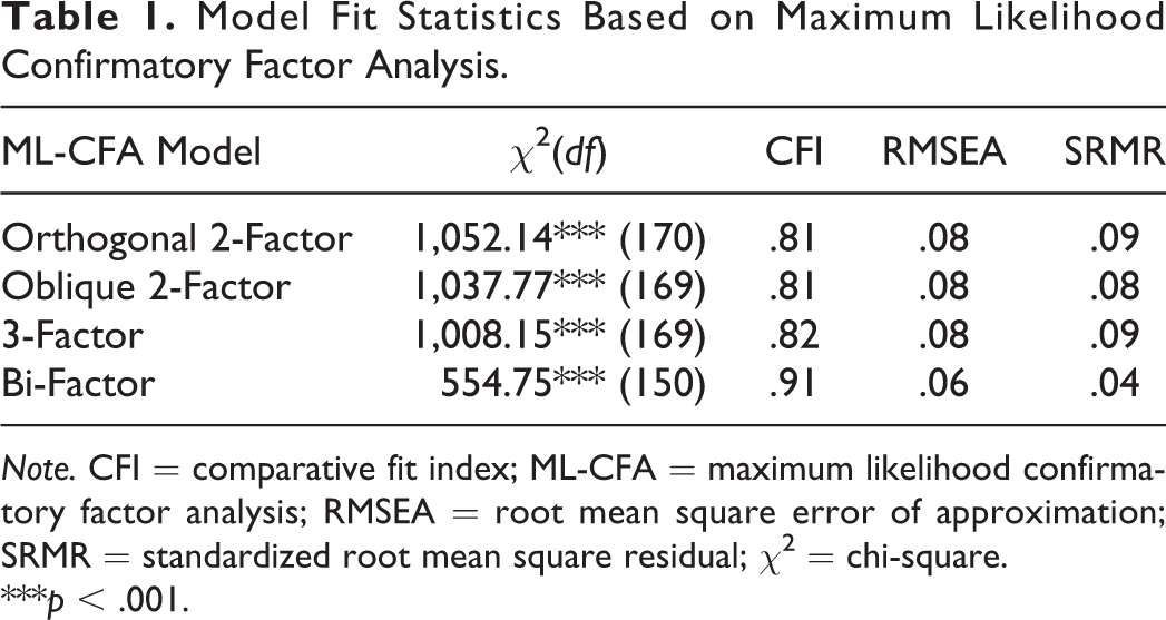
Note. CFI = comparative fit index; ML-CFA = maximum likelihood confirmatory factor analysis; RMSEA = root mean square error of approximation; SRMR = standardized root mean square residual; χ² = chi-square.

***p < .001.

Bayesian Analysis

The PSR values and Kolmogorov–Smirnov test showed that all models converged. The models specifying either (a) noninformative priors or (b) informative priors for cross-loadings using less than 10,000 iterations and models specifying (c) informative priors for both cross-loadings and residual correlations increased the number of iterations to 50,000. Muthén and Asparouhov (2012) recommended that a relatively large number of MCMC iterations be used when estimating complex models such as those that are unidentified and have near zero prior variance. All parameter trace plots showed clear mixing, and all kernel density plots showed smooth distributions, indicating model convergence. Figures 1 and 2 respectively illustrate the trace plot and kernel density plots for the between-item residual covariance of Item 1 (“interested”) and Item 3 (“excited”) in the orthogonal two-factor model as examples.

Figure 1.

Parameter trace plot in the orthogonal two-factor model. Parameter trace plot is shown for the between-item residual covariance of Item 1 (interested) and Item 3 (excited) in the orthogonal 2-factor model.

Figure 2.

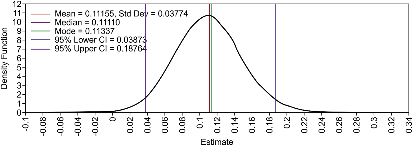
Kernel density plot in the orthogonal two-factor model. Kernel density plot is shown for the between-item residual covariance of Item 1 (interested) and Item 3 (excited) in the orthogonal 2-factor model.

Table 2 summarizes the BSEM results of all investigated models. Model 1(a), an orthogonal two-factor model with noninformative priors, showed a poor model fit with a PPP value of zero and positive 2.5% posterior predictive limit values. Also, given that BRMSEA = 0.08 and the 90% credibility intervals for BRMSEA were above .06, this model did not fit the data even approximately. Essentially, with BCFI = 0.81, BTLI = 0.79, and 90% credibility intervals for the fit indices below .95, we can state with 90% certainty that the model did not fit the data even approximately. Findings for Models 1(b), 2(a), 2(b), and 3(a) were similar in terms of PPP values, positive 2.5% posterior predictive limits, BRMSEA, BCFI, and BTLI; therefore, these models demonstrated a poor model fit as well. Models 3(b), 4(a), and 4(b) showed conflicting results for the model fit index. For all three models, the 2.5% posterior predictive limit was positive and the PPP value was zero. Each model had a BCFI value of about .92 (but less than .95), and the 90% credibility intervals for BCFI were lower than .95. However, regarding BTLI values, those in Models 4(a) and 4(b) were each greater than .95; for Model 3(b), the BCFI was .89. The 90% credibility intervals for the BTLI of Models 4(a) and 4(b) conveyed that these models fit the data well with 90% certainty. In addition, BRMSEA values for all three models were below 0.06. As mentioned earlier, PPP values are sensitive to minor misspecifications whereas BRMSEA is sensitive to major misspecifications. Therefore, models 4(a) and 4(b) required further consideration because the model fit might be acceptable. When specifying informative priors for cross-loadings and residual correlations, all (c) models fit the data well with PPP values of roughly .50 and symmetric posterior predictive limits around zero. With respect to model fit indices, all (c) models had BRMSEA values of less than .06 and 90% credibility intervals above 0.95 for BCFI and BTLI.

Table 2.

Model Fit Based on Bayesian Structural Equation Modeling.

Orthogonal Two-Factor
1a	Noninformative	60	830.96	926.24	.000	.077 (.076, .078)	.809 (.805, .813)	.786 (.781, .790)	50,907.44
1b	Cross-loadings	80	566.92	667.38	.000	.068 (.066, .069)	.867 (.862, .871)	.836 (.830, .841)	50,660.68
1c	Cross-loadings and Residuals	270	-50.14	70.71	.36	.009 (.000, .031)	.999 (.991, 1.00)	.997 (.966, 1.00)	50,157.10
Oblique Two-Factor
2a	Noninformative	61	815.88	912.06	.000	.077 (.076, .078)	.812 (.808, .816)	.789 (.783, .793)	50,894.81
2b	Cross-loadings	81	567.35	666.25	.000	.068 (.067, .069)	.867 (.861, .871)	.835 (.828, .840)	50,662.17
2c	Cross-loadings & Residuals	271	−48.14	71.80	.35	.010 (.000, .032)	.999 (.991, 1.00)	.996 (.964, 1.00)	50,158.62
Three-Factor
3a	Noninformative	61	785.23	883.88	.000	.075 (.075, .076)	.819 (.815, .823)	.796 (.791, .800)	50,864.90
3b	Cross-loadings	101	344.59	454.2	.000	.057 (.055, .059)	.914 (.908, .920)	.885 (.876, .893)	50,454.78
3c	Cross-loadings and Residuals	291	−52.16	66.75	.41	.000 (.000, .029)	1.000 (.992, 1.00)	1.000 (.970, 1.00)	50,153.44
Bi-Factor
4a	Noninformative	80	349.09	451.03	.000	.036 (.035, .037)	.914 (.909, .918)	.953 (.950, .955)	50,249.18
4b	Cross-loadings	100	317.28	419.80	.000	.035 (.034, .036)	.921 (.916, .926)	.956 (.953, .959)	50,222.53
4c	Cross-loadings & Residuals	290	−65.52	52.29	.57	.000 (.000, .010)	1.000 (.995, 1.00)	1.000 (.996, 1.00)	49,951.98

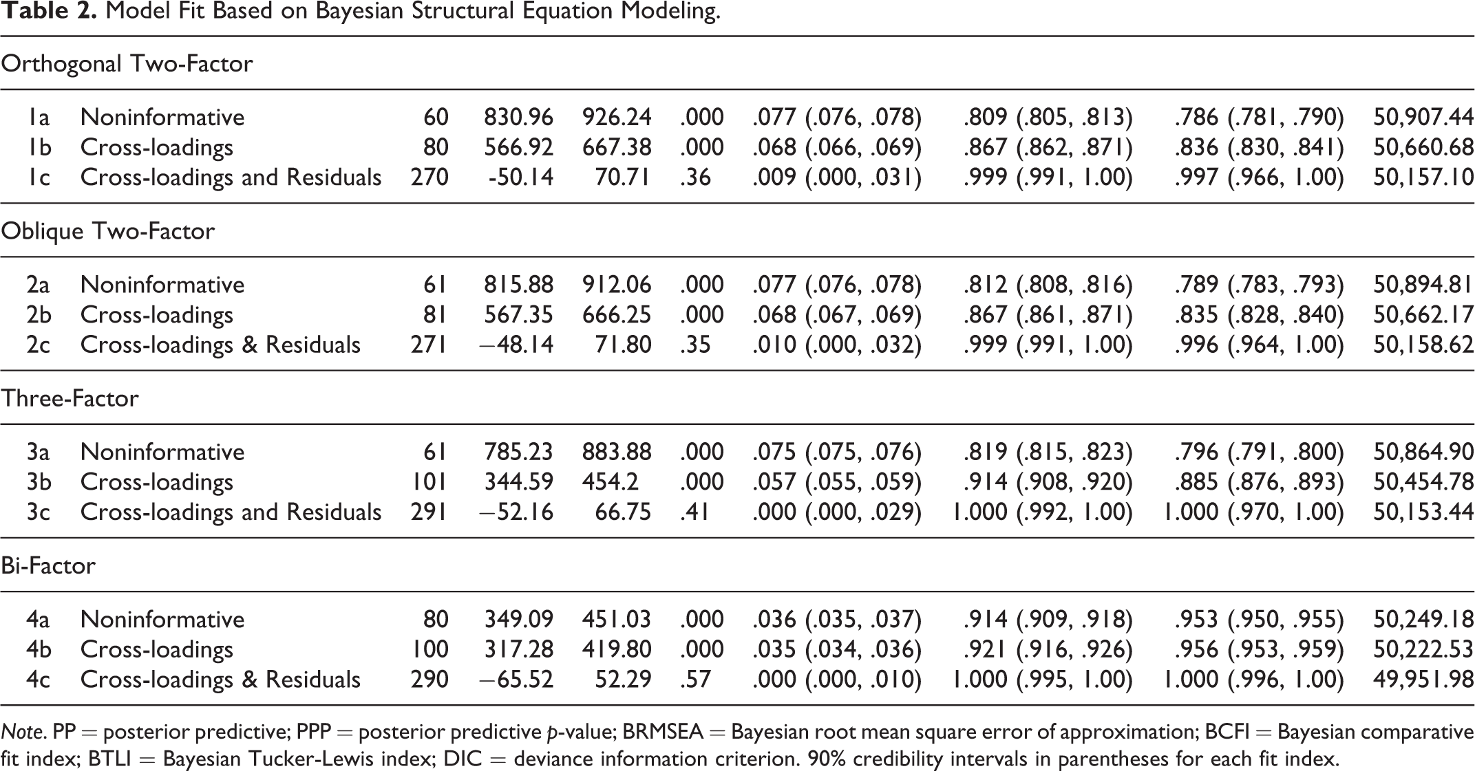
Note. PP = posterior predictive; PPP = posterior predictive p-value; BRMSEA = Bayesian root mean square error of approximation; BCFI = Bayesian comparative fit index; BTLI = Bayesian Tucker-Lewis index; DIC = deviance information criterion. 90% credibility intervals in parentheses for each fit index.

To determine the optimal model, DIC values for the four (c) models and for Models 4(a) and 4(b) were compared. We found that Model 4(c), the bi-factor model with cross-loadings and residual priors, returned the smallest DIC value and differed from the others by more than 200. However, although the bi-factor model fit the data best, differences in DIC values between the two-factor models and three-factor model were negligible (i.e., less than 5). We thus considered the models’ factor loadings, correlations, and parsimony principles more carefully.

In Model 3(c), the three-factor model with cross-loadings and residual priors and that with the second-smallest DIC value, the correlation between AF and UP factors was .99. In other words, items under the AF and UP factors were indistinguishable and did not need to be differentiated. Meanwhile, the oblique two-factor model showed that the correlation between PA and NA factors was negative, small, and non-significant; therefore, based on parsimony, the factors did not need to be correlated. According to correlation and parsimony, the three-factor model and oblique two-factor model were determined to be unsuitable structures for the PANAS.

Factor loadings for the orthogonal two-factor and bi-factor models with cross-loadings and residual priors appear in Table 3. In terms of the orthogonal two-factor model, all items from each scale loaded significantly and positively onto each factor and had substantial values (with the exception of Item 12, the “alert” item). Regarding cross-loadings, Items 1 (“interested”), 3 (“excited”), 19 (“active”), and 20 (“afraid”) showed significantly negative loadings with small values on the opposite factor. These items could thus also function as reverse-scored items. Additionally, Item 12 (“alert”), which originally loaded on the PA factor, significantly and positively loaded on both factors; the size of these factor loadings suggested that loading on the NA scale was more acceptable. For factor loadings in the bi-factor model, we observed that all factor loadings for PA, except Item 12, were much greater than those for AP; that is, items under PA were not explained by AP. Although the bi-factor model demonstrated the relatively best fit to the data, it remained questionable whether the AP factor was appropriate for assessing the PANAS. Also, not all factor loadings for NA were statistically significant; that is, those items were not described for the NA factor in this bi-factor model. Overall, the two-factor orthogonal model was found to have the best fit, with all factor loadings being acceptable. This pattern coincides with findings from Watson et al. (1988).

Table 3.

Factor Loadings From BSEM Orthogonal Two-Factor and Bi-factor Models With Cross-Loadings and Residuals Priors.

Item	PA	NA	PA	NA	PA	NA	AP
Interested (Item 1)	.65	−.15	.65*	−.15*	.63*	−.01	−.24*
Excited (Item 3)	.67	−.11	.68*	−.10*	.66*	.003	−.20*
Strong (Item 5)	.70	.02	.71*	−.04	.71*	−.03	−.06
Enthusiastic (Item 9)	.80	−.01	.81*	−.04	.80*	.004	−.12
Proud (Item 10)	.76	−.06	.76*	−.08	.75*	−.01	−.16*
Alert (Item 12)	.30	.58	.25*	.42*	.30*	.06	.52*
Inspired (Item 14)	.78	.19	.77*	.10	.78*	.02	.07
Determined (Item 16)	.84	.10	.83*	.03	.83*	.01	−.02
Attentive (Item 17)	.67	−.05	.67*	−.07	.67*	.01	−.14*
Active (Item 19)	.71	−.16	.72*	−.14*	.70*	.01	−.25*
Distressed (Item 2)	−.09	.70	−.09	.70*	−.05	−.16	.78*
Upset (Item 4)	−.06	.67	−.07	.67*	−.03	−.10	.72*
Guilty (Item 6)	−.003	.49	−.02	.48*	.001	.09	.47*
Scared (Item 7)	.02	.82	−.02	.82*	.02	.44	.81*
Hostile (Item 8)	.04	.59	.01	.55*	.05	.01	.59*
Irritable (Item 11)	−.08	.77	−.09	.75*	−.05	.07	.79*
Ashamed (Item 13)	.03	.62	.002	.59*	.03	.07	.61*
Nervous (Item 15)	.08	.76	.04	.73*	.07	.20	.72*
Jittery (Item 18)	.12	.57	.08	.55*	.10	.30	.52*
Afraid (Item 20)	−.09	.85	−.12*	.85*	−.08	.47	.85*

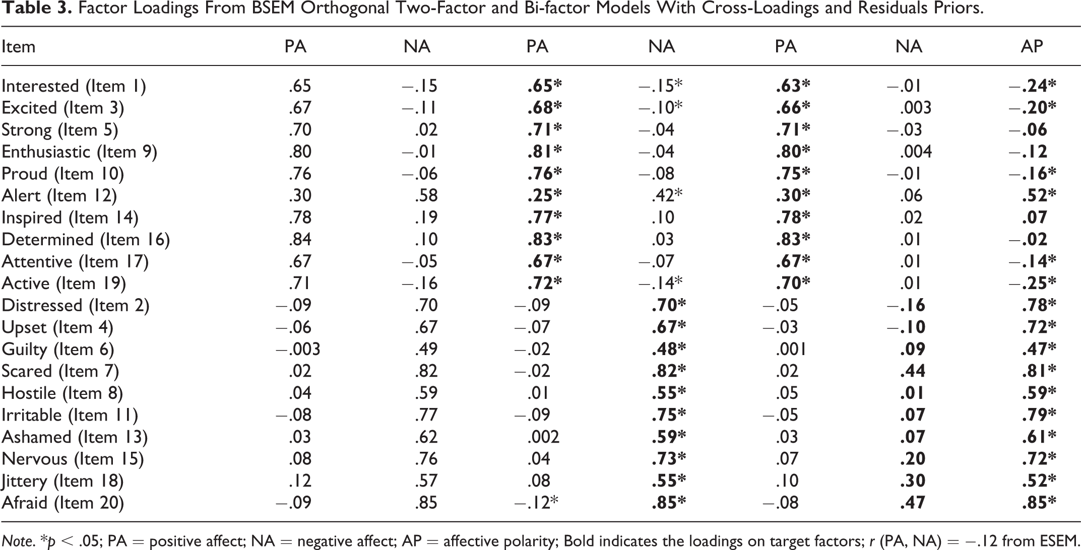
Note. *p < .05; PA = positive affect; NA = negative affect; AP = affective polarity; Bold indicates the loadings on target factors; r (PA, NA) = −.12 from ESEM.

Also for the orthogonal two-factor model, some residual covariances and correlations were statistically significant at the 0.05 level. The correlations among the residuals ranged from −0.12 to 0.21 with a mean of 0.11. Specifically, for the PA items, the correlations between the following residuals were statistically significant: between Items 1 (“interested”) and 3 (“excited”), between Items 3 (“excited”), 14 (“inspired”), 16 (“determined”), and 19 (“active”), and between Items 5 (“strong”), 9 (“enthusiastic”), and 16 (“determined”). In addition, Items 10 (“proud”) and 16 (“determined”), Items 14 (“inspired”) and 16 (“determined”), and Items 16 (“determined”) and 17 (“attentive”) were residually correlated. For the NA items, the residuals of Items 12 (“alert”), 8 (“hostile”) and 13 (“ashamed”) were also correlated. These residual covariances suggest that there are unexplained relations among those items in addition to their shared variances through the common latent factors of PA and NA. One possible explanation for such relations is that the wordings may elicit finer categories of emotions beyond the broad categories of PA and NA (see Cowen & Keltner, 2017). For the NA items, Items 2 (“distressed”), 4 (“upset”), 7 (“scared”), 8 (“hostile”), 11 (“irritable”), 18 (“jittery”), and 20 (“afraid”) were residually correlated. Residual correlations between Items 4 (“upset”), 7 (“scared”), 11 (“irritable”), 18 (“jittery”), and 20 (“afraid”) were statistically significant, as were the residual correlations and between Items 6 (“guilty”), 7 (“scared”), 8 (“hostile”), 13 (“ashamed”), and 15 (“nervous”). Additionally, Items 7 (“scared”) and 20 (“afraid”), Items 8 (“hostile”) and 13 (“ashamed”), Items 15 (“nervous”) and 20 (“afraid”), and Items 18 (“jittery”) and 20 (“afraid”) were statistically significantly correlated.

The BSEM results revealed several potentially beneficial modifications. As such, we re-specified the orthogonal two-factor model using these modifications and analyzed the resultant model with ML-CFA to gauge the improvement in model fit. The new model presented a much better fit than the original: CFI = .97, RMSEA = .03, and SRMR = .04. Moreover, the two-factor model based on BSEM showed a far better fit to the data compared to the two-factor model ESEM solution (CFI = .87, RMSEA = .07, and SRMR = .04). This enhanced fit indicates the merit of BSEM for addressing misspecifications. Notably, the patterns of factor loadings from ESEM were similar to those from BSEM (see Table 3). Detailed modifications suggested by the BSEM results are depicted in Figure 3.

Figure 3.

Respecified orthogonal two-factor model based on BSEM modifications.

Discussion

The main purpose of this study was to identify an appropriate factor model for the PANAS, a measuring instrument used in various domains of psychology such as health and clinical psychology. Clarifying the factor model renders our work comparable to previous studies and can help to ensure more accurate results in subsequent research. Furthermore, we addressed the factor model using BSEM, an emerging method. This manuscript briefly introduced BSEM to outline the approach for researchers who may be less familiar with Bayesian methods.

Through Bayesian estimation, we applied a series of prior specifications across models. An orthogonal two-factor model featuring specified informative priors for cross-loadings and residual correlations was ultimately found to have the best model fit. Consistent with Watson et al.’s (1988) results, all items for each factor loaded statistically significantly and positively on each factor. For the four statistically significantly negative cross-loadings, our analysis indicated that these items may serve as reverse-scored items on the opposite factor. Contrary to our expectation that Item 12 (alert) would load significantly positively on the PA factor only, we found that the direct- and cross-loadings of Item 12 were both significant and positive. This result may have been due to participants’ misunderstanding of the term; although the word “alert” expresses an aspect of positive affect, the word generally implies a negative situation when used as a verb or noun. Thus, many students who participated in this study may have considered this word to represent NA. The term’s meaning should therefore be clarified in subsequent studies, especially those involving younger participants.

The BSEM modification results obtained in this study also revealed strategies for creating a more precise model by re-specifying the ML-CFA model. By applying a frequentist approach, we found that, compared to the original ML factor’s model fit, the re-specified model showed a much better fit. This enhancement highlights the benefit of BSEM modifications. The residual correlations we added based on the final model from our BSEM analysis improved the model fit, suggesting that the BSEM approach can detect model misfit. Future studies may investigate how the model fit relates to the correlated residuals. Another advantage of BSEM modifications is that they can be applied simultaneously rather than sequentially as required by frequentist approaches. This option is appealing because it can save time and effort when modifying the model.

In this study, ESEM procedures were briefly implemented and compared to final models to examine the factor structure of the PANAS. ESEM has been proposed to address similar limitations associated with CFA and EFA, much like BSEM (Asparouhov & Muthén, 2009). However, ESEM that relies on frequentist statistics and inferences and BSEM that is based on a Bayesian approach differ in two major ways. First, ESEM is more data-driven: in an ESEM model, the researcher does not specify which items have high (and low) loadings; instead, all items load on all factors as in EFA, and these “exploratory” factors can affect other (latent or observed) variables. Typically, the focus is on the relationships between these exploratory factors and other variables rather than on exploratory factors themselves. BSEM, similar to other Bayesian-based models, is more theory-driven and typically starts with a researcher’s hypothesis regarding the factor structure. Second, ESEM, like EFA, suffers from an indeterminacy problem in that an infinite number of sets of parameter estimates can be created for the same analysis(Gorsuch, 1988; Grice, 2001). This problem can result in misaligned factors in multi-group analysis (e.g., the first factor in Group 1 may be the second factor in Group 2). On the contrary, factors identified via BSEM are unambiguously represented in the model. In other words, BSEM, which can take into account the factor loadings and variance of non-targeted factors, can identify only one solution based on the researcher’s hypothesis. BSEM can thus be easily extended to multi-group analysis.

Studies on affects, emotions, feelings, and moods are fundamentally interesting to researchers in psychology in general and to those in health psychology in particular. While there are differences among these terms (Tyng et al., 2017), it has shown that such emotional experiences by people can affect cognitive functions. Emotional health is associated with success in work, relationships, and physical health; specific emotions may lead to different health outcomes (Consedine & Moskowitz, 2007). Our findings that the two-factor orthogonal model was the best among all models investigated suggest there might be a hierarchy of affects and emotions. Future research could look into emotional experiences that are not captured by the PANAS.

While this study supports the original factor structure of the PANAS using a new approach, there are limitations. First, data were only collected from a single province in mainland China. This constraint led to sample homogeneity and limited the generalizability of our findings. Data from other samples are warranted for the factor structure of the PANAS. Second, participants in this study were all adolescents, and some might have struggled to understand certain items. Laurent et al. (1999) developed the PANAS-C specifically for children, and this instrument may have been a better choice for our study than the PANAS. Third, our analysis did not consider participant characteristics, such as gender and whether a student was an only child. The only-child variable is a unique cultural artifact related to China’s one-child policy. Because only children are likely to receive more attention from their parents than children with siblings, participants’ responses and the effect of PA or NA could presumably vary between only children and those with siblings. Although many studies have focused on personality-related differences between these groups, results have been inconsistent (Wang & Guo, 2017). For the gender variable, applying a multiple-indicator multiple-cause model may be worthwhile. Although scholars have analyzed gender differences using factorial invariance, findings have been limited, ambiguous, and occasionally contradictory (Crawford & Henry, 2004; Merz et al., 2013). Finally, it would be interesting to adopt a different version of the PANAS to validate the instrument in subsequent studies. Most existing work has investigated the factor structure of the original PANAS or short forms of the schedule (Merz et al., 2013). Examining the structure of other PANAS versions via BSEM would provide additional insight and reinforce the instrument’s structural validity.

Supplemental Material

Supplemental Material, sj-pdf-1-ehp-10.1177_0163278721996794 - Factor Structure of the PANAS With Bayesian Structural Equation Modeling in a Chinese Sample

Supplemental Material, sj-pdf-1-ehp-10.1177_0163278721996794 for Factor Structure of the PANAS With Bayesian Structural Equation Modeling in a Chinese Sample by Minsun Kim and Ze Wang in Evaluation & the Health Professions

Footnotes

Declaration of Conflicting Interests

The author(s) declared no potential conflicts of interest with respect to the research, authorship, and/or publication of this article.

Funding

The author(s) received no financial support for the research, authorship, and/or publication of this article.

ORCID iDs

Minsun Kim

Ze Wang

Supplemental Material

Supplemental material for this article is available online.

References

Asparouhov

Muthén

(2009). Exploratory structural equation modeling. Structural Equation Modeling: A Multidisciplinary Journal, 16(3), 397–438. https://doi.org/10.1080/10705510903008204

Asparouhov

Muthén

(2010). Bayesian analysis of latent variable models using Mplus. Version 4. Retrieved from http://www.statmodel.com/download/BayesAdvantages18.pdf

Asparouhov

Muthén

Morin

A. J. S.

(2015). Bayesian structural equation modeling with cross-loadings and residual covariances: Comments on Stromeyer et al. Journal of Management, 41(6), 1561–1577. https://doi.org/10.1177/0149206315591075

Beck

J. G.

Novy

D. M.

Diefenbach

G. J.

Stanley

M. A.

Averill

P. M.

Swann

A. C.

(2003). Differentiating anxiety and depression in older adults with generalized anxiety disorder. Psychological Assessment, 15(2), 184–192. https://doi.org/10.1037/1040-3590.15.2.184

Berger

(2006). The case for objective Bayesian analysis. Bayesian Analysis, 1(3), 385–402. https://doi.org/10.1214/06-BA115

Can

van de Schoot

Hox

(2015). Collinear latent variables in multilevel confirmatory factor analysis: A comparison of maximum likelihood and Bayesian estimation. Educational and Psychological Measurement, 75, 406–427. https://doi.org/10.1177/0013164414547959

Chen

F. F.

West

S. G.

Sousa

K. H.

(2006). A Comparison of Bifactor and Second-Order Models of Quality of Life. Multivariate Behavioral Research, 41(2), 189–225. https://doi.org/10.1207/s15327906mbr4102_5

Chung

P. K.

Dong Liu

(2012). Examination of the psychometric properties of the Chinese translated behavioral regulation in exercise questionnaire-2. Measurement in Physical Education and Exercise Science, 16(4), 300–315. https://doi.org/10.1080/1091367X.2012.693364

Consedine

N. S.

Moskowitz

J. T.

(2007, November 1). The role of discrete emotions in health outcomes: A critical review. Applied and Preventive Psychology, 12(2), 59–75. https://doi.org/10.1016/j.appsy.2007.09.001

10.

Cowen

A. S.

Keltner

(2017). Self-report captures 27 distinct categories of emotion bridged by continuous gradients. Proceedings of the National Academy of Sciences, 114(38), E7900–E7909. https://doi.org/10.1073/pnas.1702247114

11.

Crawford

J. R.

Henry

J. D.

(2004). The positive and negative affect schedule (PANAS): Construct validity, measurement properties and normative data in a large non-clinical sample. British Journal of Clinical Psychology, 43, 245–265. https://doi.org/10.1348/0144665031752934

12.

Crocker

P. R. E.

(1997). A confirmatory factor analysis of the positive affect negative affect schedule (PANAS) with a youth sport sample. Journal of Sport and Exercise Psychology, 19(1), 91–97. https://doi.org/10.1123/jsep.19.1.91

13.

De Beer

L. T.

Van Zyl

L. E.

(2019). ESEM code generator for Mplus. https://www.surveyhost.co.za/esem/ https://doi:10.6084/m9.figshare.8320250

14.

Garnier-Villarreal

Jorgensen

T. D.

(2020). Adapting fit indices for Bayesian structural equation modeling: Comparison to maximum likelihood. Psychological Methods, 25(1), 46–70. https://doi.org/10.1037/met0000224

15.

Gaudreau

Sánchez

Blondin

(2006). Positive and negative affective states in a performance-related setting: Testing the factorial structure of the PANAS across two samples of French-Canadian participants. European Journal of Psychological Assessment, 22, 240–249. https://doi.org/10.1027/1015-5759.22.4.240

16.

Gelman

Carlin

J. B.

Stern

H. S.

Dunson

D. B.

Vehtari

Rubin

D. B.

(2014). Bayesian data analysis (3rd ed.). CRC Press.

17.

Gorsuch

R. L.

(1988). Exploratory factor analysis. In Nesselroade

J. R.

Cattell

R. B.

(Eds.), Handbook of multivariate experimental psychology (pp. 231–258). Springer US. https://doi.org/10.1007/978-1-4613-0893-5_6

18.

Grice

J. W

., (2001). Computing and evaluating factor scores. Psychological Methods, 6, 430–450. https://doi.org/10.1037//1082-989X.6.4.430-450

19.

Harring

J. R.

Weiss

B. A.

Hsu

J.-C.

(2012). A comparison of methods for estimating quadratic effects in nonlinear structural equation models. Psychological Methods, 17(2), 193–214. https://doi.org/10.1037/a0027539

20.

Hoofs

van de Schoot

Jansen

N. W. H.

Kant

(2018). Evaluating model fit in Bayesian confirmatory factor analysis with large samples: Simulation study introducing the BRMSEA. Educational Psychological Measurement, 78(4), 537–568. https://doi.org/10.1177/0013164417709314

21.

L. T.

Bentler

P. M.

(1999). Cutoff criteria for fit indexes in covariance structure analysis: Conventional criteria versus new alternatives. Structural Equation Modeling: A Multidisciplinary Journal, 6(1), 1–55. https://doi.org/10.1080/10705519909540118

22.

Jovanović

Gavrilov-Jerković

(2016). The structure of adolescent affective well-being: The case of the PANAS among Serbian adolescents. Journal of Happiness Studies, 17(5), 2097–2117. https://doi.org/10.1007/s10902-015-9687-8

23.

Kaplan

Depaoli

(2012). Bayesian structural equation modeling. In Hoyle

R. H.

(Ed.), Handbook of structural equation modeling (pp. 650–673). The Guilford Press.

24.

Kaplan

Depaoli

(2013). Bayesian statistical methods. In Little

T. D.

(Ed.), The Oxford handbook of quantitative methods (Vol. 1): Foundations (pp. 407–437). Oxford University Press.

25.

Kercher

(1992). Assessing subjective well-being in the old-old: The PANAS as a measure of orthogonal dimensions of positive and negative affect. Research on Aging, 14(2), 131–168. https://doi.org/10.1177/0164027592142001

26.

Killgore

W. D. S.

(2000). Evidence for a third factor on the positive and negative affect schedule in a college student sample. Perceptual and Motor Skills, 90(1), 147–152. https://doi.org/10.2466/pms.2000.90.1.147

27.

Kohli

Hughes

Wang

Zopluoglu

Davison

M. L.

(2015). Fitting a linear–linear piecewise growth mixture model with unknown knots: A comparison of two common approaches to inference. Psychological Methods, 20(2), 259–275. https://doi.org/10.1037/met0000034

28.

Krohne

H. W.

Egloff

Kohlmann

C.-W.

Tausch

(1996). Untersuchungen mit einer deutschen Version der “Positive and Negative Affect Schedule” (PANAS) [Investigations with a German version of the Positive and Negative Affect Schedule (PANAS)]. Diagnostica, 42(2), 139–156.

29.

Laurent

Catanzaro

S. J.

Joiner

T. E.

Jr Rudolph

K. D.

Potter

K. I.

Lambert

Osborne

Gathright

(1999). A measure of positive and negative affect for children: Scale development and preliminary validation. Psychological Assessment, 11(3), 326–338. https://doi.org/10.1037/1040-3590.11.3.326

30.

Lee

S.-Y.

(2007). Structural equation modeling: A Bayesian approach. John Wiley & Sons.

31.

Leue

Beauducel

(2011). The PANAS structure revisited: On the validity of a bifactor model in community and forensic samples. Psychological Assessment, 23(1), 215–225. https://doi.org/10.1037/a0021400

32.

Lüdtke

Marsh

H. W.

Robitzsch

Trautwein

(2011). A 2 × 2 taxonomy of multilevel latent contextual models: Accuracy–bias trade-offs in full and partial error correction models. Psychological Methods, 16(4), 444–467. https://doi.org/10.1037/a0024376

33.

Mackinnon

Jorm

A. F.

Christensen

Korten

A. E.

Jacomb

P. A.

Rodgers

(1999). A short form of the positive and negative affect schedule: Evaluation of factorial validity and invariance across demographic variables in a community sample. Personality and Individual Differences, 27(3), 405–416. https://doi.org/10.1016/S0191-8869(98)00251-7

34.

Marsh

H. W.

Ludtke

Muthén

Asparouhov

Morin

A. J.

Trautwein

Nagengast

(2010). A new look at the big five factor structure through exploratory structural equation modeling. Psychological Assessment, 22(3), 471–491. https://doi.org/10.1037/a0019227

35.

Marsh

H. W.

Morin

A. J. S.

Parker

P. D.

Kaur

(2014). Exploratory structural equation modeling: an integration of the best features of exploratory and confirmatory factor analysis. Annual Review of Clinical Psychology, 10(1), 85–110. https://doi.org/10.1146/annurev-clinpsy-032813-153700

36.

Marsh

H. W.

Muthén

Asparouhov

Lüdtke

Robitzsch

Morin

A. J. S.

Trautwein

(2009). Exploratory structural equation modeling, integrating CFA and EFA: Application to students’ evaluations of university teaching. Structural Equation Modeling: A Multidisciplinary Journal, 16(3), 439–476. https://doi.org/10.1080/10705510903008220

37.

Mehrabian

(1997). Comparison of the PAD and PANAS as models for describing emotions and for differentiating anxiety from depression. Journal of Psychopathology and Behavioral Assessment, 19(4), 331–357. https://doi.org/10.1007/BF02229025

38.

Melvin

G. A.

Molloy

G. N.

(2000). Some psychometric properties of the positive and negative affect schedule among Australian youth. Psychological Reports, 86(3). https://doi.org/10.2466/pr0.2000.86.3c.1209

39.

Merz

E. L.

Malcarne

V. L.

Roesch

S. C.

C. M.

Emerson

Roma

V. G.

Sadler

G. R.

(2013). Psychometric properties of positive and negative affect schedule (PANAS) original and short forms in an African American community sample. Journal of Affective Disorders, 151(3), 942–949. https://doi.org/10.1016/j.jad.2013.08.011

40.

Muthén

Asparouhov

(2012). Bayesian structural equation modeling: A more flexible representation of substantive theory. Psychological Methods, 17(3), 313–335. https://doi.org/10.1037/a0026802

41.

Muthén

L. K.

Muthén

B. O.

(2017). Mplus User's Guide. (8th ed.). Los Angeles, CA: Muthén & Muthén.

42.

Schoot

Kaplan

Denissen

Asendorpf

Neyer

Aken

(2013). A Gentle introduction to Bayesian analysis: Applications to developmental research. Child Development, 85. https://doi.org/10.1111/cdev.12169

43.

Seib-Pfeifer

L.-E.

Pugnaghi

Beauducel

Leue

(2017). On the replication of factor structures of the positive and negative affect schedule (PANAS). Personality and Individual Differences, 107, 201–207. https://doi.org/10.1016/j.paid.2016.11.053

44.

Serafini

Malin-Mayor

Nich

Hunkele

Carroll

K. M.

(2016). Psychometric properties of the positive and negative affect schedule (PANAS) in a heterogeneous sample of substance users. The American Journal of Drug and Alcohol Abuse, 42(2), 203–212. https://doi.org/10.3109/00952990.2015.1133632

45.

Shi

Wang

(2009). Age-related change in emotional experience in a sample of Chinese adults: A preliminary study. Psychological Reports, 105(1), 37–42. https://doi.org/10.2466/pr0.105.1.37-42

46.

Thompson

E. R.

(2007). Development and validation of an internationally reliable short-form of the positive and negative affect schedule (PANAS). Journal of Cross-Cultural Psychology, 38(2), 227–242. https://doi.org/10.1177/0022022106297301

47.

Tyng

C. M.

Amin

H. U.

Saad

M. N. M.

Malik

A. S.

(2017, August 24). The influences of emotion on learning and memory [Review]. Frontiers in Psychology, 8(1454). https://doi.org/10.3389/fpsyg.2017.01454

48.

Vera-Villarroel

Celis-Atenas

Urzúa

Jaime

Contreras

Lillo

Zych

Silva

J. R.

(2019). Positive and negative affect schedule (PANAS): Psychometric properties and discriminative capacity in several Chilean samples. Evaluation and the Health Professions, 42(4), 473–497. https://doi.org/10.1177/0163278717745344

49.

Villodas

M. T.

Roesch

(2017). Examining the factor structure of the positive and negative affect schedule (PANAS) in a multiethnic sample of adolescents. Measurement and Evaluation in Counseling and Development, 44(4), 193–203. https://doi.org/10.1177/0748175611414721

50.

Wang

Guo

Y. Y.

(2017). Deriving a structural model for the multidimensional self- concept construct: A case of middle school students in mainland China. In Williams

(Ed.), Self-Concept perceptions cultural differences and gender differences (pp. 77–106). Nova Publishers.

51.

Watson

Clark

L. A.

(1994). The PANAS-X: Manual for the positive and negative affect schedule—expanded form. University of Iowa.

52.

Watson

Clark

L. A.

Tellegen

(1988). Development and validation of brief measures of positive and negative affect: The PANAS scales. Journal of Personality and Social Psychology, 54(6), 1063–1070. https://doi.org/10.1037//0022-3514.54.6.1063

53.

Weidong

Jing

Schick

C. J.

(2004). The cross-cultural measurement of positive and negative affect examining the dimensionality of PANAS. Psychological Science (China), 27(1), 77–79.

Supplementary Material

Please find the following supplemental material available below.

For Open Access articles published under a Creative Commons License, all supplemental material carries the same license as the article it is associated with.

For non-Open Access articles published, all supplemental material carries a non-exclusive license, and permission requests for re-use of supplemental material or any part of supplemental material shall be sent directly to the copyright owner as specified in the copyright notice associated with the article.

0.00 MB

0.01 MB