Health Status,Health Shocks,and Asset Adequacy Over Retirement Years

Abstract

This article uses data on a sample of retirees drawn from the Health and Retirement Study (HRS) to examine changes in health over the retirement years and to estimate the effects of health changes in retirement on wealth. Using the framework of item response theory, we develop a novel measure of health that makes use of multiple indicators of physical health that are available in the HRS. We find that large negative shocks to the health of male retirees and their spouses are frequent in retirement and that when such shocks do occur, recovery to the preshock level of health is rare. Using a dynamic panel data model, we then estimate short- and long-run effects of changes in health on wealth. While our estimated short-run effects are modest, long-run estimates of the impact of health shocks on wealth are large, ranging from a 12% to 20% reduction in wealth by the 10th year, following a permanent one standard deviation decrease in health.

Keywords

health measurement health shocks wealth effects item response theory

While individuals entering retirement may have sufficient financial, housing, and pension assets at the time of retirement, they may have difficulty maintaining this position because of unexpected negative changes in health status, real estate and financial equity prices, and public retirement and health-care programs. Here, we explore the role of health and health changes or shocks on retiree’s assets, focusing on both the likelihood of such shocks and the resulting changes in financial resources. Using a sample of retirees drawn from the Health and Retirement Study (HRS), we employ an econometric model developed for dynamic panel data with household effects and also present a novel and comprehensive measure of physical health constructed using item response theory (IRT).

Using our IRT-based measure of physical health status, we are able to advance knowledge regarding the health-related threats to economic independence for older citizens. In particular, we (1) focus exclusively on a sample of individuals who have actually retired,¹ (2) study longer term consequences of health shocks following retirement, (3) address issues that are important to understand a variety of effects of policy reform, and (4) analyze the effect of shocks on wealth, defined as the sum of financial, business, and housing wealth.²

Review of Prior Literature

This research builds on several ongoing lines of research, including studies pertaining to the measurement of health status, and the impact of health shocks on wealth and a variety of behaviors (e.g., work, asset allocation, and consumption).

The Adequacy of Resources in Retirement

Numerous research articles have examined the adequacy of resources in retirement; they differ significantly in the data used, research methods, and conclusions. Much of the research on the adequacy of resources in retirement assesses the extent to which preretirement savings behavior of those close to retirement is sufficient to ensure adequate retirement resources (Bernheim, 1992; Moore and Mitchell, 2000; Butrica, Iams and Smith, 2003, 2007; Gustman and Steinmeier, 1998; Engen, Gale and Uccello, 1999; Wolff, 2002; Haveman, Holden, Romanov and Wolfe, 2007a, 2007b; Haveman, Holden, Wolfe and Sherlund, 2006; Mitchell, Moore and Phillips, 2000; and Scholz, Sheshadri and Khitatrakun, 2006). The methods of these assessments vary substantially from comparisons of expected income or annuitized wealth to a poverty threshold (Haveman, Holden, Romanov, & Wolfe, 2007a, 2007b; Haveman, Holden, Wolfe, & Sherlund, 2006; Wolff, 2002) to comparisons between actual savings and optimal savings trajectories derived from dynamic stochastic utility-based models (Engen, Gale, & Uccello, 1999; Scholz, Sheshadri, & Khitatrakun, 2006). Given the differing methods and criteria employed, results on resource adequacy differ substantially, with some studies finding relatively high average rates of savings adequacy (e.g., Scholz et al., 2006) and others finding modest to substantial shortfalls in savings (e.g., Haveman et al., 2007a, 2007b; Wolff, 2002).

Measurement of Health Status

Many studies of the role of health use the five-response subjective general health measure.³ Other studies, especially those by epidemiologists, use a set of variables that include particular illness or injuries, deaths, hospitalizations, and days of work or school lost. Other analyses combine information about various health conditions to estimate health-adjusted life years or the number of healthy years an individual is expected to live.⁴ A committee established by the Institute of Medicine suggests that no one of the approaches studied dominates all others in terms of consistency (Committee to Evaluate Measures of Health Benefits for Environmental, Health, and Safety Regulation, Board on Health Care Services, Institute of Medicine, 2006).

Health, Health Shocks, and Wealth

Several studies provide evidence on how wealth and its components (in particular, individual retirement accounts and 401(k) pensions and housing wealth as forms of self-insurance) evolve during retirement (Coile and Milligan, 2009; Haveman et al., 2007a, 2007b; Holden and Schrass, 2015; Megbolugbe, Sa-Aadu and Shilling, 1997, 1999; Poterba, Venti and Wise, 2011; Venti and Wise, 2002, 2004; Wallace, Haveman, Holden and Wolfe, 2010, 2013).

Studies that report on the effect of health and health shocks on wealth use a variety of data, adopt numerous estimation strategies, and employ varying concepts of both wealth and health shocks (Smith, 1999; Coile and Milligan, 2009; Poterba et al., 2011; and Wallace et al., 2010, 2013). All find sizable negative effects of health shocks on assets. In this article, we examine a set of questions related to those in the prior literature, using a comprehensive measure of financial and housing wealth, a particular sampling frame, a comprehensive measure of health, and a unique empirical methodology.

Data

We use data drawn from the initial cohort of the HRS.⁵ Our analysis sample consists of HRS cohort households that entered retirement as married coupled households, which we define around a male retiree. “Retirement” occurs when the male householder reports receipt of Social Security or Social Security Disability Insurance (SSDI) benefits. Households are tracked from the time they enter retirement until the male retiree dies, attrites from the sample, or when information available from the panel expires. We continue to track male retired households regardless of any changes in household composition due to the death of the retiree’s spouse, divorce, or subsequent remarriage following widowerhood or divorce.⁶

Measuring Wealth and Components

For each wave in which a household is observed, we obtain the value of components of total wealth reported directly by the household-designated “financial respondent.”⁷

Table 1 shows mean total wealth for the households in our sample, along with wealth components during the first-wave postretirement. Mean total wealth is about US$523,000; of that total, US$149,000 is mean housing wealth. Nonhousing wealth is largely composed of financial wealth and is the only wealth component that is readily available for use in the short term; its mean value is US$374,000.

Table 1.

Means and Standard Deviations (First Wave of Retirement, Thousands of 2010 Dollars).

Variable	Mean	SD
Total wealth	523.30	917.82
Housing wealth	149.39	168.91
Nonhousing wealth	374.43	810.45
Retiree’s age	64.49	2.07
Spouse’s age	60.41	5.18
Health measures
Retiree’s health score	0.00	1.00
Spouse’s health score	−0.12	0.98
Spouse’s health score missing (=1)	0.02	0.15
Education level
Less than high school	0.24	0.42
High school	0.36	0.48
Some college	0.18	0.39
College degree	0.22	0.41
Race
White	0.82	0.39
Black	0.09	0.29
Hispanic	0.08	0.27
Asian	0.01	0.11
Number of waves	4.93	2.36

Note. Data used in estimation are from the Rand version of the Health and Retirement Study and include cohort respondents, ages 53–62 in 1994; see description of sample in the third section.

Measuring Health

The HRS contains detailed information on a wide range of health status indicators, including respondent assessments of health (on a 5-point scale). There are also respondent reports on functional limitations, health behaviors (alcohol and tobacco usage), activity levels, height, weight, and physician-diagnosed chronic conditions (e.g., heart disease, cancer, diabetes, and arthritis).

From our prior work (Wallace, Haveman, Holden, & Wolfe, 2010, 2013), we conclude that a reliable assessment of the effect of health shocks on economic status (wealth and wealth adequacy) requires the construction of a composite health measure that incorporates a broad range of information on health status and reflects the transitory nature of retiree health status. We develop a measure of latent physical health status based on IRT, a framework for confirmatory factor analysis in the context of items that have discrete responses and are related to a unidimensional latent trait.⁸

In the IRT framework, responses to a particular item are modeled with an item response function that links the value of the latent health trait to a probability of an affirmative response to the item. Key features of an item’s response function include its difficulty and its ability to discriminate amongst individuals with different values of the latent trait.⁹ IRT models require estimating common parameters of the item characteristics function by way of marginal maximum likelihood.¹⁰ These parameter estimates, along with the pattern of responses to the items, can then be used to estimate the value of the latent trait for each individual that responded to some subset of the items in the test.

Using the IRT framework, we constructed a physical health score using responses to 21 items available in the HRS for each wave between 1994 and 2010.¹¹ Our score is constructed on a standard normal scale with respect to male retirees in the first postretirement wave. Higher scores indicate better health.

One advantage of utilizing an IRT-based approach is that health scores can be estimated for respondents who provide answers to any subset of the 21 items. Another principle advantage of score measures constructed on the basis of the IRT framework is that it provides feedback on the measure’s strengths and weaknesses. In particular, standard errors for each respondent in each wave vary by health score and also response patterns, including nonresponse to one or more items. For our particular measure, standard errors are smallest for health scores in the range of −2 to −1 and are highest for health scores above 0.5. Thus, our measure is most reliable for individuals who are in moderately poor health and is less reliable for individuals in good or better than good health.

One way to gauge the quality of our health measure is to assess the extent to which the health measure is related to health conditions that were not used in its construction and subsequent mortality. Figure 1 shows the percentage of respondents who ever had physician-diagnosed chronic conditions (heart disease, lung disease, high blood pressure, cancer, stroke, and diabetes), who have died by Wave 10 (2010), and average out-of-pocket medical expenses by their health score quintile in 1994 (Wave 2). Information on these conditions was not used in the construction of our health measure. Our constructed scores are quite predictive of the chronic conditions with the exception of cancer, and are also predictive of subsequent mortality and out-of-pocket medical expenses.¹²

Figure 1.

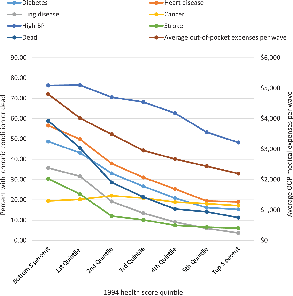
Percentage with chronic conditions or dead by 2010 and average out-of-pocket medical expenses per wave by 1994 Health Score Quintile (Health and Retirement Study cohort respondents ages 53–62 in 1994).

Health in Retirement

Panels A and B of Figure 2 show the average health score of male retirees and spouses by postretirement wave. Figure 2 also shows the cumulative percentage of retirees and spouses who have died and mortality-adjusted health scores. In constructing this adjustment for selection on mortality, we ascribe the last observed health score prior to death to those retirees and spouses who are deceased. This adjustment results in average health profiles that are more sharply decreasing in waves postretirement. For male retirees, mortality-adjusted health scores decrease by about 0.92 standard deviations (SDs) over the retirement period. For spouses, who start out less healthy but are modally younger, the decrease is smaller at about 0.7 SDs of first retirement wave retiree health.

Figure 2.

Average standardized health scores by postretirement wave.

Figure 3 provides some basic descriptive information on the evolution of health after retirement by showing the wave-specific mortality-adjusted average health scores by health score quintile in the first postretirement wave for male retirees (Panel A) and their spouses (Panel B).¹³ During the first-wave postretirement, there are rather large differences in health scores with retirees (spouses) in the top quintile of the health score distribution having an average score of nearly 1.3 (1.1) compared to those in the bottom quintile that have an average score of −1.6. With few exceptions, average health scores within each of the first retirement wave quintiles decrease through the retirement years with larger declines for those in the upper quintile of health and very modest ones for those in the bottom quintile. The net result of this pattern is that the differences in health scores by health score quintile decrease over retirement duration.

Figure 3.

Average standardized health scores by first postretirement wave health score quintile (mortality adjusted).

We turn next to changes in standardized health scores for individuals by examining the cumulative likelihood of one SD decrease in health. Figure 4 shows estimates of the cumulative probability of a one SD wave-to-wave decrease in health (Panel A) and a one SD decrease in health measured from the first postretirement wave (Panel B) for male retirees and their spouses.¹⁴ One SD decreases in health are quite common; for example, such changes occur for about 30% of retirees and spouses by the fifth-wave postretirement. The likelihood of large health declines differ substantially across the distribution of postretirement health, with those who retire in better health facing a higher likelihood of a large health decline.¹⁵

Figure 4.

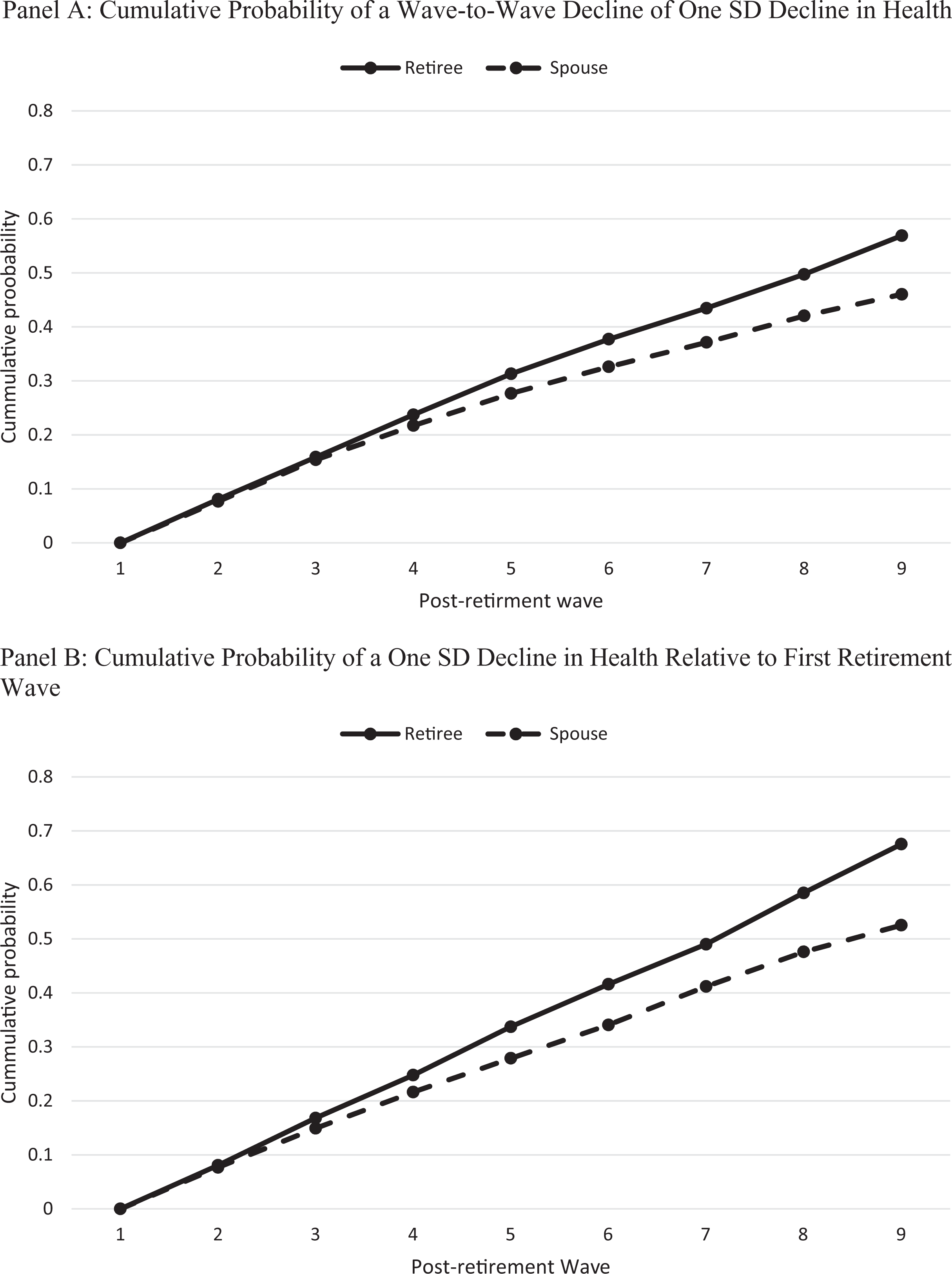
Cumulative probability of a one standard deviation decline in health.

What type of health-related changes are associated with a one SD decrease in health scores?¹⁶ The modal pattern of item response for respondents with a wave-to-wave decline of health of one SD is to report difficulty jogging 1 mile, no difficulty with any other items, and self-reported health of “very good” when they previously reported no difficulty with any items and self-reported health of “excellent.” Although the pattern of responses described above is the most frequently occurring among respondents with a wave-to-wave health decline of one SD or more, it accounts for only slightly more than 4% of such cases. The other patterns of item response declines in health are quite varied and difficult to simplify into a set of patterns.¹⁷

To what extent do large wave-to-wave health score decreases correspond to permanent versus transitory changes in health? We attempt to answer this question by examining the distribution of one, two, and three waves forward health changes following a wave-to-wave standardized health score decline of greater than 1. Within the set of cases that we observe, full recovery from large wave-to-wave health score declines is rare and death following large health score declines is quite common. Overall, 6.2% of male retirees and 7.3% of female spouses with observable forward health outcomes bounce back from health score declines of one SD or more in the first period following the decline. By comparison, nearly 14% of respondents and 9% of spouses with observable health outcomes died in the wave following their health score decline, and over 24% of these respondents and 13% of spouses died within three waves of their health score decline.

In sum, health changes during retirement are rather dramatic. On average, accounting for the effects of mortality, scores decline by nearly one SD over the period that we observe these retirees. There are dramatic differences in the health of retirees at retirement, but these differences partially dissipate over time as individuals who entered retirement in relatively good health experience larger declines throughout retirement. Finally, large declines in health scores are quite common with wave-to-wave and relative to baseline declines of one SD occurring for about one third of all retirees and their spouses by the fifth postretirement wave. When large wave-to-wave declines in health occur, they tend to be permanent in the sense that recovery to the previously observed level of health is rare while death is common.

Method

Conceptually, our model of the evolution of wave-to-wave postretirement wealth is described by the following equation:

{wealth}_{t + 1} = (1 + r) \cdot [{wealth}_{t} - C_{t} {({wealth}_{t}, {health}_{t})}_{t}]

where wealth_t is the wealth in the first period, r is the 2-year rate of return on the current stock of wealth, and C()_t represents consumption between period t and period t + 1, which may be a function of the stock of wealth in period t as well as health status between periods t and t + 1. With this framework, a negative shock to health will have an immediate effect on wealth through its effect on consumption but may also have a larger longer run effect, as the shock-reduced wealth in period t + 1 implies lower future absolute returns.

Based on this conceptual model, we posit the following reduced form equation for the evolution of wealth postretirement:

\ln ({wealth}_{i t}) = α \cdot \ln ({wealth}_{i t - 1}) + β' {health}_{i t} + η' f_{i} + γ' x_{i t} + v_{i t} .

In Equation 1, wealth_it is household i's log wealth in retirement period t, health_it is a vector containing the standardized health scores of the retiree and female spouse, f_i is a vector of household-level, time-invariant characteristics, x_it is a vector of household-level, time-variant characteristics, and v_it = θ_i + ∊_it is an error term with components consisting of an individual effect θ_i and an independent and identically distributed error term ∊_it. Treating θ_i as a fixed effect in Equation 1 and estimating via ordinary least square (OLS) will result in downward biased and inconsistent estimates of α in short panels (Nickell, 1981). Moreover, estimating by OLS without an individual-level error component (θ_i) or treating θ_i as a random effect will result in upward biased and inconsistent estimates of α because θ_i is positively correlated with wealth_{it − 1} by construction.

To provide consistent and unbiased estimates of the parameters of Equation 1, we utilize a generalized method of moments (GMM) estimator proposed by Arellano and Bover (1995) and developed more fully by Blundell and Bond (1998). This “system GMM” estimator involves jointly estimating Equation 1 with either a first difference or forward orthogonal deviations (FOD) transformation of Equation 1.¹⁸ In the system, GMM framework moment conditions are specified such that differences of the lagged dependent variable are utilized as instruments for the level equation 1 and available lags of the level variables are employed as instruments for the lagged dependent variable in the transformation of Equation 1.¹⁹ By altering the moment conditions utilized, this estimation framework can easily be modified to allow for health to be treated as predetermined (influenced by past realizations of wealth) or endogenous. The consistency and unbiasedness of the system GMM estimator relies on testable assumptions regarding the validity of the instruments and the absence of serial correlation in ∊_it.²⁰

Results

Table 2 shows estimates from the log wealth specifications. In contrast to the model proposed in Equation 1, all of the specifications shown in Table 2 contain three lags of the dependent variable log wealth. Three lags of the dependent variable were included because in specifications with less than three lags, the null hypotheses of no second or higher order autocorrelation in differences could be rejected.²¹ In Table 2, the column 1 specification is estimated using OLS and includes time-invariant repressors. The column 2 specification is estimated using a fixed effects model. Because they cannot be identified, time-invariant covariates are omitted from this specification. Our preferred specification is column 3, which is estimated using the two-step system GMM framework with the FOD transformation, includes time-invariant variables, and treats the health variables as predetermined, that is correlated with past realizations of the wealth error but not with the current realizations.²² The fourth column specification is identical to the column 3 specification but does not include time-invariant characteristics.²³ All standard errors are adjusted for clustering at the household level.

Table 2.

Dynamics Log Wealth Regressions.

	(1)	(2)	(3)	(4)
Household Variable	OLS	Fixed Effects	System GMM	System GMM
Lagged dependent variables
ln(wealth _t ₋₁)	.564*** (.0249)	.0264 (.033)	.525*** (.036)	.531*** (.035)
ln(wealth _t ₋₁)	.251*** (.026)	−.0380 (.032)	.211*** (.031)	.214*** (.030)
ln(wealth _t ₋₃)	.128*** (.020)	−.0481* (.023)	.077** (.025)	.075*** (.025)
Health variables
Retiree’s health	.032*** (.000)	.0103 (.017)	.032* (.018)	.035** (.018)
Spouse’s health	.043*** (.009)	.0210 (.016)	.036* (.200)	.038* (.0120)
Spouse’s health missing (=1)	.015 (.061)	.1630 (.099)	.011 (.212)	.016 (.215)
Educational attainment
High school (vs. <high school)	.019 (.022)	—	.082* (.044)	—
Some college (vs. <high school)	.013 (.026)	—	.117** (.056)	—
College graduation (vs. <high school)	.069*** (.025)	—	.223*** (.082)	—
Race–ethnicity
Black (vs. White)	−.006 (.029)	—	−.133** (.063)	—
Hispanic (vs. White)	−.065 (.043)	—	−.134* (.070)	—
Other race (vs. White)	.025 (.064)	—	.0311 (.067)	—
Marital status
Divorced (vs. married)	−.491*** (.141)	−.289 (.260)	−.437* (.262)	−.477* (.268)
Widower (vs. married)	−.117 (.079)	−.188 (.133)	−.094 (.207)	−.112 (.213)
Remarried (vs. married)	.048 (.051)	.181 (.181)	.057 (.065)	.073 (.068)
Retirement age	.262 (.220)	—	.372 (.276)	—
Retirement age²	−.002 (.002)	—	−.003 (.002)	—
Other independent variables
Year fixed effects	Yes	Yes	Yes	Yes
Period-wave fixed effects	Yes	Yes	Yes	Yes
N	2,133	2,133	2,133	2,133
Average T	3.02	3.02	3.02	3.02
N × T	6,452	6,452	6,452	6,452
Number of instruments	NA	NA	125	117
Lag limit for GMM difference instruments	NA	NA	4	4
Arellano–Bonds test for autocorrelation in differences (p value)
Second order	NA	NA	.406	.376
Third order	NA	NA	.427	.453
Fourth order	NA	NA	.487	.484
Hansen test for overidentifying restrictions (p value)	NA	NA	.165	.169
Differences in Hansen tests (p values)
All GMM instruments for level equation	NA	NA	.305	.348
All health GMM instruments for level equation	NA	NA	.297	.350
All health GMM instruments for difference equations	NA	NA	.460	.458

Note. Robust standard errors are in parentheses. Data used in estimation are from the Rand version of the Health and Retirement Study and include cohort respondents, ages 53–62 in 1994; see description of sample in the third section. OLS = ordinary least square; GMM = generalized method of moments; NA = not applicable.

According to econometric theory, OLS estimates of the coefficients on the lagged dependent variables are biased upward while estimates of the same coefficients from a fixed effect model are biased downward. Thus, unbiased coefficient estimates should lie somewhere between OLS and fixed effect estimates. The coefficients on the lagged dependent variables in columns 3 and 4, both of which use system GMM, lie between the OLS and fixed effects coefficient estimates. While this is not a sufficient condition to ensure unbiasedness, it is a necessary condition. Estimates of the common coefficients are very similar across the two-system GMM specifications. In both columns 3 and 4, a one SD decrease in male retiree health (as measured in the first retirement period) leads to an immediate decrease in wealth of 3.2–3.8%, with slightly larger estimated effects for declines in spousal health (measured on the same scale). In both specifications, the effects of retirees’ and spouses’ health on wealth are statistically significant at the .10 level. Both specifications also indicate divorce is associated with an immediate decline in wealth of between .44 and .47 log points. Coefficients on the widower and remarried indicators are similar in magnitude and statistically insignificant in both specifications.

One feature of system GMM is that it allows for the identification of coefficients on time-invariant characteristics in a quasi-fixed effects framework. As noted, the specification in column 3 includes time-invariant regressors in the form of education-level dummy variables, race dummy variables, and a quadratic in retirement age. The coefficients on the time-invariant characteristics largely comport with priors about group differences in wealth. Higher education levels are associated with higher levels of wealth, Blacks and Hispanics have lower wealth than Whites, and wealth is increasing in retirement age, although this coefficient is not statistically significant.

Also reported in Table 2 are p values associated with tests of various null hypotheses with implications for model validity. One requirement for the validity of lagged levels as instruments for FOD is that there is no autocorrelation in levels; this translates into a requirement of no second-order (or higher) autocorrelation in differences. This requirement can be tested by means of the Arellano–Bonds test (Arellano and Bond, 1991). The null hypothesis for the Arellano–Bond test is that there is no autocorrelation, and the values shown in the table are p values associated with this null. Based on these p values, there is no evidence of second-, third-, or fourth-order autocorrelation in differences in either of the two GMM specifications.

The other hypothesis testing results shown in Table 2 pertains to the validity of the overidentifying restrictions used in the GMM estimate. By construction, these overidentifying restrictions are empirical moment conditions with population analogs that should be zero if the model assumptions hold but cannot be exactly equal to zero because the model is overidentified. The first of these hypothesis testing results pertains to the Hansen J statistic. The null hypothesis associated with the Hansen J test is that the overidentifying restrictions are valid. Based on the p values shown in the table, this hypothesis cannot be rejected at the .10 level for either specification estimated using system GMM.²⁴ The second set of hypothesis testing results is based on the difference in Hansen J test statistics and pertains to the null hypothesis that overidentifying restrictions pertaining to the specified sets variables are valid. For each of the system GMM models, we cannot reject the null hypothesis of the validity of specific sets of overidentifying restrictions pertaining to GMM instruments for the level equations, health GMM instruments for the level equations, and all health GMM instruments for the difference equations.²⁵

Figure 5 shows the simulated effect of various health shocks on the evolution of wealth. In Panel A of Figure 5, we use the estimates from column 3 of Table 2 to simulate the wealth response to a transitory (one wave), one SD decrease in male retiree and spousal health scores. As noted, such a one-wave drop in health in which transitory health conditions cause problems for a wave and then disappear is uncommon. The initial impact of a transitory decrease in health scores is given by the coefficients on the health score variables. Thus, a one SD shock to the retiree’s and spouse’s health will decrease household wealth initially by an estimated 3.2% and 3.6%, respectively. These initial effects are moderated over time as household wealth adjusts back to its steady state level, but are unlikely to completely dissipate before death. Thus, while transitory shocks to health do not have permanent effects on household wealth, such shocks will have a modest effects on wealth in the first several years postshock.

Figure 5.

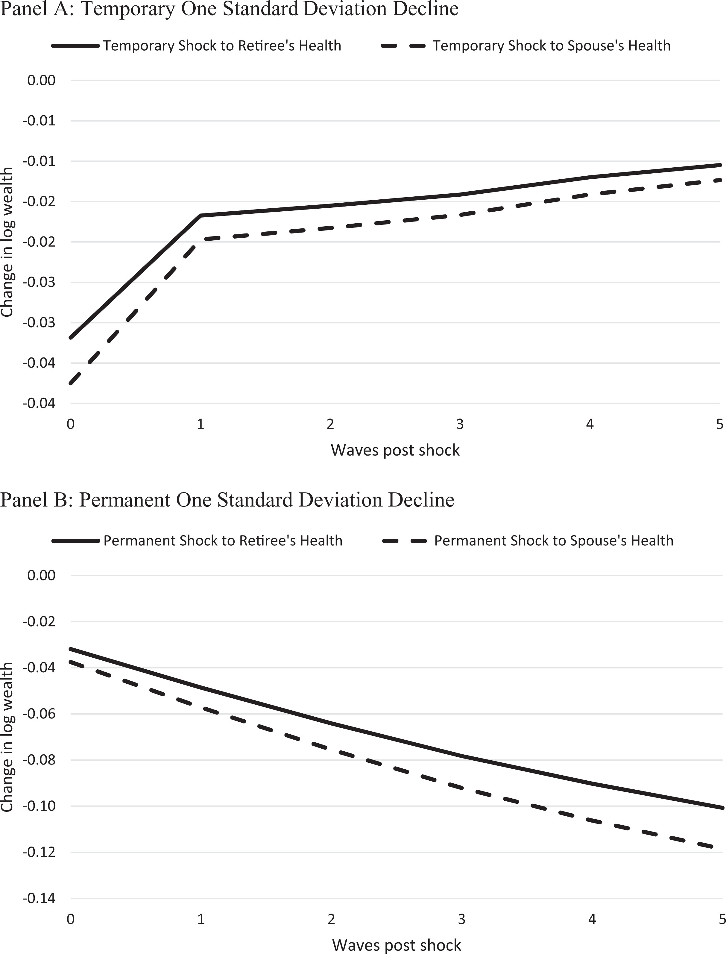
The estimated effect of a (one wave) standard deviation decrease in health score on log wealth (simulations based on estimates from Table 2, column 3).

Panel B of Figure 5 uses our preferred estimates to simulate the wealth response to a permanent one SD decrease in male retiree and spousal health scores. Permanent shocks tend to be the norm for this population. As with the transitory (one wave) shocks, the initial effect of a permanent decrease in health scores is given by the coefficient on the health score variables. However, while the response to a transitory shock is characterized by an adjustment back to the original steady state, the response to a permanent shock is characterized by an adjustment to a new (lower) steady-state level of household wealth. Moreover, the new steady-state postshock level of wealth is determined by the long-run multipliers, 5.4 in the case of our preferred specification, multiplied by the initial effect of the health shock. Thus, using our preferred specification, the long-run impact of a permanent one SD decline in retiree and spousal health is to decrease wealth by 17% and 20%. Over 50% of the adjustment to these new steady-state values of household wealth is complete within the first-five waves (10 years) following a shock. Given life expectancies for retirees, particularly those who experience large negative health shocks, and the slow adjustment to steady state implied by the models, it is extremely unlikely that retirees would live long enough to experience the full adjustment to steady state following a permanent health shock.

Conclusion

This article uses data on a sample of retirees from the HRS to pursue to (1) describe the changes in health status that occur in the retirement years, (2) to examine the extent to which the declines in health that are common in retirement lead to the erosion of wealth. Understanding of these issues has implications for both the point-in-time assessment of the sufficiency of adequacy of wealth holding in retirement and the design of private and public pension and health insurance programs.

In order to assess changes in health following retirement, a broad measure of physical health using the framework of IRT is constructed. This health measure, which makes use of 21 of health indicators available in the HRS in Waves 2 through 10, offers several advantages relative to approaches to measuring health. This IRT-based measure is able to measure health when a subset of the items used to construct the measure are missing and has the ability to reliably measure health across the spectrum of retiree health. We find that average health declines over retirement years, but that these declines are larger for individuals who are in better health at the time of retirement. Retirees face substantial risk of negative shocks to their and their spouses health with shocks of one SD (either from baseline or on a wave-to-wave basis) occurring for an estimated one third of the population by the 10th-year postretirement. We also find that large declines in health are more permanent than transitory in that recovery from large health shocks is uncommon with further deterioration of health and death far more likely outcomes.

When large declines in health do occur, they have a sizable and measurable effect on wealth. Using dynamic panel data models which allow for the assessment of both short- and long-run effects of changes in health status on wealth, we find that temporary (one wave) SD decrease in health will lead to an immediate loss of wealth in the neighborhood of 3–6%, and the smaller effects thereafter as the results of the shock slowly dissipate. Large permanent declines in health will lead to similar percentage declines initially but grow larger as wealth adjust to a new, lower, steady-state level. By the 10th year after the shock, the effect of an SD decline in retiree or spousal health is estimated to be in the range of 10–12% with the larger effects attributed to a decline in spousal health.²⁶

This finding of large long-run effects of permanent health declines on wealth has implications for both the optimal behavior of individuals entering retirement and for the design of public pension and health insurance programs. In particular, our findings raise the question of whether retirees should self-insure to a greater extent than currently do, perhaps through the purchase of Medigap plans and long-term care insurance, and/or whether society should provide more insurance on their behalf, perhaps through the public provision of long-term care insurance or lower rates of Medicare cost sharing.

Footnotes

Appendix

Table A1.

Items Utilized in the Construction of IRT-Based Health Measures.

Item Number	Item Description
1	No reported difficulty dressing (=1)
2	No reported difficulty bathing/showering (=1)
3	No reported difficulty eating (=1)
4	No reported difficulty getting out of bed (=1)
5	No reported difficulty walking across the room (=1)
6	No reported difficulty walking one block (=1)
7	No reported difficulty walking several blocks (=1)
8	No reported difficulty jogging one mile (=1)
9	No reported difficulty sitting (=1)
10	No reported difficulty getting out of a chair (=1)
11	No reported difficulty climbing a flight of stairs (=1)
12	No reported difficulty climbing several flights of stairs (=1)
13	No reported difficulty stooping/bending over (=1)
14	No reported difficulty picking up a heavy object (=1)
15	No reported difficulty picking up a dime (=1)
16	No reported difficulty reaching above head (=1)
17	No reported difficulty pushing or pulling a heavy object (=1)
18	Has been in the hospital since last wave (=1)
19	Has been in a nursing home since last wave (=1)
20	Has had home care since last wave (=1)
21	Self-reported health (0 = poor, 4 = excellent)

Note. In some instances, respondents report that they do not engage in a particular activity, without indicating whether or not they have difficulty with said activity. In these instances, we assume an item value of zero. IRT = item response theory.

Declaration of Conflicting Interests

The author(s) declared no potential conflicts of interest with respect to the research, authorship, and/or publication of this article.

Funding

The author(s) received no financial support for the research, authorship, and/or publication of this article.

Notes

References

Arellano

Bond

(1991). Some test of specification for panel data: Monte Carlo evidence and application to employment equations. Review of Economic Studies, 58, 277–297.

Arellano

Bover

(1995). Another look at instrumental variables estimation of error-component models. Journal of Econometrics, 68, 29–51.

Baker

(2001). The basics of item response theory. ERIC Clearinghouse on Assessment and Evaluation, University of Maryland, College Park, MD.

Bernheim

B. D.

(1992). Is the baby boom generation preparing adequately for retirement? (Technical Report, Unpublished). New York, NY: Merrill Lynch and Company.

Blundell

Bond

(1998). Initial conditions and moment conditions in dynamic panel data models. Journal of Econometrics, 87, 115–143.

Bowsher

C. G.

(2002). On testing overidentifying restrictions in dynamic panel data models. Economics Letters, 77, 211–220.

Butrica

B. A.

Iams

H. M.

Smith

K. E.

(2003). The changing impact of social security on retirement income in the United States. Social Security Bulletin, 65, 1–13.

Butrica

B. A.

Iams

H. M.

Smith

K. E.

(2007). Understanding baby boomer retirement prospects. In Bridget

Mitchell

O. S.

Soldo

B. J.

(Eds.), Redefining retirement: How will boomers fare? (pp. 70–94). Oxford, England: Oxford University Press.

Coile

Milligan

(2009). How household portfolios evolve after retirement: The effect of aging and health shocks. Review of Income and Wealth, 55, 226–248.

10.

Committee to Evaluate Measures of Health Benefits for Environmental, Health, and Safety Regulation, Board on Health Care Services, Institute of Medicine. (2006). Valuing health for regulatory cost-effectiveness analysis. Washington, DC: National Academies Press.

11.

Engen

E. M.

Gale

W. G.

Uccello

C. E

. (1999). The adequacy of household saving. Brookings Papers on Economic Activity, 2, 65–187.

12.

Fryback

D. G.

Palta

Cherepanov

Bolt

Kim

J.-S.

(2010). Comparison of 5 health-related quality-of-life indexes using item response analysis. Medical Decision Making, 30, 5–15.

13.

Gustman

A. L.

Steinmeier

T. L.

(1998). Effects of pensions on saving: Analysis with data from the health and retirement study (NBER Working Paper No. 6681). Cambridge, MA: National Bureau of Economic Research.

14.

Haveman

Holden

Romanov

Wolfe

(2007a). Assessing the maintenance of savings sufficiency over the first decade of retirement. International Tax and Public Finance, 14, 481–502.

15.

Haveman

Holden

Romanov

Wolfe

(2007b). The sufficiency of retirement savings: A comparison of two cohorts of retired workers at the time of retirement. In Bridget

Mitchell

O. S.

Soldo

B. J.

(Eds.), Redefining retirement: How will boomers fare? (pp. 36–69). Oxford, England: Oxford University Press.

16.

Haveman

Holden

Wolfe

Sherlund

(2006). Do newly retired workers in the United States have sufficient resources to maintain well-being? Economic Inquiry, 44, 249–264.

17.

Hayes

R. D.

Morales

L. S.

Reise

S. P.

(2000). Item response theory and health outcomes measurement in the 21st century. Medical Care, 8, 28–42.

18.

Holden

Schrass

. (2015). The role of IRAs in U.S. households’ saving for retirement. ICI Research Perspective, 21. Retrieved from https://www.ici.org/pdf/per22-01.pdf

19.

Lindebloom

van Doorslaer

(2004). Cut point shift and index shift in self-reported health. Journal of Health Economics, 23, 1083–1099.

20.

Megbolugbe

Sa-Aadu

Shilling

(1997). Oh yes, the elderly will reduce housing equity under the right circumstances. Journal of Housing Research, 8, 53–74.

21.

Megbolugbe

Sa-Aadu

Shilling

(1999). Elderly female-headed households and the decision to trade down. Journal of Housing Economics, 8, 285–300.

22.

Miller

Robinson

L. A.

Lawrence

R. S.

(Eds.). (2006). Valuing health for regulatory cost-effectiveness analysis. Washington, DC: Committee to Evaluate Measures of Health Benefits for Environmental, Health, and Safety Regulation, Institute of Medicine. Retrieved from http://www.nap.edu/catalog/11534.html

23.

Mitchell

O. S.

Moore

Phillips

(2000). Explaining retirement saving shortfalls. In Mitchell

O. S.

Hammond

P. B.

Rappaport

(Eds.), Forecasting retirement needs and retirement wealth (pp. 139–166). Philadelphia, PA: University of Pennsylvania Press.

24.

Moore

Mitchell

O. S.

(2000). Projected retirement wealth and saving adequacy. In Mitchell

O. S.

Hammond

P. B.

Rappaport

A. M.

(Eds.), Forecasting retirement needs and retirement wealth (pp. 68–94). Philadelphia, PA: University of Pennsylvania Press.

25.

Nickell

S. J.

(1981). Biases in dynamic models with fixed effects. Econometrica, 49, 1417–1426.

26.

Poterba

Venti

S. F.

Wise

D. A.

(2011). Family status transitions, latent health, and the post-retirement evolution of assets. In Wise

D. A.

(Ed.), Explorations in the economics of aging (pp. 23–74). Chicago, IL: University of Chicago Press.

27.

Roodman

(2009). How to do xtabond2: An introduction to ‘difference’ and ‘system’ GMM in Stata. Stata Journal, 9, 86–136.

28.

Scholz

J. K.

Sheshadri

Khitatrakun

(2006). Are Americans saving optimally for retirement? Journal of Political Economy, 114, 607–643.

29.

Smith

J. P.

(1999). Healthy bodies and thick wallets: The dual relation between health and economic status. Journal of Economic Perspectives, 13, 145–166.

30.

Venti

S. F.

Wise

D. A.

(2002). Aging and housing equity. In Mitchell

O. S.

Bodie

Hammond

P. B.

Zeldes

(Eds.), Innovations in retirement financing (pp. 254–281). Philadelphia, PA: University of Pennsylvania Press.

31.

Venti

S. F.

Wise

D. A.

(2004). Aging and housing equity: Another look. In Wise

D. A.

(Ed.), Perspectives in the economic of aging (pp. 127–180). Chicago, IL: University of Chicago Press.

32.

Wallace

G. L.

Haveman

Holden

Wolfe

(2010). Trigger Events and Financial Outcomes Among Older Households. Center for Financial Security Working Paper WP 10-2, University of Wisconsin, Madison. Retrieved from https://centerforfinancialsecurity.files.wordpress.com/2010/09/2010-trigger-events-and-financial-outcomes-paper.pdf

33.

Wallace

G. L.

Haveman

Holden

Wolfe

(2013). Health and wealth in early retirement. In Couch

Daly

Zissimopoulos

(Eds.), Life cycle events and their consequences: Job loss, family change, and declines in health. Stanford, CA: Stanford University Press.

34.

Wolff

E. N.

(2002). Retirement insecurity: The income shortfalls awaiting the soon-to-retire. Washington, DC: Economic Policy Institute.