
Abstract
Directional dependency is a method to determine the likely causal direction of effect between two variables. This article aims to critique and improve upon the use of directional dependency as a technique to infer causal associations. We comment on several issues raised by von Eye and DeShon (2012), including: encouraging the use of the signs of skewness and excessive kurtosis of both variables, discouraging the use of D’Agostino’s K 2, and encouraging the use of directional dependency to compare variables only within time points. We offer improved steps for determining directional dependency that fix the problems we note. Next, we discuss how to integrate directional dependency into longitudinal data analysis with two variables. We also examine the accuracy of directional dependency evaluations when several regression assumptions are violated. Directional dependency can suggest the direction of a relation if: (a) the regression error in population is normal; (b) an unobserved explanatory variable correlates with any variables equal to or less than .2; (c) a curvilinear relation between both variables is not strong (standardized regression coefficient ≤ .2); (d) there are no bivariate outliers; and (e) both variables are continuous.
Directional dependency is a method to determine the likely causal direction of effect between two variables (Dodge & Rousson, 2000). Directional dependency can help to determine which of two correlation variables can be designated as the explanatory variable. It is determined by comparing the shapes of the distributions of two continuous random variables. This article aims to provide a brief overview of directional dependency, critique and improve upon the use of the directional dependency tests presented by von Eye and DeShon (2012), and address the circumstances in which tests of directional dependency are appropriate.
This article is divided into several parts. First, we define skewness, kurtosis, and excessive kurtosis. We then show that skewness and excessive kurtosis (which is sometimes confused with kurtosis) can be used to examine directional dependency (Dodge & Rousson, 2000, 2001; Dodge & Yadegari, 2010). Third, we comment on several issues raised by von Eye and DeShon (2012), including: encouraging the use of the signs of skewness and excessive kurtosis of both variables; discouraging the use of D’Agostino’s K 2; and showing that the test of directional dependency is only appropriate with concurrent data and cannot be used to determine the direction of effects over time. We then offer improved steps for determining directional dependency that fix the problems we note. In this regard, we discuss how to integrate directional dependency into longitudinal data analysis with two variables. Finally, we clarify the (in)accuracy of directional dependency tests when assumptions of regression analysis are violated.
Definitions
We begin with definitions that are needed below. Skewness (
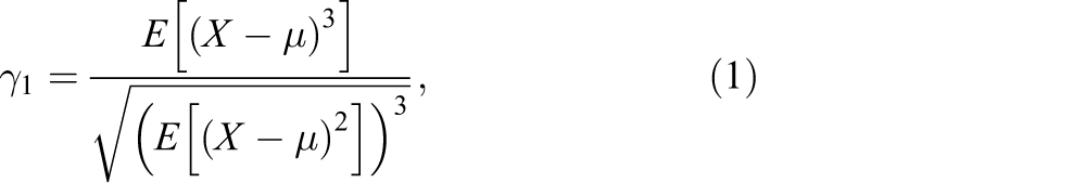
where X is the target random variable, E is the expectation function or the average of the argument,
Kurtosis (
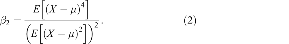
All notations are defined in equation 1 (see online Appendix A for definitions, derivations, and proofs; also at crmda.ku.edu/supplementals). The kurtosis of a normal distribution is 3.
Excessive kurtosis (

Therefore, the excessive kurtosis of a normal distribution is 0. Some articles use the term “kurtosis” when they mean “excessive kurtosis.” Differentiating between kurtosis and excessive kurtosis is essential to understand directional dependency and its calculation. Equations 1 and 3 are population-level estimates of skewness and excessive kurtosis.
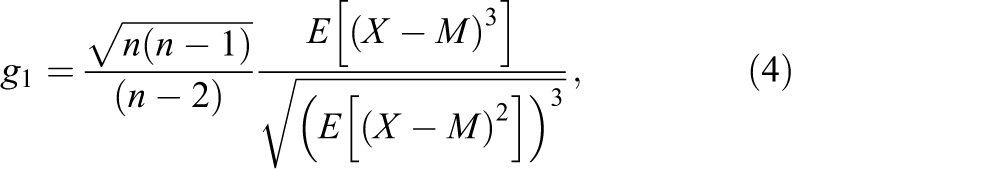
The unbiased sample estimator of skewness and excessive kurtosis takes a different functional form from their population formulas. The sample estimates of skewness (
and
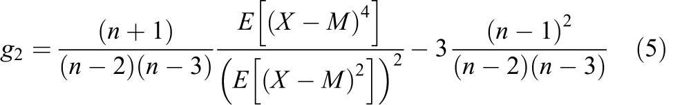
where M is the sample mean, E is the expectation (average) function, and n is the sample size.
Directional dependency principle
Although a large part of this section is redundant to the proof from Dodge and Rousson (2000, 2001), Muddapur (2003), and Dodge and Yadegari (2010), we repeat this proof for the sake of clarity and because this proof is needed for additional proof in the following sections.
Dodge and Rousson (2000, 2001) showed that directional dependency can be determined by the proportion of skewness of two variables, X and Y. They compared two models:

and

where


The possible explanations of causal inference within a two-variable relation.
and the fourth power of the correlation between both variables (Dodge & Yadegari, 2010) is equal to the ratio of the excessive kurtosis of Y (

Equations 8 and 9 will only hold if the regression error (e) is normally distributed.
Dodge and Rousson (2000, 2001) proposed that directional dependency can be determined based on the possible range of the cube of a correlation coefficient. Because the cube of a correlation will range between −1 and 1 (i.e.,

where |…| is the absolute value function. In other words, if X is the predictor and Y is the outcome, then the absolute value of the skewness of Y would be less than the absolute value of the skewness of X. Because the fourth power of a correlation coefficient ranges from 0 to 1 then, based on equation 9, the magnitude of the excessive kurtosis of Y will not be greater than the magnitude of the excessive kurtosis of X (Dodge & Yadegari, 2010):

Comments on von Eye and DeShon (2012)
The proof shown in the previous section leads to seven general comments on von Eye and DeShon (2012). Some comments are applicable to the methods proposed by Dodge and Rousson (2000, 2001) and Dodge and Yadegari (2010) as well.
Using excessive kurtosis instead of kurtosis
Von Eye and DeShon’s (2012) paper is not clear on how they define kurtosis. They use
The summary of using the skewness or excessive kurtosis for determining directional dependency between two variables at the population and sample levels

The simulation results of directional dependency if a covariate exists and the correlation between explanatory and response variables are .2 (
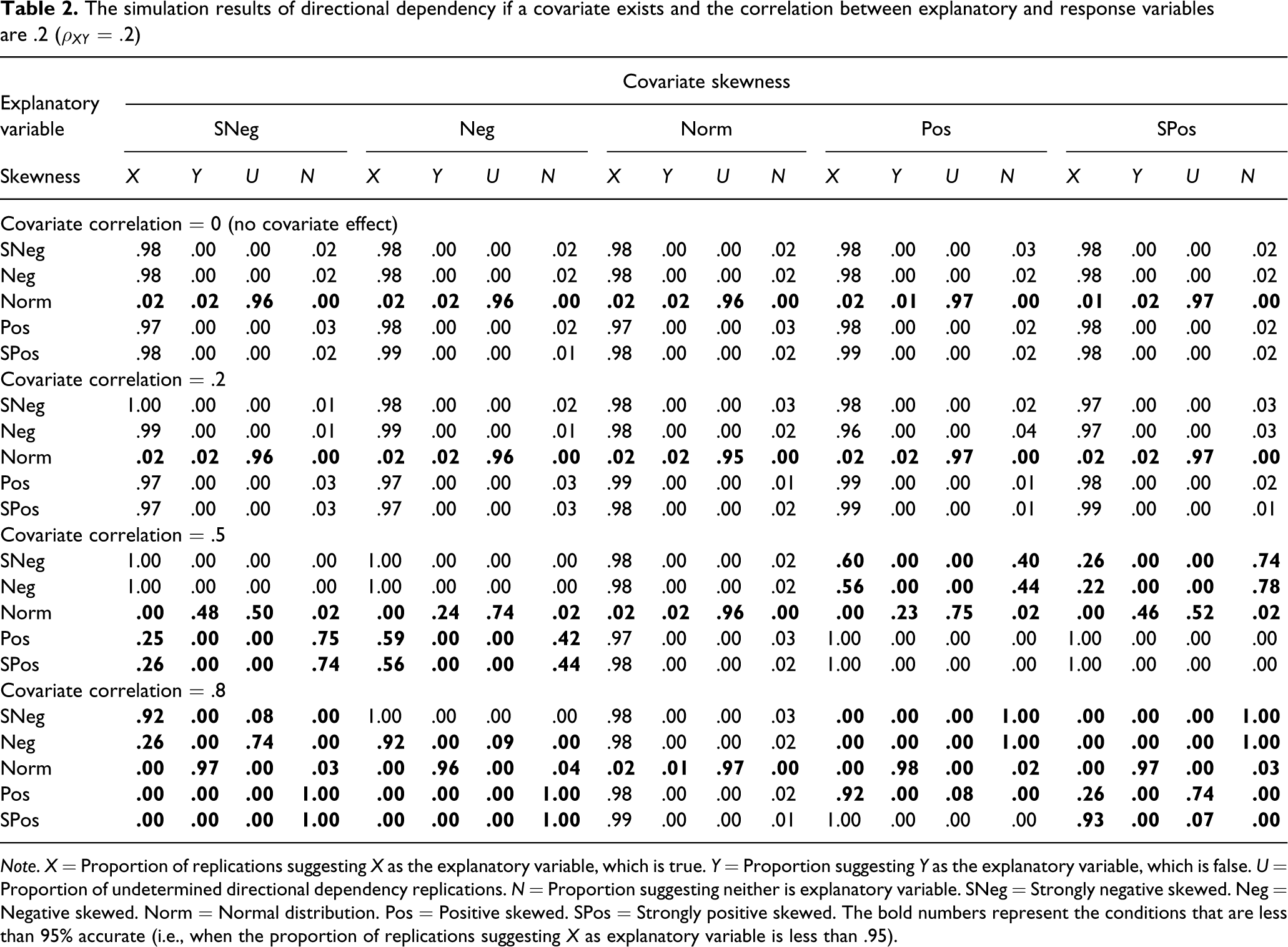
Note. X = Proportion of replications suggesting X as the explanatory variable, which is true. Y = Proportion suggesting Y as the explanatory variable, which is false. U = Proportion of undetermined directional dependency replications. N = Proportion suggesting neither is explanatory variable. SNeg = Strongly negative skewed. Neg = Negative skewed. Norm = Normal distribution. Pos = Positive skewed. SPos = Strongly positive skewed. The bold numbers represent the conditions that are less than 95% accurate (i.e., when the proportion of replications suggesting X as explanatory variable is less than .95).
The simulation results of directional dependency if a covariate exists and the correlation between explanatory and response variables are .5 (
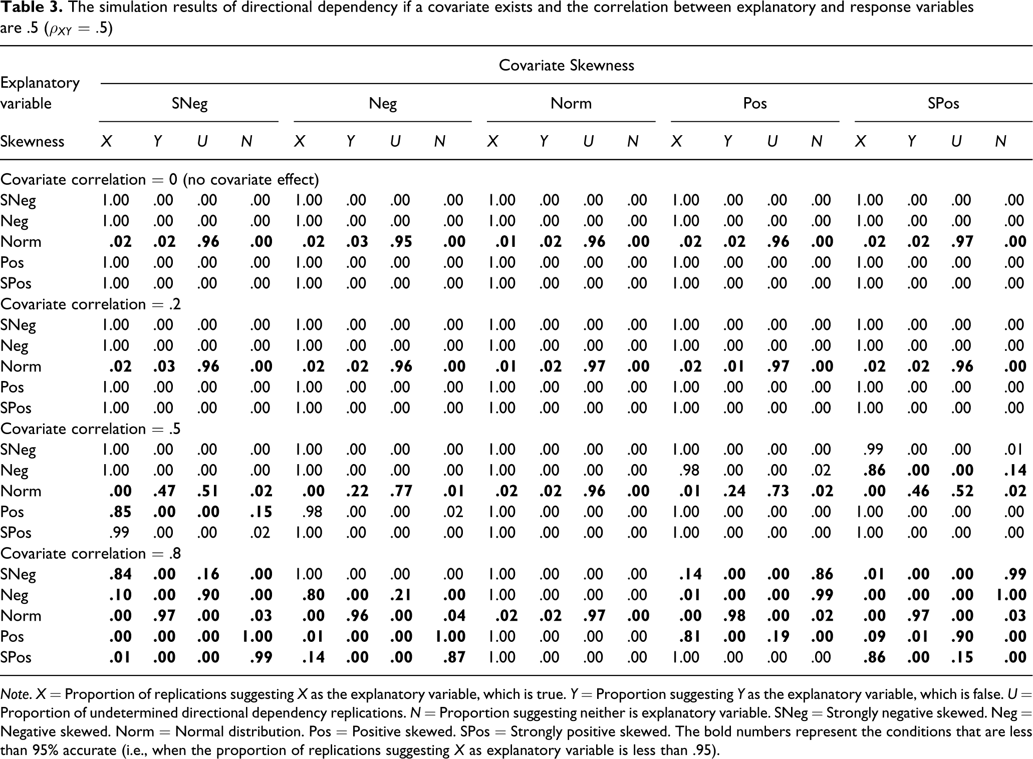
Note. X = Proportion of replications suggesting X as the explanatory variable, which is true. Y = Proportion suggesting Y as the explanatory variable, which is false. U = Proportion of undetermined directional dependency replications. N = Proportion suggesting neither is explanatory variable. SNeg = Strongly negative skewed. Neg = Negative skewed. Norm = Normal distribution. Pos = Positive skewed. SPos = Strongly positive skewed. The bold numbers represent the conditions that are less than 95% accurate (i.e., when the proportion of replications suggesting X as explanatory variable is less than .95).
Accounting for the sampling error of the difference
Von Eye and DeShon (2012) acknowledged the sampling error of skewness and excessive kurtosis by proposing that the skewness (or excessive kurtosis) of at least one variable should be significant before determining directional dependency. The sampling error of the difference in skewness (or excessive kurtosis), however, was not accounted for. Because of the sampling error, the difference in skewness in the population is always different from the difference in skewness in the sample to some extent, especially when sample size is small. In some situations, the differences in skewness in population and in sample have different signs. For example, the skewness of X can be greater than the skewness of Y in the sample, when in fact the skewness of X is less than the skewness of Y in the population. To determine directional dependency, the difference in magnitude of skewness and excessive kurtosis must be significant. The significance of the difference in skewness (or excessive kurtosis) guarantees that the differences in population and sample levels have the same sign. Otherwise, the skewness (or excessive kurtosis) of X may be either greater or less than the skewness (or excessive kurtosis) of Y in the population and the decision is inconclusive.
Accounting for other possible two-variable associations
Directional dependency is designed to choose whether the effect is from X to Y (Figure 1a) or from Y to X (Figure 1b). Von Eye and DeShon (2012) do not discuss the possibility of a non-recursive effect (Figure 1c) or an unobserved explanatory variable (Figure 1d). A non-recursive effect is when X and Y affect each other simultaneously. An unobserved explanatory variable means an extraneous variable, Z, affects both X and Y but X and Y have no causal effect between each other, which would be a spurious effect. The directional dependency technique assumes one direction of effect between two variables with no extraneous variables.
Accounting for the signs of skewness and excessive kurtosis
Dodge and Rousson (2000, 2001), Dodge and Yadegari (2010), and von Eye and DeShon (2012) focused only on comparing the magnitudes of skewness and excessive kurtosis to determine directional dependency. The signs of skewness and excessive kurtosis are critical as well.
From equation 8, the correlation coefficient as well as the cube of the correlation coefficient is positive if, and only if, the skewness of X and Y have the same sign. The correlation coefficient, as well as the cube of the correlation coefficient, is negative if, and only if, the skewness of X and Y have different signs. If the skewness signs are inconsistent with the sign of the correlation coefficient (e.g., the correlation is positive whereas the signs of skewness of both variables are different), equation 8 is not satisfied. Thus neither X (equation 6) nor Y (equation 7) is an explanatory variable (the relation may be non-recursive or spurious). The excessive kurtosis of X and Y must have the same sign because
Ignoring the signs of skewness and excessive kurtosis can lead to a different conclusion. We illustrate this issue in von Eye and DeShon’s (2012) example of the relation between attention deficit hyperactivity disorder (ADHD) symptoms and the blood lead level. The skewness of blood lead level and inattentive symptoms are 2.156 and −0.815, respectively. With a standard error of 0.198, the blood lead level variable is positively skewed and the inattentive symptom variable is negatively skewed in the population. If von Eye and DeShon’s (2012) guideline is used, blood lead level is suggested as the explanatory variable. Presumably, the correlation between ADHD symptoms and the blood lead level is positive. To support directional dependency, however, these variables must have the same signs. Because they have different signs, neither variable is supported as the explanatory variable.
We assume that the kurtosis reported in von Eye and DeShon (2012) is excessive kurtosis (
Avoiding the use of D’Agostino’s K 2
Our next point is on the use of D’Agostino’s K 2 (1971) statistic for directional dependency. Even though the use of this index for testing directional dependency was supported by von Eye and DeShon’s (2008) simulation, the use of K 2 can be misleading because the directional dependency of both skewness and excessive kurtosis must each be supported individually. If the directional dependency of skewness indicates that one variable is an explanatory variable, the directional dependency of excessive kurtosis should also indicate that the variable is an explanatory variable or at least that the directional dependency status is undetermined. The directional dependency of excessive kurtosis should not contradict the directional dependency indicated by using skewness.
By combining both skewness and excessive kurtosis into a single index, the information of individual directional dependency indices is lost. For example, in the directional dependency of lead level and hyperactive-impulsive symptoms in von Eye and Deshon (2012), the skewness shows that lead level (
The need to establish the two-variable relation
Another important issue in determining directional dependency is that the relation between two variables must be established. Von Eye and DeShon (2012) emphasized comparing the degree of non-normality between both variables; however, the establishing of a non-zero relation between two variables needs to be explicitly mentioned as well. One of the central conditions of causal inference is that a non-zero relation must exist between the variables (Cook & Campbell, 1979). We mention this issue because we are afraid that one may pick a pair of unrelated and non-normal variables (i.e., neither equation 6 or 7 is true in the population) and then compare skewness or excessive kurtosis directly to infer the direction of an effect. This practice will produce type I errors—inferring a direction of effect when there is no effect. Therefore a relation between both variables must exist before examining directional dependency.
Avoiding the use of directional dependency in longitudinal data
Von Eye and DeShon (2012) proposed two scenarios that applied directional dependency within a longitudinal data analysis context, each with multiple time points. In scenario 1, X is observed at time 2 only and Y is observed at both time 1 and time 2. They proposed that, if X is the explanatory variable that is active on time 2 only, then (a) Y should have less skewness at time 2 than at time 1, and (b) X should have more skewness than Y at time 2. In scenario 2, X is observed in time 1 only and Y is observed at both time 1 and time 2. They proposed that if X is the explanatory variable that is active at time 1 only, then (a) Y should have more skewness at time 2 than at time 1, and (b) X should have more skewness than Y at time 1.
We disagree with the first rule in determining directional dependency from both scenarios. The rule implies that the response variable measured when an explanatory variable is active will be closer to a normal distribution than one measured when the explanatory variable is not active. This argument is not necessarily true. Consider three propositions here: From the directional dependency principle (i.e., equations 8 and 9), a response variable is not normally distributed when the response variable has a predictor that is not normally distributed. Many psychological variables deviate significantly from a normal distribution (Micceri, 1989). As one of the assumptions of science, every effect (variable) has its cause (Maxwell & Delaney, 2004).
From proposition 3, a variable exists because it has a cause. From proposition 1, a psychological variable is not normally distributed if its cause is not normally distributed. Thus a psychological variable must have an unobserved explanatory variable that makes them not normally distributed. In terms of mathematical notation, let Y be the psychological variable and Z be its unobserved cause. The regression model is:
where 
and
where Y
1 and Y
2 are the response variable at time 1 and time 2, respectively, Z
1 and Z
2 are the response variable’s unobserved cause at time 1 and time 2, respectively,
Assuming that X and Z are independent and e
1 and e
2 are normally distributed, as shown in online Appendix A (also at crmda.ku.edu/supplementals), the ratio of the skewness of Y when X is active to the skewness of Y when X is inactive is
where
The key implication of equation 15 is that the skewness of X can make the ratio of the skewness of Y 1 and Y 2 either greater or less than 1. This possibility means that the skewness of Y at time 1 (X is active) is not necessarily greater than the skewness of Y at time 2 (X is inactive). Therefore the skewness of the response variable should not be compared across time to determine directional dependency.
Improved rules for determining directional dependency
On the basis of the above, we offer improved rules for determining directional dependency. At the population level, the upper part of Table 1 shows a summary of using skewness and excessive kurtosis for directional dependency tests. The rules at the population and sample levels are different because of sampling error. The decision steps are:
If the correlation between X and Y is significant, go to the next step. If not, neither variable is the explanatory variable. If If the correlation is positive and both If If If the correlation between X and Y is significant, go to the next step. If not, neither variable is the explanatory variable. If If both If If
The decision steps for comparing excessive kurtosis at the sample level are:
The lower part of Table 1 shows a summary of using skewness and excessive kurtosis for directional dependency tests at the sample level after a significant correlation between both variables is determined. All significance tests are easily done by using a simple bootstrap estimation method (Efron & Tibshirani, 1993). We provide an R script in online Appendix B (also at crmda.ku.edu/supplementals) to run a bootstrap confidence interval for correlation, skewness, excessive kurtosis, and the difference in magnitudes of skewness and excessive kurtosis.
One prospective problem of a step approach is the inflation of type I error. Because a step approach involves multiple significance testing, the chance that at least one test is a type I error is greater than the specified alpha level for an individual test. The meaning of type I error in this situation, however, is different from the multiple comparisons in the analysis of variance. Overall type I error in this situation, in our opinion, is the probability that the directional dependency test suggests that X, Y, or neither is the explanatory variable when a decision of undetermined directional dependency should be selected based on the information at the population level. We will discuss this issue in the following section after we show our Monte Carlo simulation results.
Guidelines of using directional dependency in longitudinal data
As explained earlier, the proposed method for directional dependency determination is invalid in comparing between the same (or different) variables across time points. If longitudinal data can be obtained, causal inference is conducted more rigorously than in a cross-sectional analysis because temporal precedence can be supported (i.e., a cause precedes an effect; Cook & Campbell, 1979). Figure 2 show the list of possible two-variable relationships in a longitudinal design: (a) X is explanatory; (b) Y is explanatory; (c) X and Y have no relationship; (d) X and Y have reciprocal relationship; and (e) X and Y have spurious relationship. We assume that the causal structure does not change across time (i.e., stationary; Kenny, 1979). If X and Y are observed, we can test models a, b, c, and d directly by nested model comparison using structural equation modeling (chi-square difference test). If the observed data comes from model E and only X and Y are observed, model D would be selected by the nested model comparison.

The possible explanations of causal inference within a two-variable relation in a longitudinal design.
The proposed directional-dependency method cannot replace the nested model comparison. This method can be used as additional information in causal inference by comparing different variables at the same time point. When model a is selected by the nested model comparison, the directional dependency should suggest that X is explanatory or the directional dependency is undetermined at time point 2 and again at time point 3. When model b is selected, the directional dependency should suggest that Y is explanatory or the directional dependency is undetermined. When model c or d is selected (model c, d, and e might be true in the population), the directional dependency should suggest that neither variable is explanatory or the directional dependency is undetermined. Thus directional dependency tests can be used as an additional method for causal inference in a longitudinal design, but directional dependency cannot be applied over time.
Robustness of assumption violations
Directional dependency is based on regression analysis which has several assumptions. Therefore the (in)accuracy of directional dependency will be related to the violation of the regression assumptions to some degree. We highlight some important assumptions of basic regression analysis that would decrease the accuracy of any test of directional dependency. Those assumptions are: (a) normality; (b) no unobserved explanatory variable exists; (c) the relation between X and Y is linear; (d) no outlier; and (e) the response variable is continuous.
Normality
Regression analysis and directional dependency assume that the error is normally distributed at the population level. If this assumption is not true, equations 8–11 will not hold. The sample distribution, instead of the population distribution, is usually observed. Because of sampling error, the sample residual distribution need not be exactly normal, although it should be close to normal if it comes from a normal population error. When X or Y is suggested as the explanatory variable, the suggested (explanatory) variable and the other (response) variable can be used to find the sample regression residual. For example, if X is suggested as the explanatory variable, Y is regressed on X and the residual is saved. The residual is checked for normality (Maxwell & Delaney, 2004).
Unobserved explanatory variable
Directional dependency only focuses on the effect of one independent variable on one dependent variable. A dependent variable, however, may be caused by more than one variable. Unobserved explanatory variables (i.e., other predictor variables) might lead to erroneous conclusions in directional dependency. For example, X and Z are explanatory variables; X is normally distributed and observed while Z is highly skewed but unobserved. In this situation, Y (the dependent variable) will be skewed because of the skewness of Z. If directional dependency between X and Y is of interest, a researcher would errantly pick Y as the explanatory variable.
We will further investigate the effect of an unobserved explanatory variable by a mathematical proof and a Monte Carlo simulation. The mathematical proof (as shown in online Appendix A, also at crmda.ku.edu/supplementals) illustrates how an unobserved covariate affects directional dependency tests. The following Monte Carlo simulation examines the robustness of directional dependency on an unobserved explanatory variable. This simulation study result shows the robustness to violations of other regression assumptions described below as well.
In this simulation, X is an explanatory variable, Y is a response variable, and Z is a covariate. X and Z were independent ( Skewness of explanatory variable: strongly negative ( Skewness of covariate: strongly negative, negative, normal, positive, and strongly positive. Correlation (standardized regression coefficient) between the response variable and the explanatory variable: .2 and .5. Correlation (standardized regression coefficient) between the response variable and the covariate: 0 (baseline model), .2, .5, and .8.
To create different levels of skewness, we used a χ
2 distribution. The χ
2 distribution has a higher level of skewness if its degree of freedom is low. In the strongly negative and the strongly positive skewness condition we used the χ
2 distribution with two degrees of freedom. In the negative and the positive skewness condition we used the χ
2 distribution with 10 degrees of freedom. In the normal condition we used a standard normal distribution. We used a sample size of 1,000 and ran 1,000 replications per condition. We used X as the explanatory variable and our proposed method of detection (online Appendix B contains the R script used; also at crmda.ku.edu/supplementals). We used skewness (g
1) to determine directional dependency only. A simulation using von Eye and DeShon’s (2012) method is available in online Appendix C.
The simulation study show the results when the correlations between X and Y are .2 and .5, respectively (Tables 2 and 3). The rows of both tables are divided into four panels that represent the correlation between Y and Z (0, .2, .5, and .8, respectively). There are four possible results from the directional dependency test: X is the explanatory variable, Y is the explanatory variable, neither is the explanatory variable, or the directional dependency is undetermined. Each cell represents the proportion that the directional dependency showed each possible result.
The first panel of rows of both tables is the baseline model without the covariate effect. When the explanatory variable is skewed, the directional dependency can be determined almost 100% correctly. On the other hand, if the explanatory variable is normal, approximately 96% of replications were undetermined, 2% of replications suggested X as an explanatory variable, and 2% of replications suggested Y as an explanatory variable. The similar pattern of result is generalized to the second panel of rows of both tables when the effect of the covariate is small (i.e., the correlation between covariate and response variable is .2).
The third and fourth panels of rows of both tables represent the conditions where the effect of the covariate is medium (
From this simple simulation we can conclude that the test of directional dependency is robust to the small effect of an unobserved explanatory variable. When the covariate effect is medium or large, the result cannot be trusted because the skewness of a variable can result from either itself or the covariate. Thus directional dependency can only be trusted if the existence of a non-trivial, unobserved explanatory variable can be ruled out. In other words, the correlations of the covariate with both variables used in directional dependency should not exceed .2.
From this simulation, type I error can be examined when X is normal and the correlation between X and Z is 0 (the third row of the first panel). In this situation, the decision should be that the directional dependency is undetermined (see the top panel of Table 1). The proportion that the test suggested “undetermined” is .96. That is, the overall type I error is .04, which is close to the nominal level of .05 even though this step approach involves multiple testing.
Another issue related to unobserved explanatory variables is that the correlation between two variables may be spurious (Figure 1d). Thus the potential for a spurious correlation must also be ruled out before investigating the directional dependency. Here, if there is no potential effect of a covariate that is greater than a standardized regression coefficient on either variable of .2, the spurious contribution to a correlation will not be greater than .04. This magnitude of correlation is sufficiently trivial to ignore in a test of directional dependency. The existence of a nontrivial unobserved variable is similar to the elimination of plausible alternative causes in causal relation inference (Cook & Campbell, 1979). Instead of totally eliminating alternative causes, however, the alternative causes should have effects that are not too strong to compromise the accuracy of directional dependency. Conducting tests of plausible third variables would be a recommended step to ensure that the directional dependency tests are accurate.
Curvilinear relation
Dodge and Rousson (2001) indicated that the test of directional dependency is applicable for a linear relation. No effect between two variables, however, is exactly linear in the population (MacCallum & Austin, 2000). There will be curvatures in a relation to some degree. Consider the quadratic effect of a predictor. In multiple regression, a quadratic effect can be modeled as:
where
Outliers
Outliers can be considered as unobserved explanatory variables. If one observation is an outlier, the outlier can be modeled by a dummy variable (1 = outlier and 0 = others), D, as
where
The mathematical proof (as shown in online Appendix A, also at crmda.ku.edu/supplementals) and the simulation study in the unobserved explanatory variable section also apply. Specifically, the effect size of the outlier (standardized regression coefficient) is the most important factor. If the correlation between a dummy variable indicating the outlier (D) and the dependent variable (Y) is 0, the effect size of the outlier is also 0 and the directional dependency will not be biased. That is, if the averages of the dependent variable between the outlier and other observations are not different, directional dependency determination is not biased. Therefore the outlier influence is negligible when the outlier is univariate or in X only. If an outlier is bivariate, the outlier should be excluded (Cohen, Cohen, West, & Aiken, 2003).
Beyond the general linear model
The test for directional dependency is based on the general linear model assuming that the response variable is continuous and the relation is linear. The general linear model is not an exhaustive list of all two-variable relations. In fact, the general linear model is a submodel of the generalized linear model with a link function that is 1.0 (identity link). Directional dependency is not applicable for other submodels in the generalized linear model. For example, Poisson regression is usually used to predict count variables (such as hours of exercise), which is the submodel of the generalized linear model with log link function and a Poisson distribution. In this submodel, a dependent variable may have a higher magnitude of skewness than an explanatory variable (i.e., a Poisson distribution is positively skewed when the rate is low).
In the example of the relation between ADHD and the number of inattentive symptoms, the general linear model (i.e., the traditional multiple regression) may not be appropriate in predicting the number of inattentive symptoms because the number of inattentive symptoms is a count variable ranging from 0 to 9. To predict this variable, Poisson regression (or a generalized linear model for an ordered categorical variable) is more appropriate. The error from either of these models is not normally distributed and comparing skewness or excessive kurtosis of the two variables is inappropriate.
As a result, before using directional dependency, the general linear model must be a legitimate choice for the nature of variables on both sides of the regression equation. If one of two variables is not continuous, the general linear model is appropriate in one direction but not appropriate in the other direction. The examples of inappropriate types of variables are count variables (e.g., number of children in family), unordered categorical variables (e.g., voting behavior), and censored variables (e.g., test score with floor or ceiling effect).
Conclusion
Directional dependency is a method to determine the likely causal direction of effect between two variables (Dodge & Rousson, 2000) whether one variable (e.g., X predicting Y) or the other variable is the explanatory variable (e.g., Y predicting X). In our critique, we noted several critical issues relating to the traditional method of directional dependency and offered critical improvements to von Eye and DeShon (2012), including how to integrate directional dependency tests with longitudinal data. There are several promising future directions. First, although we show that bootstrap approach for directional dependency determination can control type I error to the nominal overall alpha level, this method still needs further examination of its accuracy and its efficiency. In addition, future research should examine the robustness of directional dependency with multiple unobserved explanatory variables because the multiple explanatory variables may have a cumulative effect on directional dependency tests.
Footnotes
Acknowledgments
We thank Paul E. Johnson, Pascal Deboeck, Aaron Boulton, Maneekwan Chandarasorn, and Katharina Jorgensen for their helpful comments on a previous draft of this paper.
Funding
Partial support for this project was provided by grant NSF 1053160 and by the Center for Research Methods and Data Analysis at the University of Kansas (Todd D. Little, director). Any opinions, findings, and conclusions or recommendations expressed in this material are those of the author(s) and do not necessarily reflect the views of the funding agencies.