A systematic approach for identifying level-1 error covariance structures in latent growth modeling

Abstract

It has been pointed out in the literature that misspecification of the level-1 error covariance structure in latent growth modeling (LGM) has detrimental impacts on the inferences about growth parameters. Since correct covariance structure is difficult to specify by theory, the identification needs to rely on a specification search, which, however, is not systematically addressed in the literature. In this study, we first discuss characteristics of various covariance structures and their nested relations, based on which we then propose a systematic approach to facilitate identifying a plausible covariance structure. A test for stationarity of an error process and the sequential chi-square difference test are conducted in the approach. Preliminary simulation results indicate that the approach performs well when sample size is large enough. The approach is illustrated with empirical data. We recommend that the approach be used in LGM empirical studies to improve the quality of the specification of the error covariance structure.

Keywords

autocorrelation chi-square difference test error covariance structure latent growth modeling stationarity

Latent growth modeling (LGM) is a useful tool for the analysis of change over time and has appeared frequently in behavior research. LGM can be well handled by using structural equation modeling (SEM) (Bollen & Curran, 2006). The within-subject errors over time are the time-specific deviations from individual growth curves, and are referred to as the level-1 errors. The between-subject errors reflect the random effects in growth (i.e., the individual deviations from the mean of the initial status and the rate of change) and are referred to as the level-2 errors. While level-2 errors are time-invariant and their covariance structure is usually specified to be unstructured, level-1 errors may be time-varying, autocorrelated, or both.

Autocorrelation is a nuisance because it very often occurs in data consisting of serial observations, yet it is rarely of theoretical interest, and because if a researcher fails to add its specification to the longitudinal model of theoretical interests, parameter estimates are likely to be biased. (Sivo & Fan, 2008, p. 365)

Misspecification of the level-1 error covariance structure leads to biases in the variance estimates of the random effects and in the standard errors of growth parameter estimates (Ferron, Dailey, & Yi, 2002; Kwok, West, & Green, 2007; Murphy & Pituch, 2009).

Since the correct covariance structure is difficult to specify by theory (Kwok et al., 2007, p. 588), the identification needs to rely on a specification search. Ding and Jane (2012) gave a brief review on this issue. A systematic approach to facilitate identifying level-1 error covariance structures seems still unavailable. Therefore, the purpose of the present research is to fill this gap. The proposed systematic approach is based on the chi-square difference test under the principle of achieving both model fit and parsimony (e.g., Wolfinger, 1996). Here a more parsimonious covariance structure is defined as one having fewer parameters. Frequently seen error covariance structures in the LGM literature, summarized in Ding and Jane (2012), are considered in the proposed approach. Preliminary simulation results have indicated that the proposed approach performs well when the sample size is large enough.

Level-1 error covariance structures in LGM

One type of growth model used often in practice is the polynomial growth model. The level-1 mth-order polynomial sub-model in LGM is given by

y_{i} = Λ_{y}^{*} η_{i} + ∊_{i},

where $y_{i} = [y_{i 1} y_{i 2} \dots y_{i T}]^{'}$ , $Λ_{y}^{*} = {[\begin{matrix} 1 & 1 & \dots & 1 \\ λ_{1} & λ_{2} & \dots & λ_{T} \\ ⋮ & ⋮ & ⋱ & ⋮ \\ λ_{1}^{m} & λ_{2}^{m} & \dots & λ_{T}^{m} \end{matrix}]}^{'}$ , $η_{i} = [η_{α_{i}} η_{β_{1 i}} \dots η_{β_{m i}}]^{'}$ , and $∊_{i} = [∊_{i 1} ∊_{i 2} \dots ∊_{i T}]^{'}$ . y_i₁ – y_iT denote the repeated measures for subject i on T occasions. λ_t′s(t = 1, 2, …, T) in the loading matrix $Λ_{y}^{*}$ are fixed coefficients, representing the passage of time. A commonly used setup is given by [λ₁, λ₂, …, λ_T] = [0, 1, …, T−1]. $η_{α_{i}}$ , $η_{β_{1 i}}$ , $η_{β_{2 i}}$ , and $η_{β_{m i}}$ denote, respectively, the random intercept, the random first-order effect, the random second-order effect, and the random mth-order effect for subject i. ∊ _i are level-1 errors, normally distributed with zero means and identical covariance structure for all subjects. When m = 1, the level-1 submodel is a linear growth model; when m = 2, it is a quadratic growth model.

The unconditional level-2 submodel corresponding to the level-1 submodel in Equation 1 is given by

η_{i} = Γ_{0} + ζ_{η_{i}},

where $Γ_{0} = [γ_{00} γ_{01} γ_{02} \dots γ_{0 m}]^{'}$ , and $ζ_{η_{i}} = [ζ_{η_{α_{i}}} ζ_{η_{β_{1 i}}} ζ_{η_{β_{2 i}}} \dots ζ_{η_{β_{m i}}}]$ . γ₀₀, γ₀₁, γ₀₂, …, γ_0m denote, respectively, the means of η_α, $η_{β_{1}}$ , $η_{β_{2}}$ , …, $η_{β_{m}}$ , and are called growth parameters. $ζ_{η_{α}}$ , $ζ_{η_{β_{1}}}$ , $ζ_{η_{β_{2}}}$ , …, $ζ_{η_{β_{m}}}$ are level-2 errors, assumed to be normally distributed with zero means and the unstructured (UN) covariance matrix given by

Ψ_{ζ_{η}} = [\begin{matrix} σ_{ζ_{η_{α}}}^{2} \\ σ_{ζ_{η_{α}} ζ_{η_{β_{1}}}} & σ_{ζ_{η_{β_{1}}}}^{2} \\ ⋮ & ⋮ & ⋱ \\ σ_{ζ_{η_{α}} ζ_{η_{β_{m}}}} & σ_{ζ_{η_{β_{1}}} ζ_{η_{β_{m}}}} & \dots & σ_{ζ_{η_{β_{m}}}}^{2} \end{matrix}],

in which all variances and covariances are to be freely estimated. It is assumed that ζ_η and ∊ are uncorrelated.

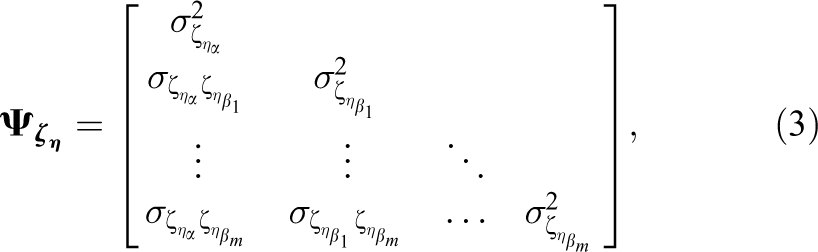
The most general covariance structure is UN. The unstructured covariance matrix of ∊ is given by

Θ_{∊} = [\begin{matrix} σ_{∊_{1}}^{2} \\ σ_{∊_{1} ∊_{2}} & σ_{∊_{2}}^{2} \\ ⋮ & ⋮ & ⋱ \\ σ_{∊_{1} ∊_{T}} & σ_{∊_{2} ∊_{T}} & \dots & σ_{∊_{T}}^{2} \end{matrix}] = [\begin{matrix} σ_{∊_{1}}^{2} \\ ρ_{∊_{1} ∊_{2}} σ_{∊_{1}} σ_{∊_{2}} & σ_{∊_{2}}^{2} \\ ⋮ & ⋮ & ⋱ \\ ρ_{∊_{1} ∊_{T}} σ_{∊_{1}} σ_{∊_{T}} & ρ_{∊_{2} ∊_{T}} σ_{∊_{2}} σ_{∊_{T}} & \dots & σ_{∊_{T}}^{2} \end{matrix}],

where $σ_{∊_{t}}^{2}$ is the variance of ∊_t at time point t, and $σ_{∊_{t} ∊_{t^{'}}}$ and $ρ_{∊_{t} ∊_{t^{'}}} = σ_{∊_{t} ∊_{t^{'}}} / (σ_{∊_{t}}^{} σ_{∊_{t^{'}}}^{})$ are, respectively, the autocovariance and autocorrelation of ∊_t and ∊_t′ at time points t and t′ (t ≠ t′). A simpler covariance structure may exist, which can be either stationary or non-stationary. An error process {∊_t} is stationary if the mean of ∊_t and the covariance of ∊_t and ∊_t−k, where k is an arbitrary integer, are both time-invariant (e.g., Box, Jenkins, & Reinsel, 1994, Ch. 3). More specifically, {∊_t} is stationary if (a) E(∊_t) = μ_∊ for all t, which is a constant, always assumed to be zero, and (b) $σ_{∊_{t}}^{2} = σ_{∊}^{2}$ for all t, and $σ_{∊_{t} ∊_{t^{'}}} = σ_{k}$ for all t, t′ satisfying |t − t′| = k, k > 0. That is, the variances are equal and the autocovariances at lag k are also equal, implying a constant autococorrelation at lag k, denoted by $ρ_{k} (= σ_{k} / σ_{∊}^{2})$ . Stationary structures include those resulting from the autoregressive and moving average process of order (p,q) [ARMA(p,q)], Toeplitz with q bands [TOEP(q)], q = 1, …, T (a constant variance, a constant correlation at lag k for 1 ≤ k ≤ q−1, and zero correlation at lag k for k ≥ q), and compound symmetry (CS) (a constant variance and a constant correlation regardless of the time lag). TOEP(T), simply denoted by TOEP, is the most general stationary structure. Non-stationary structures include heterogeneous TOEP(q) [TOEPH(q)] (non-constant variances, a constant correlation at lag k for 1 ≤ k ≤ q−1, and zero correlation at lag k for k ≥ q), heterogeneous CS (CSH) (non-constant variances and a constant correlation regardless of the time lag), heterogeneous AR(1) [ARH(1)] (non-constant variances and a constant autocorrelation between adjacent errors), the first order ante-dependence [ANTE(1)] (non-constant variances, non-constant correlations between adjacent errors, and assuming that the correlation between pairs of errors is the product of the correlations between adjacent times between them), and unstructured with q bands [UN(q)], q = 1, …, T (non-constant variances, non-constant correlation at lag k for 1 ≤ k ≤ q−1, and zero correlation at lag k for k ≥ q). TOEPH(T) and UN(T) are simply denoted by TOEPH and UN, respectively.

There are T(T + 1)/2 parameters [T variances and T(T −1)/2 autocorrelations] in UN. We summarize the parametric constraints placed on UN for different error covariance structures in Table 1. For each one, we show the constraints on autocorrelations, variances, or both and the number of parameters (reflecting the degree of parsimony). For example, for TOEP(T), the variances are constrained to be equal, and the autocorrelation at lag k is also constrained to be equal for 1 ≤ k ≤ T−1, so there are T parameters. For ARMA(1,1), there are three parameters (one constant variance, one autoregressive parameter φ₁, and one moving average parameter θ₁). The constant autocorrelation at lag k is further constrained by a specific relation through φ₁ and θ₁. Each covariance structure in the table was assigned a hypothesis number. When and how they are tested will be discussed in the next section.

Table 1.

Parametric constraints placed on UN for different level-1 error covariance structures

Covariance structure	Constraints	No. of para.	Hypothesis
Non-stationary
TOEPH(1)	$ρ_{∊_{t} ∊_{t^{'}}} = 0$	T	H₀₁
CSH	$ρ_{∊_{t} ∊_{t^{'}}} = ρ$	T + 1	H₀₂
ARH(1)	$ρ_{∊_{t} ∊_{t^{'}}} = ρ^{_{\| t - t^{'} \|}} = ρ^{_{k}}, \| t - t^{'} \| = k$	T + 1	H₀₃
TOEPH(q) (1<q<T)	$ρ_{∊_{t} ∊_{t^{'}}} = ρ_{k}, \| t - t^{'} \| = k < q; ρ_{∊_{t} ∊_{t^{'}}} = 0, \| t - t^{'} \| \geq q$	T + q –1	H₀₄
TOEPH	$ρ_{∊_{t} ∊_{t^{'}}} = ρ_{k}, \| t - t^{'} \| = k$	2T – 1	H₀₅
ANTE(1)	$ρ_{∊_{t} ∊_{t^{'}}} = \prod_{i = t}^{t^{'} - 1} ρ_{i}$	2T – 1	H₀₆
UN(q) (1< q < T)	$ρ_{∊_{t} ∊_{t^{'}}} = 0, \| t - t^{'} \| \geq q$	q(2T – q+1) /2	H₀₇
Stationary
TOEP(1)	$ρ_{∊_{t} ∊_{t^{'}}} = 0$ , $σ_{∊_{t}}^{2} = σ_{∊}^{2}$	1	$H_{01}^{'}$
CS	$ρ_{∊_{t} ∊_{t^{'}}} = ρ$ , $σ_{∊_{t}}^{2} = σ_{∊}^{2}$	2	$H_{02}^{'}$
AR(1)	$ρ_{∊_{t} ∊_{t^{'}}} = ρ_{k} = φ_{1}^{k}, \| t - t^{'} \| = k, σ_{∊_{t}}^{2} = σ_{∊}^{2}$	2	$H_{03}^{'}$
TOEP(q) (1< q < T)	$ρ_{∊_{t} ∊_{t^{'}}} = ρ_{k}, \| t - t^{'} \| = k < q; ρ_{∊_{t} ∊_{t^{'}}} = 0, \| t - t^{'} \| \geq q, σ_{∊_{t}}^{2} = σ_{∊}^{2}$	q	$H_{04}^{'}$
TOEP	$ρ_{∊_{t} ∊_{t^{'}}} = ρ_{k}, \| t - t^{'} \| = k$ , $σ_{∊_{t}}^{2} = σ_{∊}^{2}$	T	$H_{05}^{'}$
AR(2)	$ρ_{∊_{t} ∊_{t^{'}}} = ρ_{1} = φ_{1} / (1 - φ_{2}), \| t - t^{'} \| = 1,$ $ρ_{∊_{t} ∊_{t^{'}}} = ρ_{2} = φ_{1} ρ_{1} + φ_{2}, \| t - t^{'} \| = 2,$ $ρ_{∊_{t} ∊_{t^{'}}} = ρ_{k} = φ_{1} ρ_{k - 1} + φ_{2} ρ_{k - 2}, \| t - t^{'} \| = k > 2, σ_{∊_{t}}^{2} = σ_{∊}^{2}$	3	$H_{0a}^{'}$
ARMA(1,1)	$\begin{array}{l} ρ_{∊_{t} ∊_{t^{'}}} = ρ_{1} = \frac{(φ_{1} - θ_{1}) (1 - φ_{1} θ_{1})}{(1 - 2 φ_{1} θ_{1} + θ_{1}^{2})}, \| t - t^{'} \| = 1, \\ ρ_{∊_{t} ∊_{t^{'}}} = ρ_{k} = φ_{1} ρ_{k - 1}, \| t - t^{'} \| = k > 1, σ_{∊_{t}}^{2} = σ_{∊}^{2} \end{array}$	3	$H_{0b}^{'}$

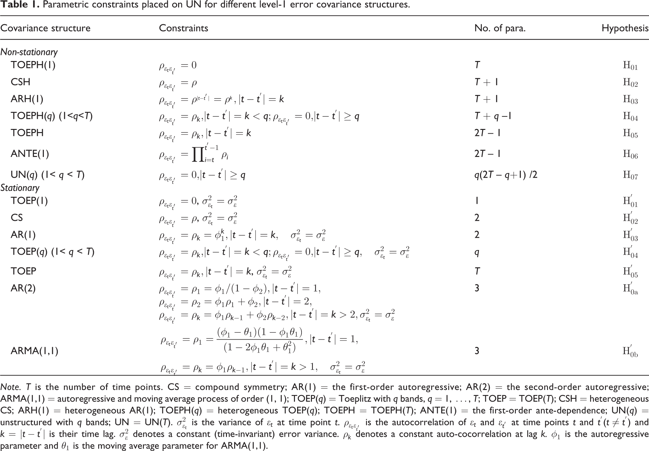
Note. T is the number of time points. CS = compound symmetry; AR(1) = the first-order autoregressive; AR(2) = the second-order autoregressive; ARMA(1,1) = autoregressive and moving average process of order (1, 1); TOEP(q) = Toeplitz with q bands, q = 1, …, T; TOEP = TOEP(T); CSH = heterogeneous CS; ARH(1) = heterogeneous AR(1); TOEPH(q) = heterogeneous TOEP(q); TOEPH = TOEPH(T); ANTE(1) = the first-order ante-dependence; UN(q) = unstructured with q bands; UN = UN(T). $σ_{∊_{t}}^{2}$ is the variance of ∊_t at time point t. $ρ_{∊_{t} ∊_{t^{'}}}$ is the autocorrelation of ∊_t and ∊_t′ at time points t and t′(t ≠ t′) and k = |t − t′| is their time lag. $σ_{∊}^{2}$ denotes a constant (time-invariant) error variance. ρ_k denotes a constant auto-cocorrelation at lag k. φ₁ is the autoregressive parameter and θ₁ is the moving average parameter for ARMA(1,1).

The nested relations among the error covariance structures are easy to obtain based on the constraints placed on UN summarized in Table 1. They are explicitly presented with a tree diagram in Figure 1 (by following Widaman and Thompson, 2003). In this article, p* and q* are used to represent the order of the ARMA process to distinguish from the q in TOEP(q), TOEPH(q), and UN(q). Note that AR(p*) = ARMA(p*,0) and MA(q*) = ARMA(0,q*). Because the model fit with MA(q*) and that with TOEP(q*+1) are identical, MA(q*) is ignored. In Figure 1, stationary and non-stationary structures are separated with a horizontal dashed line. Stationary structures appear below the line and non-stationary ones above the line. The lines with single-headed arrow connect two covariance structures from a more constrained one to a less constrained one in such a way that the former is nested within the latter. The constraints are indicated beside the lines. For example, TOEPH(1) is nested within CSH as well as within ARH(1) by the constraint of ρ = 0. CS is nested within TOEP by the constraint of ρ_k = ρ. 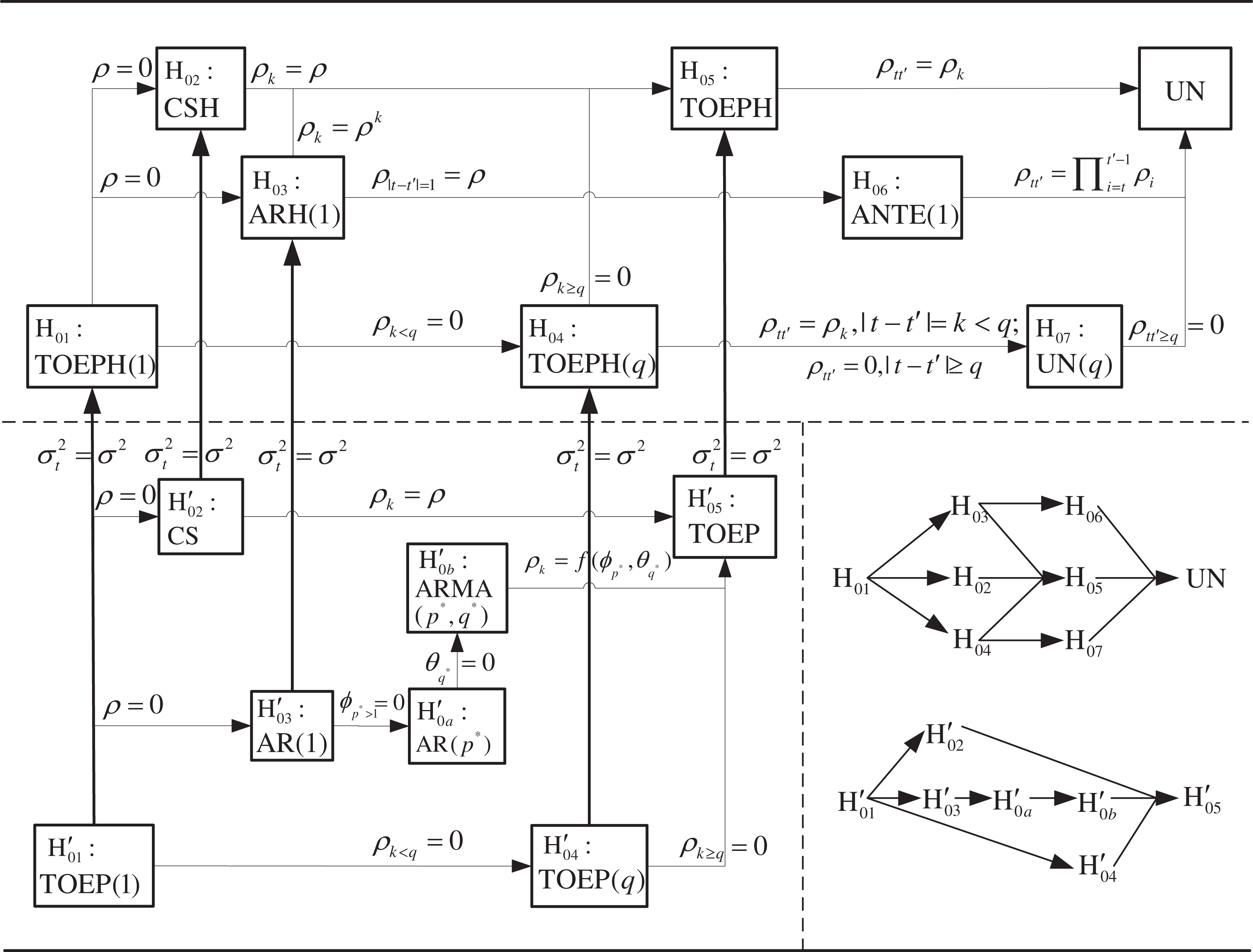The vertical lines through the dashed line indicate the constraint of invariant variance (i.e., $σ_{∊_{t}}^{2} = σ_{∊}^{2}$ ), by which the non-stationary structures reduce to the stationary ones. For example, TOEP(2) is nested within TOEPH(2) and AR(1) is nested within ARH(1).

Figure 1.

Tree diagram showing the nested relations among the level-1 error covariance structures based on the constraints placed

UN is called the saturated structure and TOEP is called the saturated stationary structure. TOEPH(1) and TOEP(1) are the simplest (the most constrained) non-stationary and stationary structures, respectively. For non-stationary structures, TOEPH(1) is nested within CSH, ARH(1), and TOEPH(q), ARH(1) is nested within TOEPH and ANTE(1), TOEPH(q) is nested within TOEPH and UN(q), and they are all nested within UN. For stationary structures, TOEP(1) is nested within CS, AR(1), and TOEP(2). AR(1) is nested within AR(p*), which is nested within ARMA(p*,q*). They are all nested within TOEP. The nested relationships among the structures are simplified in the lower right corner of Figure 1. Note that there exists no nested relation for the structures in each of the sets of {CS, ARMA(p*,q*)}, {TOEP(q), AR(p*)}, and {CSH, ARH(1), TOEPH(q)}.

A systematic approach for identifying level-1 error covariance structures

In this section, a systematic approach is proposed to search for a plausible level-1 error covariance structure. The approach is then evaluated by two simulation studies with the linear growth model, one of which is based on a non-stationary level-1 covariance structure, and the other is based on a stationary covariance structure. The approach is finally illustrated with empirical data.

Because the error covariance structures shown in Figure 1 are all nested within UN, the chi-square difference test (Bollen & Curran, 2006, p. 51) can be used to test the adequacy for each of them by assessing if the resulting model fit is not significantly worse than that from the saturated structure UN. Moreover, all stationary structures are also nested within TOEP, so the chi-square difference test can also be conducted based on the saturated stationary structure TOEP. The latter test facilitates identifying a simple plausible structure. Note that TOEP is nested within UN, and therefore the chi-square difference test can also be used to test stationarity of the level-1 error covariance structure.

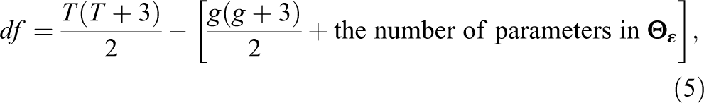
Before we conduct the chi-square difference test, we need to examine the condition for model identification. The unknown parameters in an unconditional growth model include Γ ₀, $Ψ_{ζ_{η}}$ , and Θ _∊. One necessary condition for model identification, assuming that $Ψ_{ζ_{η}}$ = UN, is that the degrees of freedom (df) given below is positive (Bollen & Curran, 2006, p. 23):

d f = \frac{T (T + 3)}{2} - [\frac{g (g + 3)}{2} + the number of parameters in Θ_{∊}],

where g denotes the number of growth parameters. The df for the model with Θ _∊= UN, TOEPH, and TOEP based on Equation 5, are T − g(g + 3)/2 and [T(T −1) + 2]/2 − g(g + 3)/2, and T(T +1)/2 − g(g + 3)/2, respectively. Table 2 summarizes the minimum numbers of time points required to achieve model identification for the linear, quadratic, and cubic growth models with $Ψ_{ζ_{η}}$ = UN and Θ _∊= UN, TOEPH, or TOEP.

Table 2.

The minimum number of time points required to achieve model identification for the unconditional linear, quadratic, and cubic growth models with $Ψ_{ζ_{η}}$ = UN and Θ _∊= UN, TOEPH or TOEP

Growth model (g)	Θ _∊	The minimum T required
Linear (2)	UN (non-stationary)	6
	TOEPH (non-stationary)	4
	TOEP (stationary)	3
Quadratic (3)	UN (non-stationary)	10
	TOEPH (non-stationary)	5
	TOEP (stationary)	4
Cubic (4)	UN (non-stationary)	15
	TOEPH (non-stationary)	6
	TOEP (stationary)	5

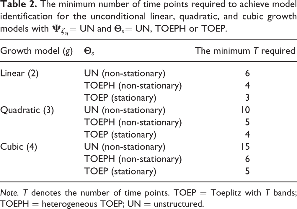
Note. T denotes the number of time points. TOEP = Toeplitz with T bands; TOEPH = heterogeneous TOEP; UN = unstructured.

The search procedure for a level-1 error covariance structure consists of two stages:

Stage 1: Testing the stationarity of a level-1 error covariance structure.

For the linear growth model (g = 2) with $Ψ_{ζ_{η}}$ = UN and Θ _∊= UN, the least value of T to produce a positive df is 6. For T = 6, the null hypothesis for stationarity is given by placing the following constraints on UN:

H_{0} : {\begin{matrix} \begin{array}{l} σ_{∊_{1}}^{2} = σ_{∊_{2}}^{2} = σ_{∊_{3}}^{2} = σ_{∊_{4}}^{2} = σ_{∊_{5}}^{2} = σ_{∊_{6}}^{2}, \\ σ_{∊_{1} ∊_{2}} = σ_{∊_{2} ∊_{3}} = σ_{∊_{3} ∊_{4}} = σ_{∊_{4} ∊_{5}} = σ_{∊_{5} ∊_{6}}, \\ σ_{∊_{1} ∊_{3}} = σ_{∊_{2} ∊_{4}} = σ_{∊_{3} ∊_{5}} = σ_{∊_{4} ∊_{6}}, \end{array} \\ \begin{array}{l} σ_{∊_{1} ∊_{4}} = σ_{∊_{2} ∊_{5}} = σ_{∊_{3} ∊_{6}}, \\ σ_{∊_{1} ∊_{5}} = σ_{∊_{2} ∊_{6}} . \end{array} \end{matrix}

The df associated with the test for stationarity by using the saturated structure UN is T(T −1)/2. When T < 6 and Θ _∊= UN, model identification fails. For T = 4, TOEPH is selected as the least constrained structure instead of UN for the chi-square difference test because, when g = 2, the corresponding df = 2 > 0. The constraints on TOEPH for stationarity become

H_{0} : σ_{∊_{1}}^{2} = σ_{∊_{2}}^{2} = σ_{∊_{3}}^{2} = σ_{∊_{4}}^{2} .

The df associated with the test for stationarity by using TOEPH as the least constrained structure is T −1. Under stationarity, UN and TOEPH both reduce to TOEP, the saturated stationary structure. Although, for T = 4, UN(2) and ANTE(1) could also achieve model identification (df > 0), neither of them is considered because, under stationarity, they cannot reduce to TOEP (see Figure 1), on which the subsequent search procedure for a more parsimonious stationary structure is based. In fact, they reduce to TOEP(2) and AR(1), respectively, both nested within TOEP.

The ways for handling the quadratic or higher-order growth model are similar.

Stage 2: Identifying a plausible level-1 error covariance structure.

If stationarity, tested in Stage 1, is supported, then identify the structure within the stationary group; otherwise identify the structure within the non-stationary group. The search procedure, shown in Figure 2 with a flowchart, basically follows the sequential chi-square difference test (SCDT) given by Anderson and Gerbing (1988). The structure to be identified is as simple as possible under the condition that it is nested within the least constrained structure and it produces no significantly worse model fit than the least constrained structure. Structure search is conducted sequentially, starting from the simplest (i.e., the most constrained) model and then a less constrained one. The process is terminated when the test becomes nonsignificant. If there exist two or more equally parsimonious structures, they all need to be compared with the least constrained structure used.

Figure 2.

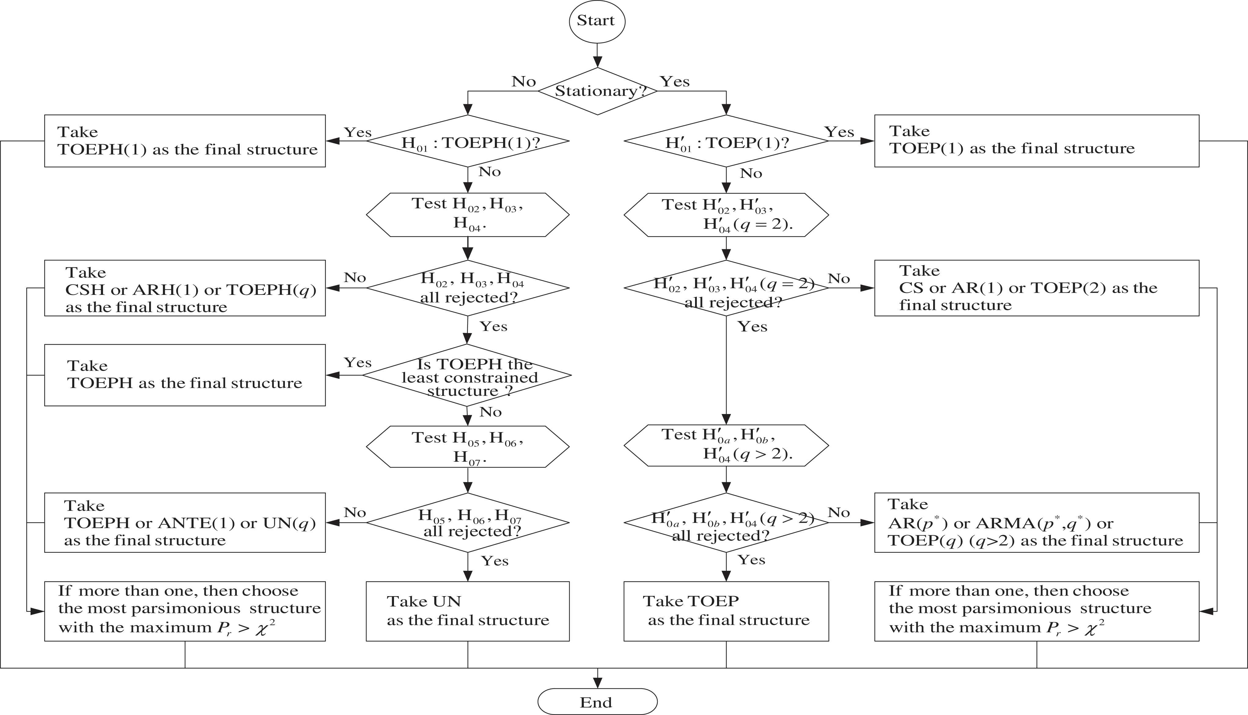
Flowchart for identifying a plausible level-1 error covariance structure

Stationarity holds

The procedure to search for a plausible stationary structure, shown on the right side of Figure 2, starts from testing $H_{01}^{'}$ : TOEP(1). The least constrained structure used is TOEP. If $H_{01}^{'}$ is not rejected, then take TOEP(1) as the final structure and stop the procedure; otherwise test $H_{02}^{'}$ : CS, $H_{03}^{'}$ : AR(1), and $H_{04}^{'}$ : TOEP(2), and take those showing nonsignificance. If CS, AR(1), and TOEP(2) are all rejected, then test $H_{0 a}^{'}$ : AR(p*), $H_{0 b}^{'}$ : ARMA(p*,q*), and $H_{04}^{'}$ : TOEP(q)(q > 2). For $H_{0 a}^{'}$ , the test is carried out sequentially, starting from AR(2). If the test for AR(p*) is nonsignificant, we stop the process by returning the most parsimonious AR(p*). For $H_{0 b}^{'}$ , according to the degree of parsimony, the ARMA(p*,q*) processes to be examined are in the order of ARMA(1,1), [ARMA(2,1), ARMA(1,2)], [ARMA(3,1), ARMA(2,2), ARMA(1,3)], …, and [ARMA(p*,q*), p*+q* = T−2]. The processes within the same parenthesis are those with the same number of parameters. ARMA(p*,q*), p*+q* = T−1, are not candidates because they have the same number of parameters as TOEP, leading to zero degree of freedom for the chi-square difference test. Again, the search process stops when nonsignificance occurs. For $H_{04}^{'}$ : TOEP(q) (q > 2), the value of q is also determined by the same principle. If two or more structures show nonsignificance, choose the most parsimonious one. If $H_{0 a}^{'}$ , $H_{0 b}^{'}$ , and $H_{04}^{'}$ are all rejected, take TOEP as the final choice.

b. Stationarity does not hold

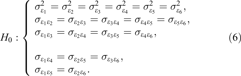
The procedure to search for a plausible non-stationary structure, shown on the left side of Figure 2, starts from testing H₀₁: TOEPH(1). When T is large enough, use UN as the least constrained structure; otherwise use TOEPH. If H₀₁ is not rejected, then take TOEPH(1) as the final structure; otherwise test H₀₂: CSH, H₀₃: ARH(1), and H₀₄: TOEPH(q) (q = 2, …, T−1). Starting from TOEPH(2), we test H₀₄ sequentially until the occurrence of nonsignificance, thereby determining the value of q. If the tests for q = 2, …, T−1, are all significant, then H₀₄ is rejected. If two or all of CSH, ARH(1), and TOEPH(q) do not show significantly worse model fit, choose the structure with the least parameters. If H₀₂, H₀₃, and H₀₄ are all rejected, check if TOEPH is used as the least constrained structure. If it is, then take it as the final structure; otherwise test H₀₅: TOEPH, H₀₆: ANTE(1), and H₀₇: UN(q) (q = 2, …,T−1). The value of q for H₀₇ is also determined by the same principle as above. If H₀₅, H₀₆, and H₀₇ are not all rejected, then choose the most parsimonious one from those showing nonsignificance; otherwise take UN as the final choice.

During the search procedure, if there exist two or more structures with the same number of parameters and with no significant difference in model fit from the least constrained structure, then choose the one with the largest p value of the chi-square test (e.g., de la Torre, van der Ark, & Rossi, 2015). Whenever comparing models that are not nested, model selection indices such as AIC and BIC can be used. When the structures have the same number of parameters, AIC and BIC will lead to the same result as the p value. Note that the procedure and the corresponding flow chart apply to the cases where T ≥ 4. When T = 3, TOEPH(1) is the only non-stationary structure that can achieve model identification for the zunconditional linear growth model, and therefore it is used as the least constrained non-stationary structure in this case. However, TOEP, the saturated stationary structure, is not nested within TOEPH(1). The constraints on TOEPH(1) for stationarity are given by $σ_{∊_{1}}^{2} = σ_{∊_{2}}^{2} = σ_{∊_{3}}^{2}$ , leading TOEPH(1) to TOEP(1). Therefore, stationarity can only be tested by comparing TOEP(1) and TOEPH(1) using the chi-square difference test with 2 df. If the test is significant, then take TOEPH(1) as the final structure; otherwise proceed to compare TOEP(1) with TOEP because TOEP can also be identified when T = 3. If TOEP(1) is not significantly worse than TOEP in model fit, then take TOEP(1) as the final structure; otherwise compare CS, AR(1), and TOEP(2) with TOEP. If CS, AR(1), and TOEP(2) are not all significantly worse than TOEP in model fit, then choose the one with the largest p value; otherwise take TOEP to be the final choice.

Simulation

We conducted two simulation studies to assess the performance of the proposed approach. Although AR(1) may be the most commonly used one to capture the level-1 error correlations (Murphy & Pituch, 2009, p. 256), ARH(1) is more appropriate when error variances and autocovariances are not homogeneous. Therefore, ARH(1) and AR(1), representing a non-stationary structure and a stationary one, respectively, were selected for Θ _∊, coupled with UN for $Ψ_{ζ_{η}}$ , in the simulation studies. In each study, 1000 replications were generated for each of the sample sizes (denoted by N) of 150, 300, and 500 (Ding & Jane, 2012; Ferron et al., 2002) from the population linear growth model. According to Kwok et al. (2007), among the multiwave longitudinal studies published in Developmental Psychology in 2002, more than half (52%) of these studies collected data with three or four occasions. However, as shown in Table 2, the minimum values of T to achieve model identification for the linear growth model with Θ _∊= UN and TOEPH are 6 and 4, respectively. Hence, Study 1 is based on the population model with Θ _∊= ARH(1) and T = 6, and Study 2 is based on that with Θ _∊ = AR(1) and T = 4. The test for stationarity can be conducted by using UN as the least constrained structure in Study 1 and by using TOEPH in Study 2. Because the effects of Θ _∊ and $Ψ_{ζ_{η}}$ of different magnitudes are not of concern, single values were used for them. By following Ding and Jane (2012), the population parameter values in Study 1 were set as γ₀₀ = 10, γ01 = 4, $σ_{ζ_{η_{α}}}^{2}$ = 15, $σ_{ζ_{η_{β_{1}}}}^{2}$ = 10, $σ_{ζ_{η_{α}} ζ_{η_{β_{1}}}} = 7,$ $σ_{∊_{1}}^{2} = 36,$ $σ_{∊_{2}}^{2} = 25,$ $σ_{∊_{3}}^{2} = 49,$ $σ_{∊_{4}}^{2} = 64,$ $σ_{∊_{5}}^{2} = 25,$ and $σ_{∊_{6}}^{2} = 36.$ The levels for ρ in ARH(1) include 0.7, 0.5, 0.2, and 0. The first three levels of the autocorrelation are more representative than those used in Ferron et al. (2002). The ARH(1) with ρ = 0 is actually TOEPH(1). Regarding the population parameters in Study 2, we used the same values of growth parameters and autocorrelations as above. Error variances/covariances were arbitrarily set as $σ_{ζ_{η_{α}}}^{2}$ = 4, $σ_{ζ_{η_{β_{1}}}}^{2}$ = 1, $σ_{ζ_{η_{α}} ζ_{η_{β_{1}}}}$ = −1, and $σ_{∊}^{2} = 4$ . The 0.05 level of significance was used for each test encountered.

An effective replication is defined as one with convergent and proper solutions. The percentage of effective replications out of 1000 was examined in each study. We then calculated the relative frequencies of the level-1 error covariance structures identified by the proposed approach out of effective replications. The percentage of the agreement between the covariance structure identified and the population structure is the rate of correct identification, which is used to evaluate the effectiveness of the proposed approach in recovering the correct covariance structure.

The relative biases of parameter estimates resulting from fitting different level-1 error covariance structures were also examined. The relative bias of each parameter estimate ${\hat{θ}}_{j}$ is defined as (Hoogland & Boomsma, 1998)

R B ({\hat{θ}}_{j}) = (\bar{{\hat{θ}}_{j}} - θ_{j}) / θ_{j},

where θ_j is the population value of the _jth parameter (θ_j ≠ 0), and $\bar{{\hat{θ}}_{j}}$ is the mean of the parameter estimates across effective simulation replications. The criterion for acceptability is | $R B ({\hat{θ}}_{j})$ | < 5%.

Misspecifications in LGM come from the mean, covariance, or both structures. The covariance structure is the combination of the level-1 and level-2 error covariance matrices. Wu, West, and Taylor (2009) indicated that, for balanced designs with complete data, RMSEA, CFI, and TLI among the SEM-based fit indices have shown good potential performance in evaluating the fit in both mean and covariance structures. In addition, SRMR is more sensitive to misspecification in the covariance structure than to the misspecification in the mean structure. Since it is assumed that there exists no misspecification in the mean structure and the level-2 error covariance structure is unconstrained (saturated), any misfit is due to the level-1 error covariance structure. Under these conditions, RMSEA, CFI, TLI, and SRMR can be considered. RMSEA, CFI, and TLI are chi-square-based fit indices. They are not included because the p value associated with chi-square test for model fit (denoted by P_r > χ²) has been reported. Instead, SRMR, a residual-based fit index, is used.

Simulation was implemented by using SAS. SAS codes by PROC CALIS to fit various level-1 error covariance structures are available in Ding and Jane (2012). The simulation results are summarized in Table 3 and Table 4 (for Study 1) and Table 5 and Table 6 (for Study 2). In Study 1, when ρ = 0.7, the number of effective replications out of 1000 was 945 for N = 150, 993 for N = 300, and 995 for N = 500 (see Table 3). Of the effective replications, the proportion of rejecting stationarity was found to be 100%, regardless of the sample size. In each replication, we followed the procedure shown on the left side of Figure 2 to identify a non-stationary level-1 error covariance structure. TOEPH(1) was rejected in all replications. As shown in the table, the frequencies of correctly identifying ARH(1) were 850, 971, and 995 for N = 150, 300, and 500, respectively. Therefore, the relative frequencies (i.e., the rates of correct identification) were 89.95%, 97.78%, and 100%. On the other hand, the relative frequency of incorrectly identifying TOEPH(2) was 8.68% when N = 150, and was reduced to 1.01% when N = 300. CSH was not identified. ARH(1) and TOEPH(2) were the most parsimonious identified structures and they together occupied the majority. Other structures, which were non-stationary and less parsimonious, were ascribed to the category of “Others,” whose relative frequency was 1.37% when N = 150 and 1.21% when N = 300.

Table 3.

Simulation results based on ARH(1) for different sample sizes (Part A)

N	No. of effective replications	Structure identified	Frequency (Relative freq. [%])	Model fit
N	No. of effective replications	Structure identified	Frequency (Relative freq. [%])	$\bar{P_{r} > χ^{2}}$	$\bar{SRMR}$
(1) For ρ= 0.7:
150	945	ARH(1)	850 (89.95)	0.500	0.032
		TOEPH(2)	82 (8.68)	0.146	0.029
		Others	13 (1.37)	–	–
300	993	ARH(1)	971 (97.78)	0.498	0.021
		TOEPH(2)	10 (1.01)	0.154	0.030
		Others	12 (1.21)	–	–
500	995	ARH(1)	995 (100.00)	0.542	0.016
		Others	0 (0.00)	–	–
(2) For ρ= 0.5:
150	950	ARH(1)	705 (74.21)	0.520	0.033
		TOEPH(2)	221 (23.26)	0.376	0.034
		TOEPH(1)	16 (1.68)	0.074	0.032
		Others	8 (0.84)	–	–
300	980	ARH(1)	925 (94.39)	0.534	0.023
		TOEPH(2)	48 (4.90)	0.264	0.024
		Others	7 (0.71)	–	–
500	997	ARH(1)	973 (97.59)	0.504	0.021
		Others	24 (2.41)	–	–
(3) For ρ= 0.2:
150	974	ARH(1)	118 (12.11)	0.345	0.042
		TOEPH(2)	113 (11.60)	0.346	0.038
		TOEPH(1)	720 (73.92)	0.242	0.043
		Others	23 (2.36)	–	–
300	985	ARH(1)	385 (39.09)	0.510	0.029
		TOEPH(2)	280 (28.43)	0.492	0.030
		TOEPH(1)	313 (31.78)	0.128	0.029
		Others	7 (0.71)	–	–
500	998	ARH(1)	543 (54.41)	0.501	0.022
		TOEPH(2)	384 (38.48)	0.520	0.023
		TOEPH(1)	60 (6.01)	0.103	0.023
		Others	11 (1.10)	–	–
(4) For ρ= 0:
150	993	TOEPH(1)	960 (96.68)	0.490	0.045
		Others	33 (3.32)	–	–
300	1000	TOEPH(1)	987 (98.70)	0.470	0.032
		Others	13 (1.30)	–	–
500	1000	TOEPH(1)	985 (98.50)	0.505	0.025
		Others	15 (1.50)	–	–

Note. The number of replications is 1000. ARH(1) = heterogeneous first-order autoregressive; TOEPH(1) = heterogeneous Toeplitz with 1 band; TOEPH(2) = heterogeneous Toeplitz with 2 bands. The ARH(1) with ρ = 0 is actually TOEPH(1).

Table 4.

Simulation results based on ARH(1) for different sample sizes (Part B)

N	No. of effective replications	Structure specified	Model fit		Relative bias [%]
N	No. of effective replications	Structure specified	$\bar{P_{r} > χ^{2}}$	$\bar{SRMR}$	${\hat{γ}}_{00}$	${\hat{γ}}_{01}$	${\hat{σ}}_{ζ_{η_{α}}}^{2}$	${\hat{σ}}_{ζ_{η_{β}}}^{2}$	${\hat{σ}}_{ζ_{η_{α}} ζ_{η_{β}}}$	${\hat{σ}}_{∊_{1}}^{2}$	${\hat{σ}}_{∊_{2}}^{2}$	${\hat{σ}}_{∊_{3}}^{2}$	${\hat{σ}}_{∊_{4}}^{2}$	${\hat{σ}}_{∊_{5}}^{2}$	${\hat{σ}}_{∊_{6}}^{2}$	$\hat{ρ}$
(1) For ρ= 0.7:
150	945	ARH(1)	0.493	0.034	0.03	0.19	1.09	0.47	−1.20	0.40	−1.27	2.01	0.87	1.03	−1.67	0.68
		TOEPH(2)	0.054	0.047	−0.05	0.12	123.50	11.20	−39.82	−55.37	−58.27	−50.00	−47.08	−60.15	−53.80	0.38
300	993	ARH(1)	0.491	0.025	−0.18	−0.19	−1.82	−0.61	−0.23	0.95	1.41	0.46	0.68	0.81	−0.73	0.68
		TOEPH(2)	0.047	0.040	−0.20	−0.25	138.48	18.18	−45.04	−49.68	−60.45	−52.97	−48.7	−52.61	−48.27	0.40
500	995	ARH(1)	0.542	0.016	0.05	0.12	−3.84	−0.08	0.46	0.81	1.34	0.98	0.75	1.63	0.65	0.78
(2) For ρ= 0.5:
150	950	ARH(1)	0.510	0.037	−0.05	0.08	2.10	−0.03	−0.66	0.76	1.02	1.95	1.40	−1.08	0.29	0.50
		TOEPH(2)	0.309	0.040	−0.04	0.07	78.61	6.82	−35.02	−28.02	−28.10	−24.24	−25.68	−43.60	−22.39	0.30
		TOEPH(1)	0.001	0.049	0.07	0.03	118.85	19.14	−60.52	−40.62	−50.44	−32.91	−37.21	−60.95	−28.01	–
300	980	ARH(1)	0.516	0.026	−0.05	0.35	−3.31	0.34	2.80	1.62	2.25	2.35	1.02	1.05	0.79	0.49
		TOEPH(2)	0.167	0.032	−0.07	0.36	87.30	7.70	−27.63	−30.87	−31.05	−24.15	−23.71	−34.06	−23.25	0.29
500	997	ARH(1)	0.504	0.021	−0.07	0.06	−3.87	0.36	1.88	1.65	1.80	1.45	1.25	0.62	1.25	0.40
(3) For ρ= 0.2:
150	974	ARH(1)	0.501	0.045	−0.15	−0.03	1.78	0.41	1.04	0.42	−0.52	0.41	1.28	−0.61	2.03	0.20
		TOEPH(2)	0.490	0.040	−0.13	−0.03	15.36	2.25	−5.35	−5.35	−5.01	−4.75	−6.14	−6.98	1.74	0.16
		TOEPH(1)	0.185	0.045	−0.16	−0.02	53.21	9.03	−24.67	−17.45	−26.58	−7.69	−8.72	−27.50	−5.17	–
300	985	ARH(1)	0.472	0.035	0.00	0.03	−2.17	−0.68	1.21	0.09	0.29	−0.18	1.10	3.08	3.00	0.71
		TOEPH(2)	0.470	0.035	0.01	0.03	12.35	0.89	−6.09	−4.83	−5.50	−4.47	−3.35	−2.96	−0.60	0.15
		TOEPH(1)	0.045	0.034	−0.02	0.02	52.56	7.00	−20.52	−16.21	−24.19	−9.10	−10.47	−21.84	−6.88	–
500	998	ARH(1)	0.480	0.025	0.04	0.24	−1.82	0.00	0.20	0.64	−0.27	0.07	0.63	1.92	1.19	0.19
		TOEPH(2)	0.481	0.028	0.04	0.23	10.94	1.87	−5.72	−4.63	−5.75	−3.57	−3.76	−3.58	−1.20	0.17
		TOEPH(1)	0.006	0.029	0.04	0.25	53.17	8.24	−27.01	−19.17	−20.19	−8.98	−12.26	−22.06	−6.00	–
(4) For ρ= 0:
150	993	TOEPH(1)	0.485	0.047	0.14	0.38	−1.23	−0.41	2.08	2.98	3.07	2.17	2.24	−4.45	3.54	–
300	1000	TOEPH(1)	0.468	0.036	−0.02	0.04	−2.50	−0.98	1.50	1.21	2.09	1.98	2.06	−4.01	3.95	–
500	1000	TOEPH(1)	0.501	0.028	0.05	−0.26	−3.32	−0.34	0.40	1.08	3.55	2.11	1.87	−3.11	2.99	–

Table 5.

Simulation results based on AR(1) for different sample sizes (Part A)

N	No. of effective replications	Structure identified	Frequency (Relative freq. [%])	Model fit
N	No. of effective replications	Structure identified	Frequency (Relative freq. [%])	$\bar{P_{r} > χ^{2}}$	$\bar{SRMR}$
(1) For ρ= 0.7:
150	750	AR(1)	253 (33.73)	0.630	0.022
		TOEP(2)	215 (28.67)	0.603	0.025
		TOEP(1)	230 (30.67)	0.310	0.030
		Others	52 (6.93)	–	–
300	810	AR(1)	511 (63.09)	0.608	0.016
		TOEP(2)	216 (26.67)	0.582	0.018
		TOEP(1)	15 (1.85)	0.248	0.021
		Others	68 (8.40)	–	–
500	867	AR(1)	635 (73.24)	0.573	0.013
		TOEP(2)	168 (19.38)	0.579	0.014
		Others	64 (7.38)	–	–
(2) For ρ= 0.5:
150	852	AR(1)	241 (28.29)	0.640	0.029
		TOEP(2)	228 (26.76)	0.587	0.024
		TOEP(1)	330 (38.73)	0.309	0.040
		Others	53 (6.22)	–	–
300	950	AR(1)	520 (54.74)	0.568	0.022
		TOEP(2)	263 (27.68)	0.623	0.023
		TOEP(1)	65 (6.84)	0.256	0.029
		Others	102 (10.74)	–	–
500	973	AR(1)	640 (65.78)	0.562	0.017
		TOEP(2)	251 (25.80)	0.600	0.017
		Others	82 (8.42)	–	–
(3) For ρ= 0.2:
150	975	TOEP(1)	766 (78.56)	0.476	0.046
		AR(1)	38 (3.90)	0.599	0.037
		TOEP(2)	57 (5.85)	0.587	0.044
		Others	114 (11.69)	–	–
300	992	TOEP(1)	650 (65.52)	0.430	0.033
		AR(1)	128 (12.90)	0.537	0.028
		TOEP(2)	112 (11.29)	0.601	0.029
		Others	102 (10.28)	–	–
500	999	TOEP(1)	460 (46.05)	0.367	0.026
		AR(1)	221 (22.12)	0.576	0.022
		TOEP(2)	210 (21.02)	0.602	0.022
		Others	108 (10.81)	–	–

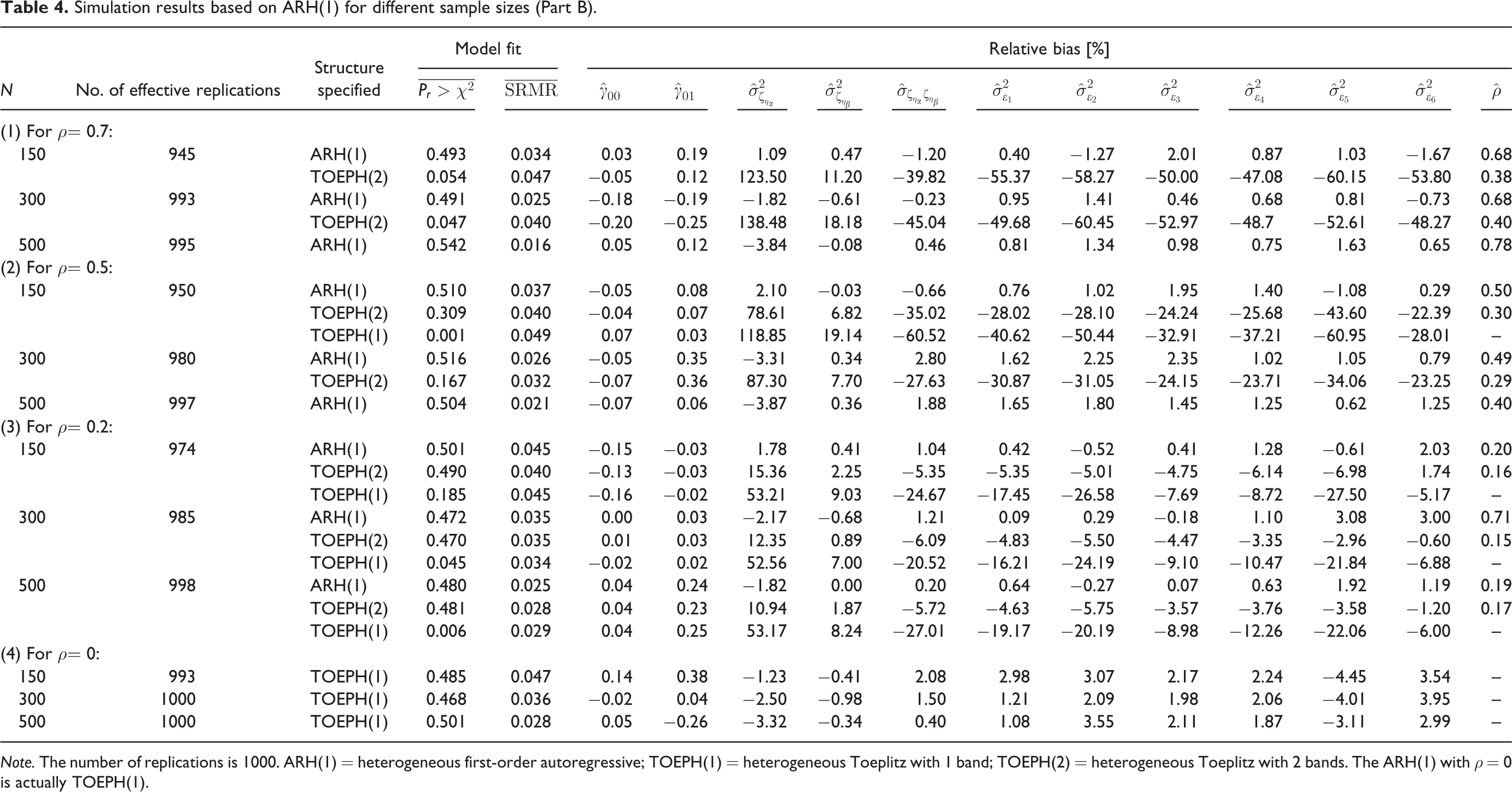
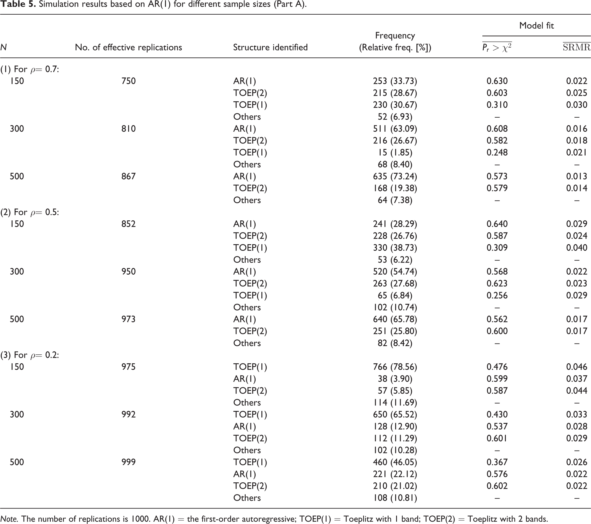
Note. The number of replications is 1000. AR(1) = the first-order autoregressive; TOEP(1) = Toeplitz with 1 band; TOEP(2) = Toeplitz with 2 bands.

Table 6.

Simulation results based on AR(1) for different sample sizes (Part B)

N	No. of effective replications	Structure specified	Model fit		Relative bias [%]
N	No. of effective replications	Structure specified	$\bar{P_{r} > χ^{2}}$	$\bar{SRMR}$	${\hat{γ}}_{00}$	${\hat{γ}}_{01}$	${\hat{σ}}_{ζ_{η_{α}}}^{2}$	${\hat{σ}}_{ζ_{η_{β}}}^{2}$	${\hat{σ}}_{ζ_{η_{α}} ζ_{η_{β}}}$	${\hat{σ}}_{∊_{1}}^{2}$	$\hat{ρ}$
For ρ= 0.7:
150	750	AR(1)	0.529	0.026	−0.04	0.04	6.40	4.58	4.40	−4.17	−4.80
		TOEP(2)	0.525	0.028	−0.05	0.04	64.67	22.77	30.56	−60.15	−57.31
		TOEP(1)	0.117	0.034	−0.04	0.04	79.25	39.18	52.17	−75.01	–
300	810	AR(1)	0.520	0.018	−0.06	−0.05	5.01	4.22	4.36	−2.07	−4.52
		TOEP(2)	0.441	0.023	−0.06	−0.03	65.66	23.24	35.15	−58.20	−50.71
		TOEP(1)	0.014	0.032	−0.06	−0.04	81.57	39.25	57.40	−72.92	–
500	867	AR(1)	0.504	0.014	−0.03	−0.02	3.16	3.01	4.94	−2.04	−3.50
		TOEP(2)	0.324	0.022	−0.01	−0.01	64.50	25.65	34.88	−58.46	−51.46
(2) For ρ= 0.5:
150	852	AR(1)	0.502	0.035	−0.12	−0.20	1.80	3.50	1.41	−4.07	−0.11
		TOEP(2)	0.503	0.037	0.14	−0.12	37.22	18.50	32.50	−35.39	−39.40
		TOEP(1)	0.149	0.045	0.13	−0.17	52.98	41.89	71.20	−50.16	–
300	950	AR(1)	0.504	0.024	0.03	−0.06	−2.26	1.65	2.63	3.26	−4.01
		TOEP(2)	0.440	0.029	0.02	−0.08	37.65	24.54	31.66	−33.20	−44.25
		TOEP(1)	0.030	0.042	0.03	−0.07	59.89	42.58	62.42	−50.28	–
500	973	AR(1)	0.490	0.019	−0.03	−0.03	−4.70	−1.12	−1.58	4.27	−0.54
		TOEP(2)	0.378	0.025	−0.01	−0.03	39.09	19.74	28.70	−33.15	−40.56
(3) For ρ= 0.2:
150	975	TOEP(1)	0.406	0.049	−0.15	0.14	25.01	23.96	36.98	−20.20	–
		AR(1)	0.535	0.043	−0.13	0.13	−2.28	−0.50	0.94	3.35	−1.09
		TOEP(2)	0.536	0.044	−0.12	0.11	6.69	7.99	11.15	−8.05	−32.19
300	992	TOEP(1)	0.308	0.037	0.01	0.05	23.65	22.25	33.51	−20.14	–
		AR(1)	0.527	0.030	0.02	−0.10	0.41	−0.14	1.79	0.59	0.02
		TOEP(2)	0.523	0.031	0.01	0.07	7.08	6.89	9.10	−6.12	−23.02
500	999	TOEP(1)	0.193	0.032	0.03	−0.02	26.61	22.95	33.20	−20.78	–
		AR(1)	0.530	0.024	0.03	−0.03	−0.71	0.31	0.57	1.17	0.24
		TOEP(2)	0.519	0.025	0.04	−0.02	6.89	5.66	9.11	−5.35	−23.21

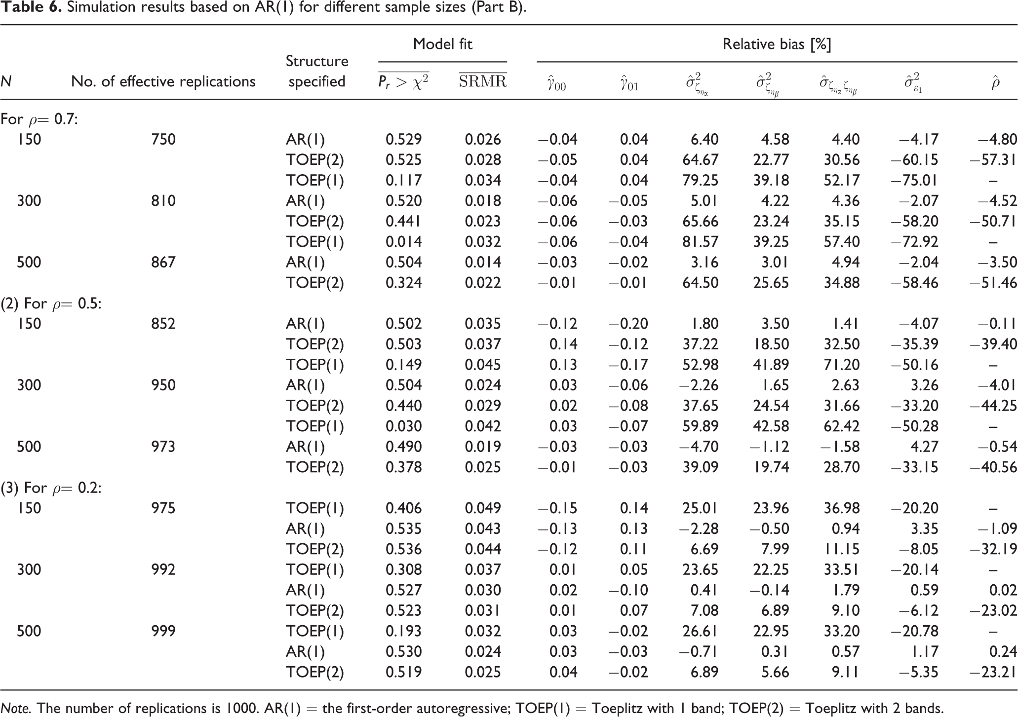
Note. The number of replications is 1000. AR(1) = the first-order autoregressive; TOEP(1) = Toeplitz with 1 band; TOEP(2) = Toeplitz with 2 bands.

When ρ = 0.5 or 0.2, the percentages of effective replications were also high (at least 95%). Although the proportions of rejecting stationarity were still large (close to 100%) for all cases, the rate of correct identification was much reduced when N = 150 (74.21% for ρ = 0.5 and 12.11% for ρ = 0.2). When ρ is low, the difference among ARH(1), TOEPH(2), and TOEPH(1) is not salient, so ARH(1) becomes difficult to identify. However, misidentification can be improved by using larger sample sizes. When ρ = 0, ARH(1) is actually TOEPH(1), and the replications were almost all effective. The rates of correctly identifying TOEPH(1) were greater than 96%.

In Table 3, the model fit, reported based on the means of P_r > χ² and SRMR (denoted by $\bar{P_{r} > χ_{}^{2}}$ and $\bar{SRMR}$ ), was satisfactory in each case. For each case, we further computed the relative biases by specifying ARH(1) and the structures misidentified based on the same set of effective replications and summarized the results in Table 4. When ARH(1) was correctly specified, model fit was adequate, and estimates of model parameters were all acceptable (|RB| < 5%). When the covariance structure was incorrectly specified as TOEPH(2) or TOEPH(1), although the fixed-effects parameter estimates ( ${\hat{γ}}_{00}, {\hat{γ}}_{01}$ ) exhibited little bias, the level-2 error variances were severely over-estimated. The results agree with Kwok et al. (2007). Note also that the level-1 error variances were under-estimated. The biases in error variances became smaller as ρ decreased for a given misspefified covariance structure and a given sample size.

In Study 2, when ρ = 0.7, the percentages of effective replications were 75.0%, 81.0%, and 86.7% for N = 150, 300, and 500, respectively (see Table 5). Of the effective replications, the proportions of rejecting stationarity were all less than 10%, revealing slightly inflated Type-I error rates. In each replication, we followed the flowchart shown in Figure 2 to identify a level-1 error covariance structure. The rates of correctly identifying AR(1) were 33.73%, 63.09%, and 73.24% for N = 150, 300, and 500. For lower levels of ρ (0.5 and 0.2), the proportions of rejecting stationarity were about 10%, regardless of the sample size, but the performance in correct identification became much worse. When ρ is low, AR(1), TOEP(2), and TOEP(1) are difficult to discriminate, and therefore misidentification is quite likely to occur. A larger sample size is needed to achieve the same rate of correct identification as that for a higher level of ρ. The results agree with Ferron et al. (2002), indicating that generally larger series lengths, larger sample sizes, and higher levels of autocorrelation led to larger proportions of correct identification.

The model fit for each case in Table 5 was satisfactory as well. Using the same set of effective replications, we further computed the relative biases resulting from specifying AR(1) and the structures misidentified and summarized the results in Table 6. Again, the estimates of model parameters were acceptable only when the structure was correctly specified. Misspecifying AR(1) to be TOEP(1) or TOEP(2) led to underestimation of the level-1 error variance and overestimation of the level-2 error variances, in spite that the model fit was not much affected and the fixed-effects parameter estimates were acceptable. The detrimental impacts of misspecification are similar to those shown in Study 1.

Illustration

Biesanz, Deeb-Sossa, Papadakis, Bollen, and Curran (2004) demonstrated the estimation and interpretation of the quadratic growth model using the weight (in pounds) of 155 children at ages 5, 7, 9, 11, and 13 obtained from the U.S. National Longitudinal Survey of Youth. The TOEPH(1) was fitted for the level-1 error covariance structure but no reason was provided. We reconducted the analysis with the proposed approach.

As shown in Table 2, when T = 5, TOEPH should be used as the least constrained structure for the quadratic growth model. The results obtained are summarized in Table 7. Let $P_{r} > Δ χ_{}^{2}$ denote the p value associated with the chi-square difference test. Since stationarity was rejected [ $Δ χ_{Δ d f = 4}^{2}$ = $χ_{d f = 6}^{2}$ (TOEP) − $χ_{d f = 2}^{2}$ (TOEPH) = 98.38 − 13.023 = 85.357, $P_{r} > Δ χ_{}^{2}$ was less than 0.0001], we conducted a specification search within the non-stationary group. We started by testing H₀₁: TOEPH(1). The resulting model fit was significantly worse than the model fit with TOEPH [ $Δ χ_{Δ d f = 4}^{2}$ = $χ_{d f = 6}^{2}$ (TOEPH(1)) − $χ_{d f = 2}^{2}$ (TOEPH) = 26.475 − 13.023 = 13.452, $P_{r} > Δ χ_{}^{2}$ was 0.0093), so TOEPH(1) was rejected. The structure was updated with a less constrained one. We proceeded to test H₀₂: CSH, H₀₃: ARH(1), and H₀₄: TOEPH(2), all having (T+1) = 6 parameters. Since none of them resulted in significantly worse fit than TOEPH ( $P_{r} > Δ χ_{}^{2}$ were 0.0805, 0.592, and 0.0981), they were all plausible. The SRMRs associated with CSH, ARH(1), and TOEPH(2) were all acceptable. The sequential search was terminated by choosing ARH(1), with which P_r > χ² was the largest (0.0107). It appears that that the model fit based on TOEPH(1) used in Biesanz et al. (2004) can be further improved. The parameter estimates resulting from fitting ARH(1) are also reported in Table 7. Those resulting from fitting TOEPH(1) are presented in the same table to facilitate comparison. The values obtained, except rounding errors, are the same as those shown in the original article. Although the estimated growth parameters ${\hat{γ}}_{00}$ , ${\hat{γ}}_{01}$ , and ${\hat{γ}}_{02}$ by fitting ARH(1) were close to those by fitting TOEPH(1), the estimated level-2 error variances by fitting ARH(1) became much smaller and even nonsignificant. The results are consistent with those from our simulation work, indicating that under-specification of the level-1 error covariance structure would not bias fixed-effects parameter estimates but would lead to overestimation of the variances of the random effects.

Table 7.

Results of identifying a plausible level-1 error covariance structure in Biesanz et al. (2004)

Sample correlation matrix
	y ₁				y ₂					y ₃						y ₄						y₅
y ₁	1
y ₂	0.7947				1
y ₃	0.7264				0.8569					1
y ₄	0.6405				0.7866					0.8651						1
y ₅	0.6025				0.7447					0.7968						0.8981						1
Mean	39.5480				55.3160					72.3350						96.2520						119.1030
SD	6.1096				11.1546					17.8567						26.9084						33.4412
Test for stationarity
Structure								No. of para.				χ ²			df			Δdf		Δχ²			$P_{r} > Δ χ_{}^{2}$
TOEPH								9				13.023			2			–		–			–
TOEP (constrained by stationarity)								5				98.380			6			4		85.357			< 0.0001
Search procedure
Structure			No. of para.			χ ²		df	Δdf		$Δ χ_{}^{2}$			$P_{r} > Δ χ_{}^{2}$					P_r > χ²				SRMR
H₀₁: TOEPH(1)			5			26.475		6	4		13.452			0.0093					0.0002				0.0398
H₀₂: CSH			6			19.769		5	3		6.746			0.0805					0.0001				0.0259
H₀₃: ARH(1)			6			14.932		5	3		1.909			0.5920					0.0107				0.0286
H₀₄: TOEPH(2)			6			19.319		5	3		6.296			0.0981					0.0017				0.0347
Parameter estimates resulting from fitting ARH(1) for Θ _∊ and UN for $Ψ_{ζ_{η}}$
${\hat{γ}}_{00}$		${\hat{γ}}_{01}$		${\hat{γ}}_{02}$			${\hat{σ}}_{ζ_{η_{α}}}^{2}$		${\hat{σ}}_{ζ_{η_{β_{1}}}}^{2}$				${\hat{σ}}_{ζ_{η_{β_{2}}}}^{2}$				${\hat{σ}}_{ζ_{η_{α}} ζ_{η_{β_{1}}}}$				${\hat{σ}}_{ζ_{η_{_{α}}} ζ_{η_{β_{2}}}}$			${\hat{σ}}_{ζ_{η_{_{β_{1}}}} ζ_{η_{β_{2}}}}$
39.63^***		7.08^***		0.35^***			4.12		3.87				0.07				15.20^**				−0.12			0.22
${\hat{σ}}_{∊_{1}}^{2}$		${\hat{σ}}_{∊_{2}}^{2}$		${\hat{σ}}_{∊_{3}}^{2}$			${\hat{σ}}_{∊_{4}}^{2}$		${\hat{σ}}_{∊_{5}}^{2}$				$\hat{ρ}$
33.43^*		39.73		105.98^**			190.98^*		112.92				0.55^**
Parameter estimates resulting from fitting TOEPH(1) for Θ _∊ and UN for $Ψ_{ζ_{η}}$
${\hat{γ}}_{00}$		${\hat{γ}}_{01}$		${\hat{γ}}_{02}$			${\hat{σ}}_{ζ_{η_{α}}}^{2}$		${\hat{σ}}_{ζ_{η_{β_{1}}}}^{2}$				${\hat{σ}}_{ζ_{η_{β_{2}}}}^{2}$				${\hat{σ}}_{ζ_{η_{α}} ζ_{η_{β_{1}}}}$				${\hat{σ}}_{ζ_{η_{_{α}}} ζ_{η_{β_{2}}}}$			${\hat{σ}}_{ζ_{η_{_{β_{1}}}} ζ_{η_{β_{2}}}}$
39.56***		6.99***		0.37***			34.14***		10.82***				0.15***				10.30**				0.13			−0.45
${\hat{σ}}_{∊_{1}}^{2}$		${\hat{σ}}_{∊_{2}}^{2}$		${\hat{σ}}_{∊_{3}}^{2}$			${\hat{σ}}_{∊_{4}}^{2}$		${\hat{σ}}_{∊_{5}}^{2}$
2.96		15.18***		45.13***			85.73***		73.79*

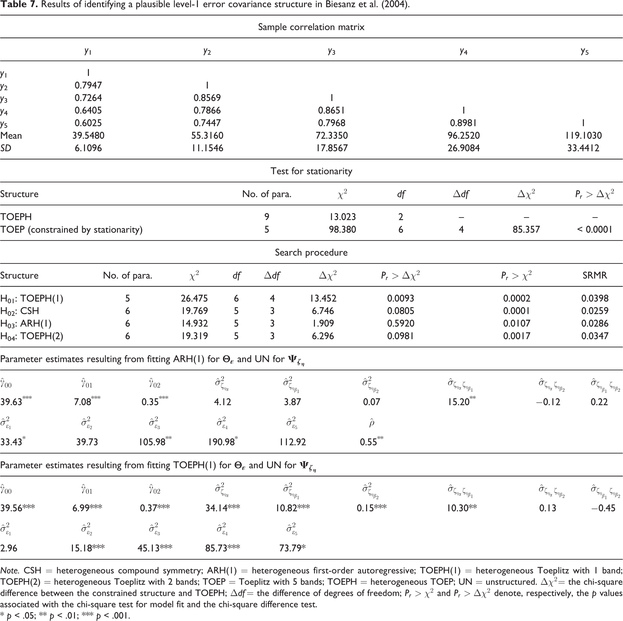
Note. CSH = heterogeneous compound symmetry; ARH(1) = heterogeneous first-order autoregressive; TOEPH(1) = heterogeneous Toeplitz with 1 band; TOEPH(2) = heterogeneous Toeplitz with 2 bands; TOEP = Toeplitz with 5 bands; TOEPH = heterogeneous TOEP; UN = unstructured. $Δ χ_{}^{2}$ = the chi-square difference between the constrained structure and TOEPH; Δdf= the difference of degrees of freedom; $P_{r} > χ_{}^{2}$ and $P_{r} > Δ χ_{}^{2}$ denote, respectively, the p values associated with the chi-square test for model fit and the chi-square difference test.

* p < .05; ** p < .01; *** p < .001.

Discussion

As mentioned previously, the impact of the misspecification of the level-1 error covariance structure could be substantial. In this study, we have, under the principle of achieving both model fit and parsimony, proposed a systematic approach, based on the chi-square difference test, to facilitate identifying a plausible covariance structure. Preliminary simulation results have shown the usefulness of the proposed approach. The rate of correct identification is an increasing function of sample size. Moreover, we have verified that acceptable parameter estimates result from the correct covariance structure only.

Computational convergence problems may occur during the process of estimation. To handle the problems, researchers need to provide appropriate initial values for the parameters to be estimated (Li, Duncan, Duncan, & Acock, 2001). In our simulation studies, we used their population values as initial values to facilitate estimation, as frequently seen in the literature (e.g., Chen, 2007). In practice, however, population parameter values are unknown. SAS PROC CALIS determines initial values by using a combination of such methods as two-stage least squares estimation, instrumental variable method, approximate factor analysis method, ordinary least squares estimation, estimation method of McDonald, and observed moments of manifest exogenous variables (SAS Institute Inc., 2014). Although they perform reasonably well in most common applications, there is no guarantee of convergence. If non-convergence occurs during the search procedure, we suggest that the parameter estimates resulting from fitting a structure that has achieved convergence be used as initial values and rerun. To further reduce the chance of encountering estimation problems, we suggest using larger series lengths (larger than the minimum T required, shown in Table 2) and larger sample sizes.

When the covariance structure is less constrained, the estimates of variances/covariances are more likely to be linearly related. Although their linear relationships do not affect the model fit and the effectiveness of the chi-square difference test, if the structure identified by the proposed approach contains linearly related parameter estimates, restrictions need to be imposed to obtain unique solutions.

Although our demonstrations were based on unconditional linear and quadratic growth models, the approach is applicable for more general situations such as polynomial level-1 submodels with time-varying predictors, conditional LGM, with time-invariant predictors in level-2 submodels, and the second-order LGM (for investigating the trajectory of a construct over time) (e.g., Bollen & Curran, 2006, Ch. 8; Hancock, Kuo, & Lawrence, 2001). For non-linear growth functions (non-linear in the parameters), non-linear transformations of either time or the repeated measures could be used, and then the usual linear model is fitted to transformed outcome (e.g., Bollen & Curran, 2006, Sec. 4.4).

There exist some limitations of the proposed approach. First, the growth function needs to be well determined (by substantive theory) before searching for a suitable error covariance structure. When a growth model is misspecified, parameter estimates converge to different values from those of a correctly specified model, and the chi-square difference test can be misleading (Yuan & Bentler, 2004). When the theoretical support for a growth function is absent, Kim, Kwok, Yoon, Willson, and Lai (2016) gave a strategy to search for a correct polynomial growth model. They showed that the starting model with the saturated level-1 error covariance structure (UN) resulted in higher rates of correct identification than that with the simplest covariance structure, i.e., TOEP(1). Moreover, the chi-square difference test performs well in searching for the optimal mean trajectory. Once the true mean structure has been identified, the true level-1 error covariance structure can be subsequently determined by using the proposed approach, completing the two-step approach mentioned by Kim et al. (2016). Second, the data are assumed to be equally spaced in time in order to test stationarity, because, for unequally spaced data, some autocovariances at lag k, k ≥ 1 are unestimable. One way to deal with unequally spaced data is to interpolate the data to even spacing before conducting the stationarity test, assuming that the growth function has been well determined. Third, larger samples are needed to attain a required rate of correct identification for smaller numbers of time points and/or lower autocorrelations. Fourth, since there may be many model comparisons in the proposed approach, the Type-1 error rate of rejecting a specific covariance structure when it is true may be much inflated. Fifth, a plausible level-1 error covariance structure is selected from those shown in Table 1. If the true structure is not nested within the least constrained structure, the procedure will miss the true structure. Including more covariance structures and developing a more comprehensive identification approach deserve future research.

Footnotes

Acknowledgments

The authors thank Dr. Todd D. Little, the Methods and Measures Editor, and three anonymous reviewers for their constructive comments and suggestions, which greatly improved the quality of the paper.

Funding

The author(s) declared receipt of the following financial support for the research, authorship, and/or publication of this article: This research was partially supported by grants NSC98-2410-H-009-010-MY2 and NSC100-2410-H-009-008-MY2 from the Ministry of Science and Technology, R.O.C.

References

Anderson

J. C.

Gerbing

D. W.

(1988). Structural equation modeling in practice: A review and recommended two-step approach. Psychological Bulletin, 103, 411–423.

Biesanz

J. C.

Deeb-Sossa

Papadakis

A. A.

Bollen

K. A.

Curran

P. J.

(2004). The role of coding time in estimating and interpreting growth curve models. Psychological Methods, 9, 30–52.

Bollen

K. A.

Curran

P. J.

(2006). Latent curve models: A structural equation perspective. Hoboken, NJ: Wiley & Sons.

Box

G. E. P.

Jenkins

G. M.

Reinsel

G. C.

(1994). Time series analysis: Forecasting and control (3rd ed.). Englewood Cliffs, NJ: Prentice-Hall.

Chen

F. F.

(2007). Sensitivity of goodness of fit indexes to lack of measurement invariance. Structural Equation Modeling, 14, 464–504.

de la Torre

van der Ark

L. A.

Rossi

(2015). Analysis of clinical data from cognitive diagnosis modeling framework. Measurement and Evaluation in Counseling and Development. Advance online publication. doi:10.1177/0748175615569110

Ding

C. G.

Jane

T. D.

(2012). Using SAS PROC CALIS to fit level-1 error covariance structures of latent growth models. Behavior Research Methods, 44, 765–787.

Ferron

Dailey

(2002). Effects of misspecifying the first-level error structure in two-level models of change. Multivariate Behavioral Research, 37, 379–403.

Hancock

G. R.

Kuo

W. L.

Lawrence

F. R.

(2001). An illustration of second-order latent growth models. Structural Equation Modeling, 8, 470–489.

10.

Hoogland

J. J.

Boomsma

(1998). Robustness studies in covariance structure modeling: An overview and a meta analysis. Sociological Methods & Research, 26, 329–367.

11.

Kim

Kwok

O. M.

Yoon

Willson

Lai

M. H. C.

(2016). Specification search for identifying the correct mean trajectory in polynomial latent growth models. Journal of Experimental Education, 84, 307–329.

12.

Kwok

O. M.

West

S. G.

Green

S. B.

(2007). The impact of misspecifying the within-subject covariance structure in multiwave longitudinal multilevel models: A Monte Carlo study. Multivariate Behavioral Research, 42, 557–592.

13.

Duncan

T. E.

Duncan

S. C.

Acock

(2001). Latent growth modeling of longitudinal data: A finite growth mixture modeling approach. Structural Equation Modeling, 8, 493–530.

14.

Murphy

D. L.

Pituch

K. A.

(2009). The performance of multilevel growth curve models under an autoregressive moving average process. Journal of Experimental Education, 77, 255–282.

15.

SAS Institute Inc. (2014). SAS/STAT 9.4 user’s guide. Cary, NC: SAS Institute Inc.

16.

Sivo

Fan

(2008). The latent curve ARMA (p,q) panel model: Longitudinal data analysis in educational research and evaluation. Educational Research and Evaluation, 14, 363–376.

17.

Widaman

K. F.

Thompson

J. S.

(2003). On specifying the null model for incremental fit indices in structural equation modeling. Psychological Methods, 8, 16–37.

18.

Wolfinger

(1996). Heterogeneous variance: Covariance structures for repeated measures. Journal of Agricultural, Biological, and Environmental Statistics, 1, 205–230.

19.

West

S. G.

Taylor

A. B.

(2009). Evaluating model fit for growth curve models: Integration of fit indices from SEM and MLM frameworks. Psychological Methods, 14, 183–201.

20.

Yuan

Bentler

P. M.

(2004). On the chi-square difference and z tests in mean and covariance structure analysis when the base model is misspecified. Educational and Psychological Measurement, 64, 737–757.