Multi Small Index (MSI): A spatial indexing structure

Abstract

Most of the existing spatial indices are constructed using a single hierarchal index structure; hence a large number of index pages (nodes) are most likely to be inspected during spatial query execution. Since spatial queries usually fetch spatial objects based on their spatial position in the space, it is significant that spatial objects are clustered in such a way that pertinent objects to a query are fetched quickly. This paper presents a method for partitioning the whole space into set of small subspaces. Then, an index structure for each subspace (called the Multi Small Index) is built. This makes it is easy to quickly retrieve spatial objects that are relevant to the query in question using their corresponding small spatial index structures and ignoring other irrelevant indices. To evaluate our new approach, we conducted a set of experimental studies using a collection of real-life spatial datasets (TIGER data files) with diverse sizes and different object sizes, densities and distributions, as well as various query sizes. The results show that (using small query sizes) our proposed structure (Multi Small Index) outperforms the original R-tree (Single Big Index) structure, achieving nearly 50% saving in disk access.

Keywords

R-tree space partitioning spatial database spatial index spatial queries

1. Introduction

Spatial data are important in many application areas, such as geographical information systems and computer-aided design. Spatial database systems manage large collections of spatial data that is stored based on its spatial attributes. A commonly used query on spatial data is to search for all objects that overlap a spatial area; this is denoted as range (or region query). This kind of spatial search occurs frequently, and therefore it is important to be able to retrieve spatial objects efficiently. To do this, spatial indices are used to organize spatial objects in a way that will enable an efficient retrieval of query relevant objects according to their spatial attributes.

To meet the needs of spatial indexing, numerous spatial access methods (e.g. R-tree [1], R⁺-tree [2], R^*-tree [3], SR-tree [4], SB⁺-tree [5] (extension of the B⁺-tree [6]), Packed R-tree [7] and X-tree [8]) have been proposed. Usually, spatial indices are designed in such a way such that each node fits in one page in the disk [9]. When a spatial query is executed, an algorithm is used to access the disk and navigate the index to retrieve relevant objects. The performance of a spatial data structure is usually evaluated by the ability to answer range queries by accessing the smallest possible number of pages in the disk [10]. A challenging research problem is to improve the efficiency of spatial queries by reducing number of disk accesses used.

The problem is that, when a single spatial index is built for all data objects in a space, the entire index is searched to retrieve relevant objects. For a region query to be answered, the query region is spatially located in the space and the objects overlap that region must be retrieved. However, since all objects in the space are inserted in a single index, this index includes: (1) those objects that overlap the query region (relevant objects); (2) objects spatially adjacent to the query region but not overlapping it (possibly relevant); and (3) those objects that are spatially distant from the query region (irrelevant). The purpose of this paper is to determine the effect of grouping the spatial objects on the number of disk accesses needed to answer a certain region query.

It is important to group spatial objects in a manner that relevant spatial objects to a query are retrieved quickly. This can be done by merging the objects into groups in a smart way, where groups with possibly relevant objects can be distinguished quickly from groups without such objects. Thus, the key issue for spatial objects is to find useful groupings of such objects.

Spatial data structures must be made efficient in terms of storage space, time required to insert or delete objects, and time required to query responses. Usually, it is difficult to improve efficiency in terms of both storage and time. Generally, faster queries require greater storage and more pre-processing and updating time [11].

On designing a spatial index, several challenging issues regarding objects in the spatial space, such as overlapping [12] and splitting [13], have received much of researchers’ attention. In contrast, the main idea in this paper is to pay attention to the spatial space itself, which we introduced in a previous paper [14] and substantially extend here, where it has been described in more detail and evaluated experimentally.

Single Big Index (SBI) refers to the single index built for all objects in a spatial space S, which is the traditional approach for constructing spatial indices. As we mentioned above, in answering a spatial query Q using SBI structure, you will retrieve objects that are relevant, possibly relevant and irrelevant to Q. This slows down the search operation. In this paper, we propose a new approach for partitioning the space into groups, such that relevant and possibly relevant objects are stored in a group different from that of irrelevant objects. This means that the query navigates directly relevant groups and skips checking irrelevant objects. An efficient way to group spatial objects is to partition spatial space. By partitioning a spatial space S into a set of small subspaces, each subspace will have its own smaller indexing structure. Consequently, we will have a set of small index structures, referred to as a Multi Small Index (MSI).

To build an MSI structure for a set of spatial object covered by space S, S is partitioned into smaller subspaces in different level such that (1) each resulting subspace has its length and width equal to half the length and width of the space from which it directly came, and (2) the resulting final subspaces have capacities that are slightly different. We called the proposed partitioning procedure Dynamic Recursive Quartiles (DRQ) partitioning. Each partitioning step of DQR creates four equal subspaces (quartiles). After each partitioning step, each resulting subspace is recursively partitioned until the partitioning threshold value is met. This threshold value is set to ensure a reasonable performance for the MSI structure. The resulting subspaces are called target spaces (TSs). After that, an index structure is created for each target space.

The remainder of this paper is organized as follows. Section 2 presents an overview of related spatial index structures. We present our new approach MSI structure in Section 3. Section 4 presents the experimental evaluation. In Section 5, we summarize our paper and discuss possible future research directions.

2. Related work

The goal of spatial access methods is to organize spatial data to enable efficient retrieval of relevant objects according to the topological properties of their spatial attributes. Spatial data is characterized by its complex structure; it may be composed of a single point or several thousands of polygons with arbitrary distribution and no order in the space. Usually, a spatial query (e.g. a region or point query) requires fast execution of a search operation that retrieves data objects based on their locations in the space. To efficiently perform such search operations, it is important to develop an efficient index structures for spatial data.

To efficiently handle different shapes of spatial objects (e.g. point, line, circle), there should some kind of a generic geometric shape approximation to interface with spatial index structures and hence to reduce the number of false hits, as well as computation time. The most commonly used spatial shape approximation is the minimum bounding rectangle (MBR). It is utilized in many spatial index structures such as R-tree [1], R⁺-tree [2] and R^*-tree [3]. Other shape approximations exist, such as minimum bounding spheres (MBS) in the sphere tree [15], and the balltree [16]; the intersection of an MBS with MBR in SRtree [4]; hyper-rectangles of arbitrary orientation [17]; a convex hull [18]; and polyhedra [19].

In the literature, various spatial index structures are proposed to efficiently access spatial data. The majority of these access methods are based on a space partitioning scheme. The main idea is to partition the data space into smaller sub-regions using the divide and conquer concept. Each partition operation produces an inner node in the index structure. This process continues until each partition contains a number of spatial objects that fit a page (node) capacity. Each leaf node of the index structure contains addresses of spatial objects that are contained in the corresponding sub-region.

Some of the existing spatial access methods use regions to structure special objects into groups. The main idea behind these methods is to represent spatial objects using rectangles, spheres or others shape approximations. The regions may overlap (such as R-tree [1]) or pair-wise disjoint (such as R⁺-tree [2]). Many proposed indexing techniques are based on R-tree. R⁺-tree [2], R^*-tree [3], X-tree [8], Hilbert R-tree [20] and Linear R-Tree [21] are examples of R-tree-based indexing methods.

The index structures must be able to organize not only points, but also any geometrical shape. To be indexed, many spatial indices reduce the geometrical shapes of the objects to rectangles that are referred to as the MBRs.¹ For a spatial object, the MBR is the smallest axes-parallel rectangle that fully encloses the geometry of the spatial object [22]. Other indices use a sphere to reduce the geometrical shape of the objects. R-tree is a dynamic index structure in which spatial objects can be inserted on a one-by-one basis and they do not need to be known before tree construction. On the other hand, other R-tree variants require that all objects are known prior to the tree construction; these versions of R-tree are called static index structures.

The R-tree is one of the most popular data structures to index spatial objects that have spatial extent (e.g. lines and rectangles). It is an extension of the B-tree [23] to index multidimensional data space.

There are two types of R-tree nodes: leaf nodes and non-leaf nodes. Each leaf node contains entries of the form (rect, oid) where oid is a pointer refers to a particular spatial object bounded by the MBR rect. Each non-leaf node contains entries of the form (rect, ptr), where ptr is the address of a child node and rect is the MBR that spatially covers all rectangles in the child node’s entries. To guarantee at least 50% storage utilization, every node in R-tree, except the root, must have at least m and at most M entries, where m ≤ ⌊M/2⌋ and M is the node capacity. The root node can have at least two children nodes unless it is a leaf where it can have one object. An R-tree for a data space of size N has the maximum height ⌊log_m N⌋ − 1.

Searching the R-tree is done by looking for all nodes whose MBRs intersect a query window. The search operation starts with the root locating all child nodes whose MBRs overlap the search window, then recursively searches the subtrees of those child nodes until a leaf node is reached. Then it tests all entries in the leaf node and returns all leaf entries that overlap the query window.

Since the MBRs of spatial objects stored in the index structure are allowed to overlap, searching may require traversing several tree paths. The larger MBRs coverage area leads to the larger probability of MBR intersecting the query window. This may lead to visiting many paths and nodes during the search operation and, to minimize that, the area of the MBRs should be minimized. To enhance the search operation, there should be an efficient way to dynamically distribute MBRs of spatial objects in such a way that minimizes the number of tree paths visited during a spatial query.

Inserting an object in the R-tree index means adding new entry in one of the leaf nodes; nodes that overflow are split and the generated changes propagate up the tree. The first operation in the object insertion is to find a leaf in which the new entry is to be inserted. The leaf selection will start from the root and will follow the path denoted by the entries whose MBRs need least enlargement in order to contain the MBR of the new object. Thus, at each level, the least enlarged node is chosen. Finally, if there is a space available, the object is inserted in the leaf; otherwise the node must be split into two nodes. Node splitting leads to minimizing the sum of the areas of the two resulting nodes. Several node splitting algorithms exist in the literature [24 –26].

3. Proposed approach

In this section, we present our structure that we called MSI and present the method proposed for space partitioning to construct the MSI. We called the space partitioning method DRQ partitioning. A well-computed threshold value is used to direct the DRQ partitioning. MSI relies on the R-tree spatial index; therefore we will present our findings using R-trees.

When a spatial space that contains single huge group of objects is partitioned into a collection of subspaces, this will create multiple groups of these objects and then virtually distant objects are separated in different target spaces and at the same time objects adjacent to each other are grouped into similar target spaces. For N objects that belong to a global space S, we partition S into multiple subspaces, such that each part of N will belong to a different subspace. For each resulting subspace a relatively small index structure is created. This collection of the resulting small-index structures is referred to as the MSI structure.

3.1. Dynamic Recursive Quartiles partitioning

In this DRQ partitioning method, spaces are partitioned continuously until a criterion is met; each time a partitioning operation is performed on the space, four subspaces are produced, and we call them quartiles. The DRQ partitioning method is performed using the following procedure. Initially, a threshold is computed to drive all the partitioning operations. After that, for each space, global space or subspace, we check whether its capacity is greater than the computed threshold; if so, we partition the space into four new quartiles, Otherwise, it is not partitioned. We refer to those subspaces that need no further partitioning because their capacities are less than or equal to the threshold as target spaces, because they are the final subspaces for which a collection of R-tree indices will be constructed.

We can demonstrate partitioning procedure as levels. Initially, the global space is partitioned into four subspaces called the first-level quartiles. If any of the first-level quartiles are partitioned, then four quartiles in the second level are produced under the partitioned quartile and so on. Generally, for any quartile in the ith level that is partitioned, four new quartiles in the (i + 1)th level are produced in the lower level. We build a tree for the quartiles in each level such that each tree node contains four quartiles. Let S be the global space and let us refer to the four quartiles at the left-bottom, right-bottom, left-top, and right-top as S0, S1, S2 and S3, respectively. Then, for a partitioning operation on any subspace Sx, the four resulting quartiles will be named as Sx0, Sx1, Sx2 and Sx3 for the left-bottom, right-bottom, left-top, and right-top, respectively. Finally, any space Sx with capacity not greater than the threshold is a target space. Figure 1 depicts space naming clearly and the resulting quartiles tree.

Figure 1.

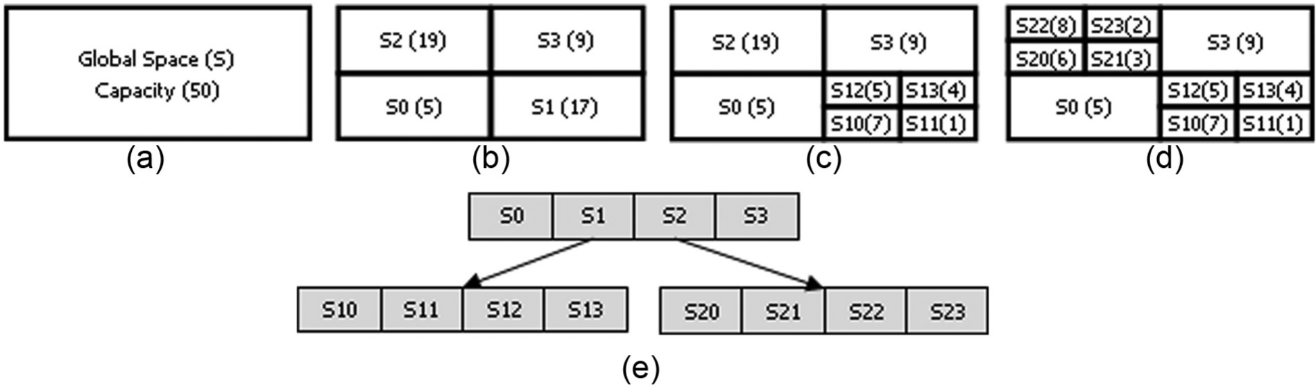
Process of DRQ partitioning method, threshold = 10. (a) Global space with capacity = 50; (b) first partition operation; (c) second operation; (d) third operation; and (e) the quartiles tree.

Target spaces are the smallest subspaces resulting from DRQ partitioning and an R-tree index will be constructed for all of them to contain all of the objects of the global space. To access the target spaces of the partitioned space, we build a tree to store the coordinates of each target space as a metadata; we refer to this tree as the metaTree. Internal nodes of the metaTree belong to partitioned spaces and are composed of four items to store the coordinates of the four quartiles resulting from this partitioning. In addition to the coordinates of the quartile, each item in the internal nodes contains a pointer to a child node in the lower level. In leaf nodes of the metaTree, each of the four items contains the coordinates of its corresponding target space in addition to a pointer to the R-trees built to store all the objects overlapping with this target space.

In Figure 1, a space S with capacity of 50 is to be partitioned using DRQ partitioning with a threshold value of 10 objects. First, the global space S is partitioned since its capacity is greater than 10 and four quartiles resulting with names S0, S1, S2 and S3. A node for these four quartiles is created in the first level as shown in Figure 1(e). Then each space is checked to determine whether it needs further partitioning in the order left-bottom, right-bottom, left-top and right-top. Both S0 and S3 need no partitioning. S1 and S2 have to be partitioned because their capacity is greater than the threshold. Partitioning S1 generates four new quartiles, S10, S11, S12 and S13, with capacities of seven, one, five and four, respectively, each of which is now a target space because its capacity is not greater than 10, as shown in Figure 1 (c). A node for these four quartiles is created in the second level under S1, as shown in Figure 1 (e). The same process is performed on S2. Its capacity is 19 and it is partitioned to produce S20, S21, S22 and S23. All of them do not need further partitioning and they are now target spaces, as shown in Figure 1 (d). A node for these four quartiles is created in the second level under S2, as shown in Figure 1 (e). Note that three partitioning operations are performed and the number of target spaces is 10.

For description issues in this paper, for a specific partitioned space, let us refer to the group of the target spaces as the target spaces group (TSG). Only the subspaces whose capacity is less than or equal to the threshold are members of the TSG. Target spaces represent the contents of leaf nodes. Let us refer to the number partitioning operations performed to partition a space as p, and let us refer to the total number of target spaces by t, which is the size of TSG. We can derive the following formula: t = 4 × p − p + 1 = 3 × p + 1.

The formula is derived as follows. Gavin a space S to be partitioned, assume arbitrarily that S is a member in TSG. Therefore, initially t = 1. Each partition operation produces four new subspaces that will be inserted into the TSG. At the same time, the partitioned space itself is removed from the TSG and replaced by its new quartiles. In other words, each partition operation triggers four insertions and one removal operation on TSG. For a total of p operations, the number of insertions will be 4 × p and the number of removals will be p. Therefore, the t value will be 4 × p − p plus the initial space. Figure 1(d) shows that three partition operations produce 3 × 3 + 1 = 10 target spaces. The distribution of objects affects how the global space is partitioned and which subspace is partitioned. For example, the space in Figure 1(d) has more objects in the left-top region than the left-bottom region.

3.2. Threshold used

The threshold used to perform DRQ space partitioning affects space partitioning significantly in terms of:

The size of TSG, t. The larger the threshold value the smaller the number of target spaces.

Target space capacity. The larger the threshold value the larger the capacity of target spaces in TSG.

Number of objects overlapped multiple target spaces. A small threshold value allows more partitioning operations to be performed, which creates more dividing lines across the space. Consequently, the number of objects that touch the dividing lines will probably increase and this will increase the number of objects sharing multiple spaces. The smaller the threshold value, the larger will be the numberof objects sharing multiple target spaces.

Therefore, choosing a suitable threshold value is very important since it has an effect on the space partitioning and the indexing performance.

3.3. Definition of MSI

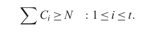
Given a spatial space S with capacity N and with TSG = {TS₁, TS₂, TS₃, …, TS_t} organized in the metaTree, an MSI structure is a set of t indices ranging from R₁ to R_t built to index the N objects of S, such that each index R_i in MSI represents an access method for c_i objects that overlap a corresponding target space TS_i in TSG. Since objects may overlap multiple target spaces and then they will be inserted in more than one index in MSI, it must be noted that

\sum C_{i} \geq N : 1 \leq i \leq t .

3.4. MSI construction

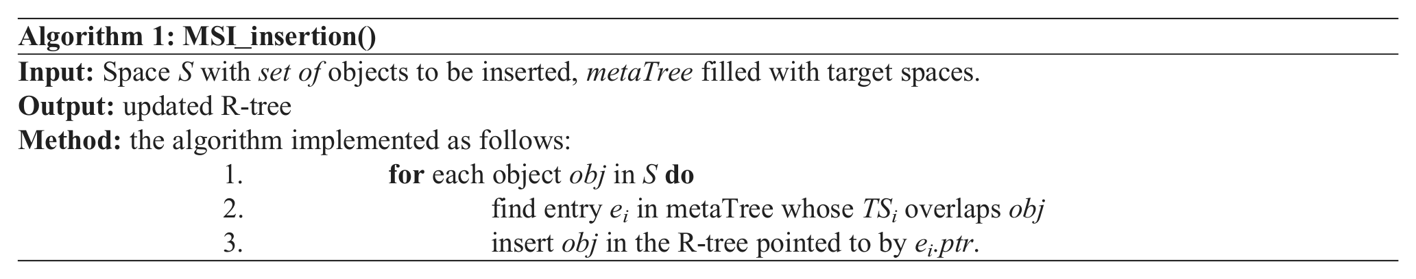
For each object obj, we find overlapping target space TS_i in the metaTree and insert obj in the R-tree index pointed to by the entry in which the TS_i is stored. The way by which insertion is performed in MSI is described in Algorithm 1.

3.5. Searching in MSI structure

One of the general types of queries is to find all objects overlapping a query region. Let Q refer to an instance of a query of this type. Searching in MSI is performed by finding each TS_i that overlaps Q. If Q overlaps multiple target spaces, say r, then we partition Q to r sub-regions (SQs). Each SQ represents the region of intersection between Q and each overlapping target space. Then, we continue by executing each SQ intersecting TS_i over the corresponding R-tree in MSI structure. Algorithm 2 describes the way in which searching is performed in MSI. A sample of a query region and how it is partitioned into two SQs is shown Figure 2.

Figure 2.

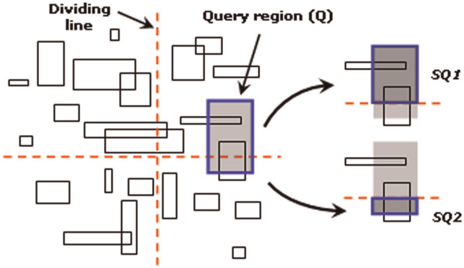
Sample target spaces to show the partitioning of a query region Q to two sub-queries SQ₁ and SQ₂.

A spatial space with capacity of 28 objects and two query regions Q₁ and Q₂ is shown in Figure 3. Seven target spaces resulted from the partitioned process using the DRQ partitioning method. Both SBI and MSI structures are built for this same space, as shown in Figures 4 and 5. In Figure 3, Q₁ and Q₂ overlap S₂₀ and S₃, respectively. To answer the query of Q₁ using SBI structure, search procedure must traverse the R-tree index shown in Figure 4, which may be expensive compared with using MSI, where the search procedure will traverse the metaTree to access the R-tree of S20 shown in Figure 5 and retrieve relevant objects. To answer the query of Q₂ using SBI, the search procedure must navigate the R-tree index shown in Figure 4, whereas using MSI, search procedure must navigate the metaTree to access the R-tree of S3 shown in Figure 5 and retrieve relevant objects.

Figure 3.

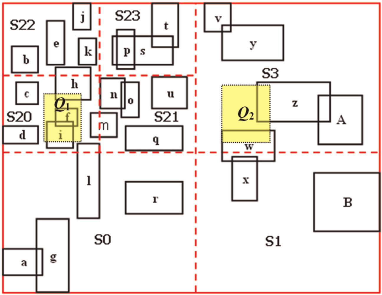
Space partitioned using DRQ partitioning method.

Figure 4.

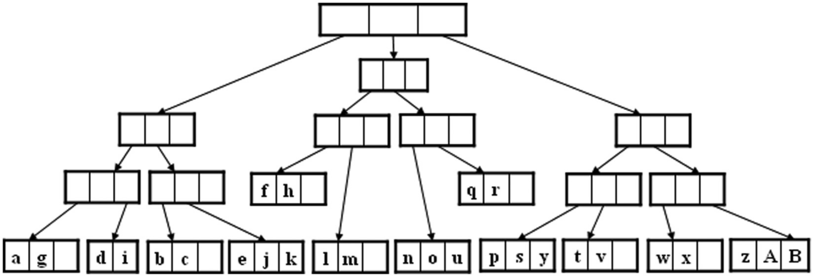
R-tree SBI structure created for the space in Figure 3.

Figure 5.

R-tree MSI structure for the space in Figure 3.

3.6. MSI advantages

Compared with SBI, MSI represents a collection of indices each with smaller height than that of SBI. In the worst case, the height of any index in MSI will be less than or equal to that of SBI. This is because, for a space with capacity N, there is no way for an index in MSI to include more than N objects. A key point in MSI is that, once we want to execute a region query, we will navigate relatively small indices with small height compared with the SBI with the large height. To retrieve objects that overlap a given region Q, in our indexing method, we just navigate the index of the (possibly) relevant objects to Q, which is the index of each target space that overlaps Q, and skip others. That is, we constrain the search operation to look for an answer in objects spatially adjacent (relevant) to Q and leave those objects that are spatially distant from (irrelevant to) Q.

The small indices of MIS introduce just the relevant objects to be searched for a specific query and enable the query to skip those irrelevant objects. In SBI all objects in the space are inserted in one index, so the index includes relevant and irrelevant objects to a specific query region. Hence, the region query may check unnecessary nodes, which may increase the cost of answering the query. Searching just the necessary objects enforces better search performance during index navigating, instead of searching relevant and irrelevant objects that may burden the search performance.

It must be noted that the metaTree created to organize the target spaces does not burden the search performance since it is a single unit in its entirety and it has small size, so it fits in memory. Accessing the metaTree does not require any disk access during the search performance. Each partition operation for the space triggers the creation of a metaTree node. Each metaTree node occupies 20 bytes to store the four coordinates of a rectangle and a pointer for the child node in each of the four entries. For a total of 100 partitioning operations, that is, p = 100, we have 100 tree nodes. Therefore, we have 100 × 20 = 2000 bytes to store the metaTree, which is small enough and can be stored in the main memory.

4. Experimental evaluation

In this section, we present a description of the region queries usually used for the evaluation of the performance of a spatial data structure in Section 4.1. In Section 4.2, we describe performance factors that affect the work performance of spatial indexing. Datasets and types of the data objects used for our experiments are depicted in Section 4.3. We illustrate each dataset and the place from which it is extracted, and the type of the objects in each. In Section 4.4, we explain the threshold used for our DRQ partitioning method and how it is derived. In Section 4.5, we describe the experimental setup for our query region search. We describe the size and the location of query regions that are used in our experiments. The experimental results are described in Section 4.6. In Section 4.7 construction issues of MSI are described, such as number of target spaces, number of shared objects and number of splitting operations performed during its construction.

In our experiments, we partition various spaces using DRQ partitioning method described in Section 3, and then we build an MSI using the target spaces resulted from the partitioning. We perform our experiments with three aims:

to determine whether the MSI built for a space meets an acceptable performance level when answering a region query compared with the SBI structure;

to test the performance of MSI under different spaces;

to evaluate the performance of MSI using various region queries with different locations and sizes.

4.1. Region queries

One method for the evaluation of the performance of a spatial data structure is the ability to answer a range query, specified by a query region, by accessing the smallest possible number of pages in the disk [27]. Other queries, such as nearest neighbour queries [28] or topological queries (e.g. meet, covers) [29], are useful but not representative of the efficiency of a spatial data structure. As a result, all of the efforts to evaluate the performance of spatial data structures, particularly R-trees, have focused on range query [10]. In our experiments, the region query is the only query type used. The region query looks up the spatial objects that intersect a given region window. In a two-dimensional space, two points need to be provided for a region query: the left-bottom corner point and the right-top point.

4.2. Performance factors

When using the R-tree, the cost of region queries [30], in terms of number of disk accesses, is affected by many factors. The height of the R-tree influences the search performance because it is an indication of the number of tree nodes that have to be tested during the search path. When the tree height increases, this may increase the number of disk accesses required to answer a query. Another thing that influences the search operation is the location of the query region. Different locations of a query region may lead to different search paths through the R-tree, which may influence the number of disk accesses required to answer the query. The length and width of the query region also influence the cost of the search in a high degree. The length and width of a query region indicates its size. They influence the number of candidates selected by the filter step. The larger the query size, the greater the number of candidates is, and the more expensive the query. Using the SBI index structure to answer a region query requires navigation through the same index, visiting probably different search paths. For static data, the SBI index has a fixed height. However, in the case of MSI, the same region query may use an R-tree with height less that of SBI. To study this case experimentally, different query regions with different locations and sizes are used to make sure various R-trees in the MSI structure are accessed.

4.3. Datasets

To ensure the generality of our experimental results, real spatial datasets (TIGER/Line data files [31]) are used with different properties. The TIGER data is developed and distributed by the US Bureau of the Census, and contains detailed cartographic information for the USA [32]. Different types of TIGER/Line data objects are used, such as area objects representing districts, roads, river segments, railroads, shore lines and streams. Each TIGER data object is represented by four coordinates representing the object’s MBR. We used the following types of data objects:

Areas – areas and tract boundaries inside the counties represent sections in different parts of the USA. For our experiments, we computed the MBRs of all the areas and used them as spatial data. We refer to this type of data object as ‘Tareas’.

Roads and railroad – objects from TIGER that give the road data as line segments; long roads are divided into short segments. For our experiments, we computed the MBRs of all of the roads and railroads and used them as spatial data. We refer to this type of data object as ‘Troads’.

River segments and shore lines – objects composed of rivers that include large and small streams of water and shore lines (lines on the beach where the water meets the sand). Also, for our experiments, we computed the MBRs of all the river segments and shore lines and used them as spatial data. We refer to this type of data object as ‘Trivers’.

Mix of objects of type Troads and Trivers. We refer to this type of data object as ‘Tmix’.

Table 1 shows the spatial data used in our experiments, which is a collation of 19 spatial datasets containing objects of different types, sizes, and places in the USA.

Table 1.

Datasets used in experiments.

State	Counties	Type	Size	Name
Pennsylvania	York, Adams and Franklin	Roads	52,729	PA_ro
		Rivers	11,045	PA_ri
		Areas	16,963	PA_a
		Mix	63,775	PA_m
California	Los Angeles	Roads	85,657	Los_ro
		Rivers	6,101	Los_ri
		Areas	95,043	Los_a
		Mix	191,759	Los_m
Texas	20 counties	Roads	199,133	TX_ro
		Rivers	23,486	TX_ri
		Areas	64,703	TX_a
Nevada	All counties	Roads	320,143	NV_ro
		Rivers	54,629	NV_ri
		Areas	64,837	NV_a
		Mix	374,772	NV_m
Alabama	All counties	Roads	598,311	AL_ro
		Rivers	120,943	AL_ri
		Areas	138,572	AL_a
		Mix	714,453	AL_m

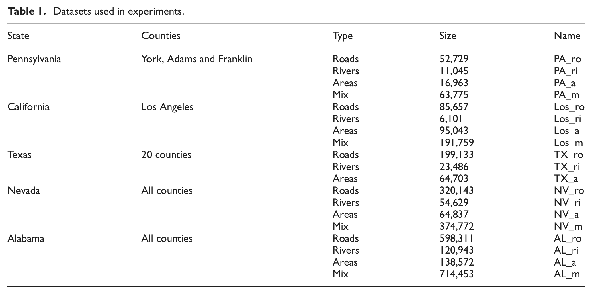
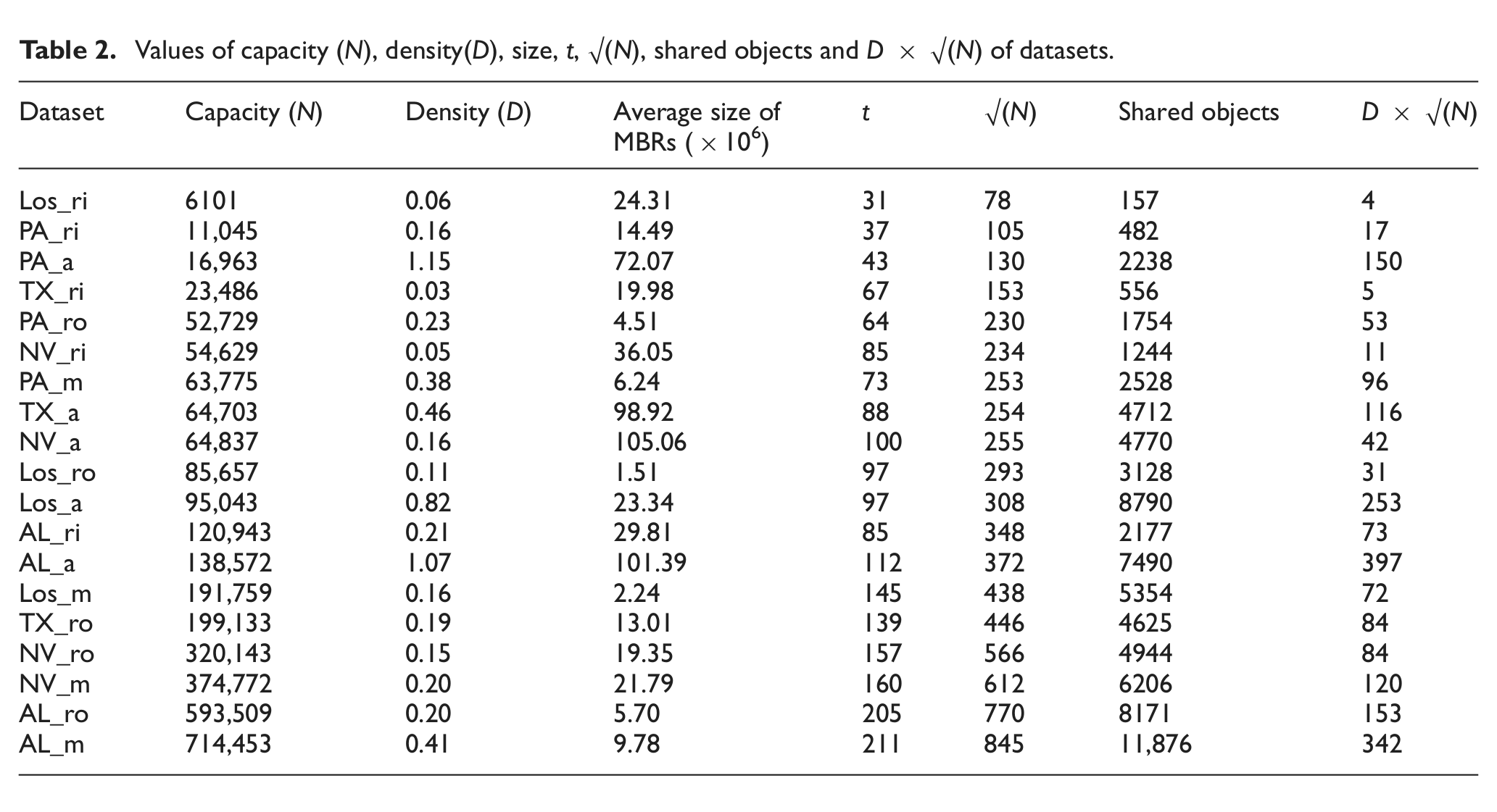
Note that the data objects are collected from various places in the USA. One collection contains data for eastern US states (Pennsylvania), others for western US states (California, Nevada) and further ones for southern US states (Texas, Alabama). Datasets represent spaces with different capacities, densities and sizes. Table 2 shows this difference. Object density is the total area of the rectangles divided by the area of the workspace [33, 34]. Object density will have an effect on the performance of the spatial index. An increase in object density may increase the number of objects that overlap a given search area. More tree nodes will require navigation, and then the cost of the search will increase. The size is represented by the average size of all data objects in the space. Estimating the distribution of the objects inside spaces is the most difficult factor. In many cases the object distribution is not known, and even if it is known, its properties are very hard to capture [35]. Our data objects contain objects from different distributions.

Table 2.

Values of capacity (N), density(D), size, t, √(N), shared objects and D × √(N) of datasets.

Dataset	Capacity (N)	Density (D)	Average size of MBRs (×10⁶)	t	√(N)	Shared objects	D × √(N)
Los_ri	6101	0.06	24.31	31	78	157	4
PA_ri	11,045	0.16	14.49	37	105	482	17
PA_a	16,963	1.15	72.07	43	130	2238	150
TX_ri	23,486	0.03	19.98	67	153	556	5
PA_ro	52,729	0.23	4.51	64	230	1754	53
NV_ri	54,629	0.05	36.05	85	234	1244	11
PA_m	63,775	0.38	6.24	73	253	2528	96
TX_a	64,703	0.46	98.92	88	254	4712	116
NV_a	64,837	0.16	105.06	100	255	4770	42
Los_ro	85,657	0.11	1.51	97	293	3128	31
Los_a	95,043	0.82	23.34	97	308	8790	253
AL_ri	120,943	0.21	29.81	85	348	2177	73
AL_a	138,572	1.07	101.39	112	372	7490	397
Los_m	191,759	0.16	2.24	145	438	5354	72
TX_ro	199,133	0.19	13.01	139	446	4625	84
NV_ro	320,143	0.15	19.35	157	566	4944	84
NV_m	374,772	0.20	21.79	160	612	6206	120
AL_ro	593,509	0.20	5.70	205	770	8171	153
AL_m	714,453	0.41	9.78	211	845	11,876	342

4.4. Threshold value

As described in Section 3.3, space partitioning is performed using a partitioning threshold. Since the main purpose of partitioning the space is to create the MSI structure, the threshold used in this partitioning significantly affects the MSI structure in the following ways:

Total number of trees in MSI – the smaller the threshold value is, the larger the number of trees in the MSI.

The number of objects indexed by each tree in MSI, which is the number of objects overlapping the corresponding target space – the smaller the threshold value is, the smaller the number of objects inserted in each MSI tree.

Height of each tree in the MSI – the smaller the threshold value is, the smaller the height of each MSI tree.

Number of objects indexed in multiple trees in the MSI – objects that overlap multiple target spaces must be inserted in multiple trees in the MSI. The smaller the threshold value is, the greater the number of objects shared in multiple trees in MSI.

In general, for any space S, let h refers to the threshold value used for partitioning S and let h_b refers to the best threshold value that causes the best performance of the MSI of S. Also, let h_p and h_t refer to the number of partitioning operations and the size of TSG resulting from using h_b, respectively. Finally, let n refer to the number of objects that overlap multiple target spaces. In our experiments we reported the following observations about threshold value:

Using a threshold value <h_b forces the number of performed partitioning operations to be >h_p, that is, the size of TSG t is >h_t. Also, this will cause the number of objects that overlap multiple spaces to be >n.

Using a threshold value >h_b forces the number of performed partitioning operations to be <h_p, that is, the size of TSG t is <h_t. Also, this will cause the number of objects that overlap multiple spaces to be <n.

Both of the above cases cause the MSI performance to be worse than the best performance. In the first case (h < h _b), the number of indexing trees will increase owing to the increase in t and this will increase the probability of a query region overlapping multiple target spaces and being executed over multiple trees, which will increase number of disk accesses necessary to answer a query region. In the second case (h > h_b), the number of indexing trees will decrease owing to the decrease in t. Although this will decrease the probability of a query region overlapping multiple target spaces, when this occurs, the search will be executed over the MSI trees with heights greater than the height of the trees that resulted when using h_b as a threshold, which will increase the number of disk accesses necessary to answer a query region.

Using a fixed threshold does not work for all spaces. This is because spaces have different capacities, and a threshold that causes good performance in one space may not cause good performance in spaces with larger or smaller capacity. To obtain the suitable partitioning threshold we performed the following steps:

For each dataset (described in the previous section), we tried different thresholds values ranging from 1 to 50% of the space capacity. Then we created an MSI structure for the partitioned spaces.

For each space partitioned using a specific threshold value, we executed various region queries (as described below) of different sizes and locations in the space and report the average number of disk accesses needed to answer the queries.

For the same spaces, we created an SBI on which we executed the same region queries.

For each space, we compared the performance of the MSI against the SBI using every tested partitioning threshold and report the best threshold on which MSI gets the best performance.

By following the above steps, we determined the best threshold for each space by which the space is to be partitioned and an MSI structure with a good performance was created. We noted that all of the values of the best thresholds were always <10% of the space capacity. After that we determined a formula to obtain a number close to the threshold value for each space relying on the properties of that space. Space properties that can be used to derive such formula are: (1) the capacity of the space; (2) the work space area, which is the area of the minimum bounding rectangle that covers all the space objects; (3) the size of objects in the space; (4) the density of objects in the space; and (5) object distribution in the space, which is very difficult to capture [35].

The density of objects combines both the work space area and the size of objects in the space; therefore, we adapted the density to represent both. Object density can be computed using the formula:

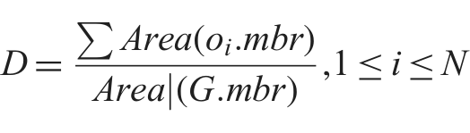
D = \frac{\sum Area (o_{i} . mbr)}{Area | (G . mbr)}, 1 \leq i \leq N

where D denotes the density, o_i.mbr is the MBR of object o_i, and G.mbr denotes the MBR of the global space. The derived formula for the threshold must give a value that falls between 1 and 10% of the space. Also, we have to take into consideration the number of objects that intersect the dividing lines, that is, number of shared objects between multiple subspaces.

The partitioning procedure stops space partitioning only when each subspace contains a number of objects smaller than or equal to the threshold. Unfortunately, there are extra partitioning operations caused by the effect of shared objects. Shared objects arbitrarily participate in the decision of partitioning subspaces. For example, let the capacity of a space S to be 190 and suppose two subspaces A and B, subspace A having 100 objects and B having 90 objects. With a partitioning threshold of 95, only subspace A has to be partitioned. On the other hand, suppose, for the same space, that there are 10 shared objects between A and B causing the capacities of A and B to be, for example, 103 and 97, respectively. In this case, both A and B will be partitioned since their capacities are >95. In this case, the shared objects invoked the partitioning procedure to partition both A and B. This problem can be solved by increasing the threshold. For example, if we increase the threshold value in the last case by 5, then space A will be partitioned and space B will be not. Therefore, the effect of the shared objects is alleviated by allowing the threshold value to take the shared objects into consideration.

For a dividing line l in a partitioned space, the number of objects that overlap l (number of shared objects) is affected by number of dividing lines and the object density. When we partitioned the above spaces, it was found that √(N) is an indication of the number of target spaces t (√(x) is the square root of x). √(N) gives a value that is almost four times greater than t. Table 2 shows the number of target spaces (t) for our dataset and the value of √(N). Since each subspace is bounded by four lines, they all affect the number of objects shared between this subspace and adjacent ones. Therefore, we used √(N), instead of √(N)/4, to indicate the number of dividing lines in the space.

In spatial spaces, the line chart that represents the number of shared objects in some partitioned space can be represented by the formula D × √(N). Table 2 contains the number of shared objects resulting from partitioning the spaces described in the previous section, and the values of D × √(N) for the same spaces. It is clear that they have the same behaviour when a line chart is drown for each of them. Therefore, D × √(N) should be a reasonable parameter to compute the threshold value.

Because DRQ partitioning produces four subspaces each time we partition a space, log₄N should be a reasonable parameter for computing the threshold value. log₄N represents how deeply the space is partitioned, that is, the height of the metaTree that organizes the subspaces resulting from space partitioning. As we mentioned above, for our datasets, we found that the best partitioning threshold should be <10% of the space capacity. To obtain a value that is always <10%, the formula log₄N × √(N) always gives a value that is <10% of the space capacity. Therefore, we used the formula log₄ N × √(N) + D × √(N) to form a threshold by which we partitioned the spaces, which was experimentally tested. All results shown in the next sections are based on this formula.

4.5. Experimental setup

To test the influence of a range query size and location on the performance of the indexing structure, we divided each dimension of the data space into 1000 units. Different square query sizes were used ranging from square side 5 to 200 of the data space. For each query size, 1000 region queries were randomly generated. The number of disk accesses utilized by each of 1000 queries was recorded. We used these numbers to compute the average and the maximum number of disk accesses per query. We did not compute the time needed to answer the region queries since, as mentioned in Arge et al. [36], disk access is a stronger measure of performance, and the query time is easily affected by operating system caching and by disk page layout. Another reason is that research on spatial databases and its indexing is heavy computer work where not much cache memory is available or where caches are ineffective. Therefore, we can say that disk access dominates the query time.

4.6. Experimental results

In this section, we describe the experiments that we performed to discover the performance of MSI and then present the results of the experiments. To perform experimental comparison between MSI and SBI structures, the R-tree was used to construct both structures. We refer to the average number of disk accesses of the MSI and SBI as DA(MSI) and DA(SBI), respectively. Saving in disk access of MSI is denoted by

1 - \frac{D A (M S I)}{D A (S B I)} \times 100 %

Also, we refer to the maximum number of disk accesses needed by MSI and SBI as maxDA(MSI) and maxDA(SBI), respectively. Here, we use SBI as a measuring standard for the MSI, that is, we standardize maxDA(SBI) to 100% such that we can observe the performance of the MSI relative to the 100% performance of the SBI. The relative improvement in terms of maximum disk access of the MSI is denoted by

\frac{\max D A (M S I)}{\max D A (S B I)} \times 100 %

The average number of disk accesses is a stronger measurement than the maximum number of disk accesses. Therefore, taking the maximum number of disk accesses as a measurement is not clear enough. Therefore, we will describe this using an example. Table 3 shows the results of executing three query regions Q₁, Q₂ and Q₃ on both SBI and MSI structures. The number of disk accesses for each query is reported. Then, the average and the maximum are computed. There exist four cases for the results as shown in Table 3. In the Structure row of Table 3, the name of the structure that gives the better performance is in bold. Also, in the Average and Maximum rows, the smaller values are in bold.

Table 3.

Sample of different cases for three region queries showing the average and maximum number of disk accesses needed by the MSI and SBI structures.

	Case 1		Case 2		Case 3		Case 4
	SBI	MSI	SBI	MSI	SBI	MSI	SBI	MSI
DA(Q ₁)	2	4	6	4	6	3	5	7
DA(Q₂)	3	4	1	4	4	2	5	1
DA(Q₃)	3	4	1	4	4	2	4	1
Average	2.7	4.0	2.7	4.0	4.7	2.3	4.7	3.0
Maximum	3	4	6	4	6	3	5	7

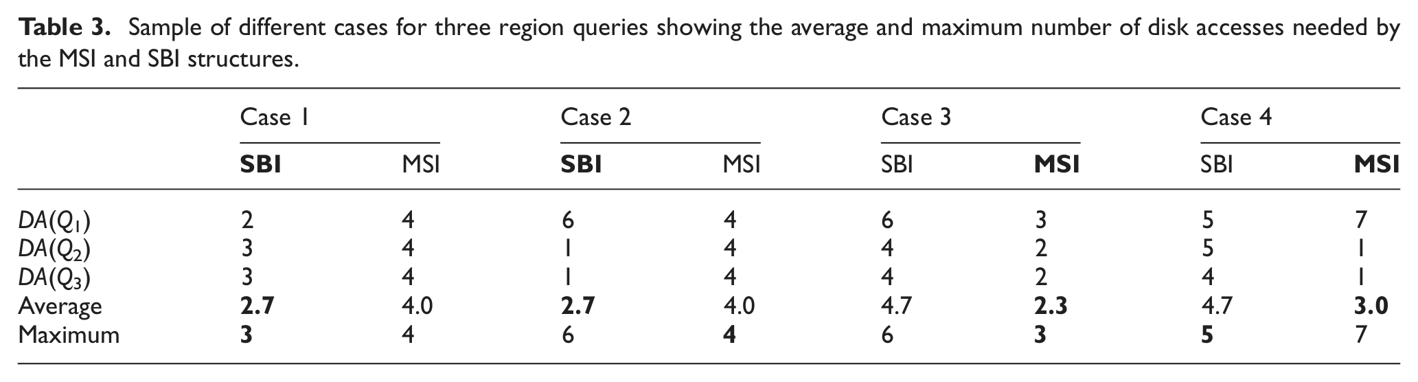
In case 1, SBI is better; this indicated by both the average and the maximum disk accesses.

In case 2, SBI is also better; this is indicated by the average. However, note that the maximum number of disk accesses for MSI is smaller than that for SBI, which is a good indicator of the benefit of MSI. Even though the average disk access for SBI is smaller, we can guarantee that the maximum number of disk accesses needed by any query region using MSI structure is smaller than that of SBI.

In case 3, MSI is better; this indicated by both the average and the maximum disk accesses. Also, in this case, the maximum number of disk accesses is an indicator for the benefit of MSI, so that we guarantee that the maximum number of disk accesses needed by any query region using MSI structure is smaller that that of SBI.

In case 4, MSI is better; this indicated by the average number of disk accesses.

Since the height of any tree in the MSI must be less or equal to the height of SBI, the case where the maximum number disk access needed by MSI is larger than SBI is unlikely to happen. If it does happen, this will be for a query that navigates multiple trees in MSI.

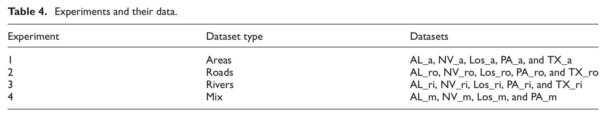
In our experiments, to create the MSI structure, we partitioned the space using different threshold values and report the value of the best threshold h_b that causes the best performance. Therefore, we show the results of the MSI using h_b.The experiments performed are described in Table 4.

Table 4.

Experiments and their data.

Experiment	Dataset type	Datasets
1	Areas	AL_a, NV_a, Los_a, PA_a, and TX_a
2	Roads	AL_ro, NV_ro, Los_ro, PA_ro, and TX_ro
3	Rivers	AL_ri, NV_ri, Los_ri, PA_ri, and TX_ri
4	Mix	AL_m, NV_m, Los_m, and PA_m

Figures 6 –9 show the disk access saving achieved by MSI using the datasets of types Tareas, Troads, Trivers and Tmix, respectively. The relative maximum number of disk accesses utilized by MSI using datasets of types Tareas, Troads, Trivers and Tmix are shown in Figures 10 –13, respectively.

Figure 6.

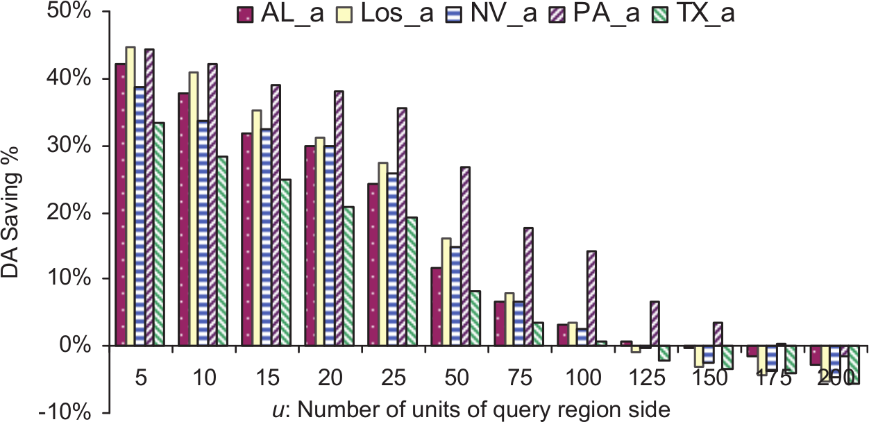
Saving in disk access achieved using MSI on datasets of type Tareas.

Figure 7.

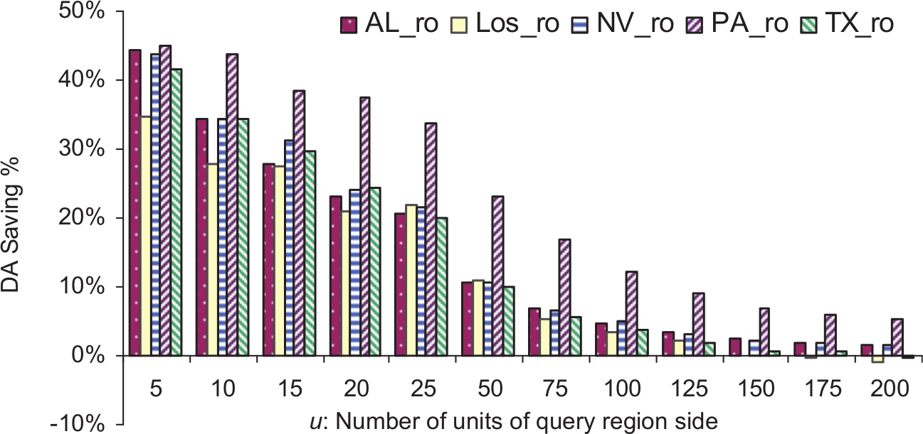
Saving in disk access achieved using MSI on datasets of type Troads.

Figure 8.

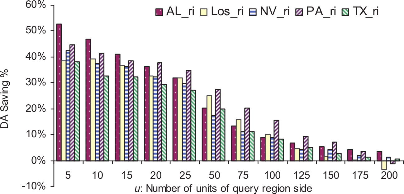
Saving in disk access achieved using MSI on datasets of type Trivers.

Figure 9.

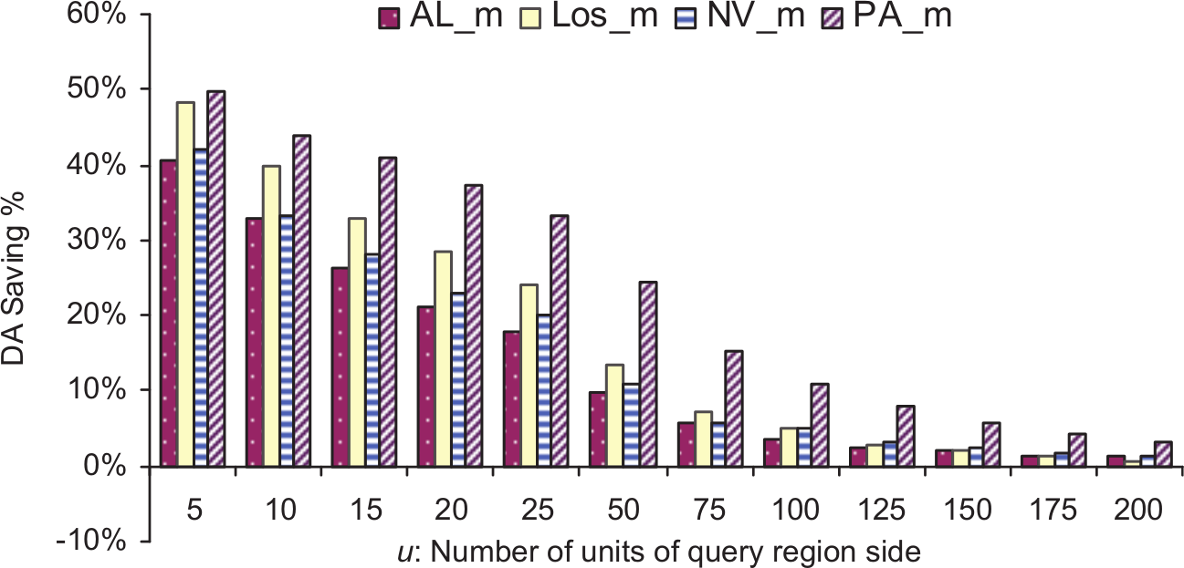
Saving in disk access achieved using MSI on datasets of type Tmix.

Figure 10.

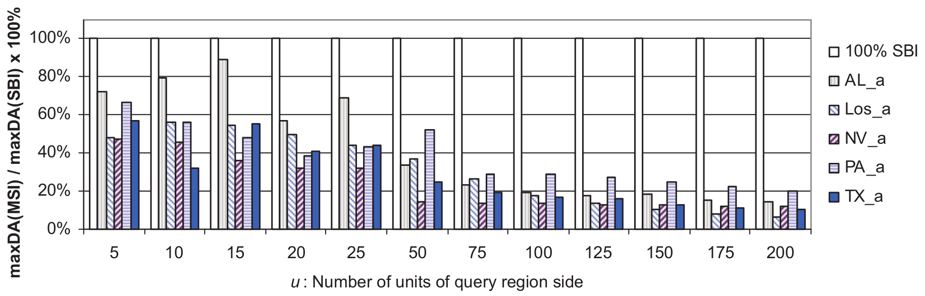
Maximum number of disk accesses needed by MSI relative to 100% of SBI on objects of type Tareas computed as maxDA(MSI)/maxDA(SBI).

Figure 11.

Maximum number of disk accesses needed by MSI relative to 100% of SBI on objects of type Troads computed as maxDA(MSI)/maxDA(SBI).

Figure 12.

Maximum number of disk accesses needed by MSI relative to 100% of SBI on objects of type Trivers computed as maxDA(MSI)/maxDA(SBI).

Figure 13.

Maximum number of disk accesses needed by MSI relative to 100% of SBI on objects of Tmix type computed as maxDA(MSI)/maxDA(SBI).

4.7. Results analysis

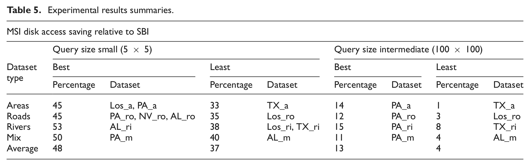
In Figures 6 –13, it can be seen that MSI structure performs better for small query regions because these tend to overlap just one target space and navigate just one index. In the case of large query region, it is more likely to overlap multiple target spaces and then search more than one tree in MSI. For example, using datasets of type Tareas, the best disk access saving was achieved using both Los_a and PA_a datasets, which is almost 45% of the small region query size. On the other hand, the least disk access saving for small query regions was 33% using TX_a data set. For query regions larger than 100 × 100, SBI outperformed MSI. The maximum number of disk accesses needed per query using MSI was always lower than that for the SBI structure. The same scenario occurred for the other three dataset types (roads, rivers and mix). Also, we noticed that MSI always outperformed SBI for small and large region query sizes using datasets of the types Troads, Trivers and Tmix, and this was true using datasets of type areas for region queries of sizes less than 100 × 100. We summarize all of the experimental results in Table 5.

Table 5.

Experimental results summaries.

MSI disk access saving relative to SBI
Dataset type	Query size small (5 × 5)				Query size intermediate (100 × 100)
	Best		Least		Best		Least
	Percentage	Dataset	Percentage	Dataset	Percentage	Dataset	Percentage	Dataset
Areas	45	Los_a, PA_a	33	TX_a	14	PA_a	1	TX_a
Roads	45	PA_ro, NV_ro, AL_ro	35	Los_ro	12	PA_ro	3	Los_ro
Rivers	53	AL_ri	38	Los_ri, TX_ri	15	PA_ri	8	TX_ri
Mix	50	PA_m	40	AL_m	11	PA_m	4	AL_m
Average	48		37		13		4

5. Conclusions and future work

Spatial queries are supported by spatial datasets, where these queries must achieve fast access to sought data based on its space location. However, a common method, SBI, is used to index a whole dataset space. Since spatial queries retrieve objects relevant to their location, spatial objects need to be indexed such that relevant objects to a query are retrieved quickly, while irrelevant objects are ignored. In this paper, a new efficient index structure, MSI, is presented. The main idea is to partition the spatial space into subspaces using a new partitioning method, DRQ; afterwards, the subspaces are structured as a metadata tree to access a collection of R-trees; one R-tree is created for each subspace.

The MSI structure was evaluated and compared against the SBI structure experimentally, using real datasets of different object types (roads, areas, and rivers) and different capacity. The dataset objects differed in their density, distribution, and size. A set of spatial queries was used to evaluate the performance of the proposed index structure. They had different sizes and were distributed randomly over the space. Our experimental results show that MSI outperformed the SBI structure in the number of disk accesses used to answer a range query. However, the performance of the MSI structure depended considerably on the query size. The results show that, for small query sizes, the MSI structure may achieve a 50% saving in disk access. Also, MSI always outperformed SBI for small and large region query sizes used for datasets of types roads, rivers and mix, and this was true using datasets of type areas for region queries of sizes not greater than 100 × 100.

For future work, the MSI structure will be applied using other R-tree variants such as R^*-tree and R⁺-tree. Moreover, parallelism can be applied during the execution of the MSI structure, such that each index is managed independently, and if a query region overlaps multiple spaces, a method can be used to allow sub-queries to be executed in parallel to obtain better results.

Footnotes

Acknowledgements

The authors would like to express their deep gratitude to the anonymous referees for their helpful comments and suggestions which improved the paper.

Notes

References

Guttman

. R-Trees: A dynamic index structure for spatial searching. In: Proceedings of the ACM SIGMOD international conference on management of data. New York: ACM Press, 1984.

Sellis

Roussopoulos

Faloutsos

. The R+-Tree: A dynamic index for multi-dimensional objects. In: Proceedings of the 13th conference on very large databases. Brighton: (Morgan Kaufmann, 1987.

Bechmann

Kriegel

Schneider

Seeger

. The R*-tree: An efficient and robust access method for points and rectangles. In: Proceedings of the ACM SIGMOD international conference on management of data. Atlantic City, NJ: ACM Press, 1990).

Katayama

Satoh

. The SR-tree: An index structure for high dimensional nearest neighbor queries. Proceedings of the international conference on management of data, 1997; 360–389.

Ibrahim

Fotouhi

Al-Badarneh

. Efficient processing of spatial selection and join operations using SB+-tree. In: Proceedings of international database engineering and applications symposium. Montreal: IEEE Computer Society, 1997.

Knuth

. The art of computer programming: Sorting and searching, 2nd edn. Reading, MA: Addison-Wesley, 1967.

Poussopoulos

Leifker

. Direct spatial search on pictorial databases using packed R-tree. In: Proceedings of the ACM SIGMOD international conference on management of data. Austin, TX: ACM Press, 1985.

Berchtold

Keim

Kriegel

. The X-tree: An index structure for high-dimensional data. In: Proceedings of the 22th conference on very large databases. San Francisco, CA: Morgan Kaufmann, 1996.

Tomás

Jaroslav

Václav

. PM-tree: Pivoting metric tree for similarity search in multimedia databases. In: Proceedings on the ADBIS conference, 2004.

10.

Theodoridis

Sellis

. A model for the prediction of R-tree performance. In: Proceedings of the 15th ACM SIGACT-SIGMOD-SIGART symposium on principles of database systems. New York: ACM Press, 1996.

11.

Haverkort

. Results on geometric networks and data structures. PhD thesis, Utrecht University, 2004.

12.

Tao

Papadias

Zhang

. Cost models for overlapping and multi-version structures. ACM Transactions on Databases Systems 2002; 27(3): 299–342.

13.

Brakatsoulas

Pfoser

Theodoridis

. Revisiting R-tree construction principles. In: Proceedings of the 6th ADBIS conference. London: Springer, 2002.

14.

Al-Badarneh

Al-Alaj

. A spatial index structure using dynamic recursive space partitioning. In: Proceedings of international conference on innovations in information technology, 2011.

15.

Philip

. Collision detection for interactive graphics applications. IEEE Transactions on Visualization and Computer Graphics 1995; 1(3): 218–230.

16.

Omohundro

. Five balltree construction algorithms. Technical report TR-89-063, International Computer Science Institute, 1989. Available at: http://ftp.icsi.berkeley.edu/ftp/pub/techreports/1989/tr-89-063.pdf (accessed 14 December 2012).

17.

Gottschalk

Lin

Manocha

. Obb-tree: A hierarchical structure for rapid interference detection. In: Proceedings of the 23rd annual conference on computer graphics and interactive techniques. New York: ACM Press, 1996.

18.

Brinkhoff

Kriegel

Schneider

Seeger

. Multi-step processing of spatial joins. In: Proceedings of the 1994 ACM SIGMOD international conference on management of data. New York: ACM Press, 1994.

19.

Jagadish

. Spatial search with polyhedra. In: Proceedings of the sixth international conference on data engineering. Montreal: IEEE Computer Society, 1990.

20.

Kamel

Faloutsos

. Hilbert R-tree: An improved R-tree using fractals. In: Proceedings of the 20th international conference on very large data bases. San Francisco, CA: Morgan Kaufmann, 1994.

21.

Al-Badarneh

Tawil

. Linear R-tree revisited. International Journal of Computers and Applications 2009; 31(2): 74–83.

22.

Clementini

Sharma

Egenhofer

. Modeling topological spatial relations: Strategies for query processing. Computer and Graphics 1994; 18: 815–822.

23.

Comer

. The ubiquitous B-tree. ACM Computing Surveys 1979; 11(2): 121–137.

24.

Liu

Fang

Han

. A new R-tree node splitting algorithm using MBR partition policy. In: Proceedings of the 17th international conference on geoinformatics, 2009.

25.

Al-Badarneh

Yaseen

Hmeidi

. A new enhancement to the R-tree node splitting. Journal of Information Science 2010; 36(1): 3–18.

26.

Korotkov

. A new double sorting-based node splitting algorithm for R-tree. Programming and Computer Software 2012; 38(3): 109–118.

27.

Brakatsoulas

Pfoser

Theodoridis

. Revisiting R-tree construction principles. In: Proceedings of the 6th East European conference on advances in databases and information systems. London: Springer, 2002.

28.

Song

Park

Kong

K-S

Lee

. Bottom-up nearest neighbor search for R-trees. Information Processing Letters 2007; 101(2):78–85.

29.

Papadias

Theodoridis

Sellis

Egenhofer

. Topological relations in the world of minimum bounding rectangles: A study with R-trees. In: Proceedings of the 1995 ACM SIGMOD international conference on management of data. New York: ACM Press, 1995.

30.

Corral

Manolopoulos

Theodoridis

Vassilakopoulos

. Cost models for distance joins queries using R-trees. Data Knowledge Engineering 2006; 57(1): 1–36.

31.

US Bureau of Census, TIGER/Line files, Washington, DC. Available at: http://www.census.gov/geo/www/tiger/rd_2ktiger/tgr2kweb.html (accessed 14 December 2012).

32.

Patel

DeWitt

. Partition based spatial-merge join. In: Proceeding of the 1996 ACM SIGMOD international conference on management of data. New York: ACM Press, 1996.

33.

Papadias

Mamoulis

Theodoridis

. Processing and optimization of multiway spatial joins using R-trees. In: Proceedings of the eighteenth ACM SIGMOD-SIGACT-SIGART symposium on principles of database systems. New York: ACM Press, 1999.

34.

Manolopoulos

Nanopoulos

Papadopoulos

Theodoridis

. R-Trees have grown everywhere (unpublished manuscript). Available at: http://delab.csd.auth.gr/papers/TRSurveyRtree03_mnpt.pdf (accessed 15 December 2012).

35.

Mamoulis

Papadias

. Multiway spatial joins. ACM Transactions on Database Systems 2001; 26(4): 424–475.

36.

Arge

Berg

Haverkort

. The priority R-tree: A practically efficient and worst-case-optimal R-tree. ACM Transactions on Algorithms 2008; 4(1): 9:1–9:30.