LDA topics: Representation and evaluation

Abstract

In recent years many automated topic coherence formulas (using the top-m words of a topic inferred by latent Dirichlet allocation) based on word similarities have been proposed and evaluated against human ratings. We treat a wordy topic as an object and quantitatively describe it via normalized mean values of pair-wise word similarities. Two types of word similarities, thesaurus and local corpus-based, are used as the descriptive features of a topic. We perform topic classification using represented topics as input and bi-level human ratings about topic coherence as class labels. Classification results (precision, recall and accuracy) based on two datasets and three supervised classification algorithms suggest that the novel topic representation is consistent with human ratings. Corpus-based word similarities are positively correlated with human ratings whereas thesaurus-based similarities have negative relations. The proposed representation of topics opens a window for us to investigate the utilization of topics with different perspectives.

Keywords

Latent Dirichlet allocation (LDA)supervised classification topic model topic representation topic evaluation topic coherence

1. Introduction

Topic models learn thematic topics from words that tend to co-occur in a collection of documents. Each inferred topic is a collection of words over a fixed vocabulary and the words in a topic are sorted based on the probability values of word occurrences in it. Topics can be used to explain and retrieve documents and this explanation (of a document) is only useful if we can understand what is meant by a given topic. To evaluate topics, researchers [1 –7] usually use top-m words and employ humans to collect an interpretability score. Once m (for top-m words of a topic) is picked, it is fixed for each topic in a particular experiment. In recent years, task-independent strategies for evaluating topic models have been developed. Newman et al. [1], Mimno et al. [2], Aletras and Stevenson [3], Rosner et al. [4] and Röder et al. [5] proposed topic coherence formulas and showed that these measures correlated with human judgment. Lau et al. [6] evaluated topic coherence and topic model quality and also automated the task of finding top words in a topic. Chang et al. [7] used human judgment to evaluate the quality of topic models, presented quantitative methods for measuring semantic meaning in topics and showed that their methods capture aspects of the model that are undetected by previous measures of model quality based on held-out likelihood.

The majority of automatic coherence formulas [1 –3, 6] are based on a single-word similarity measure. Amongst the similarity measures the point-wise mutual information (PMI) [1, 6] and its variations [6] are found to be best matched with human ratings. Coherence measures [4, 5] were adopted from psychology theory and showed better topic interpretability compared with other measures [1, 2]. Human judgments about topic meaning/interpretation are found to conflict with each other [5] and they are expensive to collect in real time. Hinneburg et al. [8] pointed out that the most probable top words of a topic may leave room for ambiguous interpretation, especially when the top words are exclusively nouns. They claimed more interpretable topic representations from the use of part-of-speech tagging and co-location analysis of terms to derive linguistic frames [8].

Our proposition is that, if interpretability of top-m words of a topic is not agreed upon by humans and there is no single agreed coherence formula, then why not change the way we use top-m words. Use of top-m words is included in almost every coherence measure, but there is no single attempt to replace wordy representation of topics by quantitative representation. Our question was, can we represent a topic in a quantitative way, and then use it in place of a wordy topic? To answer this question we treated each topic as an object and then looked for its descriptive characteristics/features. We used mean values of word similarity features to represent a topic (top-m words) in a quantitative way (see equations 1–9). More concrete ways to analyse this novel thinking was helped through the use of topic-coherence scores judged by human annotators. We presented wordy topics to human annotators and got their binary level feedback in terms of topic-coherence scores (see Table 2 for some examples of topics). In our definition, a topic is good if humans can identify its title; otherwise it is bad (see Section 3.4). Next, we used quantitative representation of topics (Table 3) to train supervised classification algorithms to assess whether the proposed features represent the topics faithfully or not.

2. Related work

In recent years, for a set of words (or topics), different word similarities have been used in automated coherence formulas [1 –3, 6] and in finding the best words [6] from this collection of words. Newman et al. [1] proposed many topic (top-10 words) coherence measures based on two types of word similarities: WordNet and Wikipedia corpus. A topic was assumed to be coherent if it had a higher average pair-wise similarity between words. One of their coherence formulas is well known as UCI where a similarity feature is PMI, and it provided the largest correlations with human ratings. We used six WordNet similarities (Section 3.3.1) in common with Newman et al. [1] and the seventh feature in common is PMI (Section 3.3.2). The difference is the domain type and the size of the corpora. We used smaller corpora that belong to the news domain whereas they used Wikipedia articles; we used average similarities as descriptive features of a topic and they treated them as separate coherence formulas. Mimno et al. [2] introduced an asymmetrical coherence formula (UMass) by replacing the PMI of UCI with conditional probability, based on the local corpus used to generate the topics. The summation of UMass coherence accounts for the ordering among the top-m (M = 5, 10, 15, 20) most probable words of a topic. We also experimented with UMass and used it as a descriptive feature in our experiments (not reported in our results), but it was not improving the accuracy of our classifiers and showed less correlation with human ratings (see Tables 7 and 8).

Aletras and Stevenson [3] proposed coherence formulas based on distributional similarity features using the top-10 words of a topic. Each topic word was represented as a vector (weighted by PMI or normalized PMI) in a semantic space (using a window of size $\pm 5$ over a Wikipedia corpus) [3], consisting of information about word co-occurrence. Topic coherence was determined by measuring the distance between word vectors using a similarity metric. Three of our corpus-based features (Cosine, Jaccard and Dice; see Section 3.3.2) are in common with Aletras and Stevenson [3]. The difference is that we use term frequency inverse document frequency (TF-IDF) weightings rather than PMI weightings. Lau et al. [6] found systematic differences between intruder words and observed coherence of a topic, and improved the state of the art for automatic evaluation of observed coherence. They also utilized PMI and its variations to find word similarities and they aggregate the topic coherence score into a single-topic model-level score.

3. Materials and methods

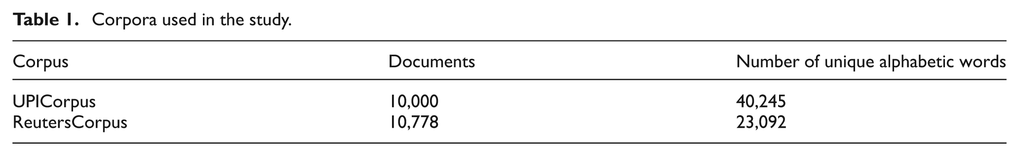
The materials used are two corpora (Table 1), inferred topics (Table 2) and the datasets (Table 3). The methods are preprocessing (Section 3.1), extracting topics using latent Dirichlet allocation (LDA) (Section 3.2), word similarity measures and topic representation (Section 3.3), topic annotations (Section 3.4) and preparation of datasets (Section 3.5.1) to train classifiers (sections 3.5.2–3.5.4). Major steps in our proposed methodology (Figure 1) are discussed in this section, with the aim being to explain the necessary information related to our experiments, the algorithms used and their specific parameter settings, so that results will be reproducible. Equations (1)–(9), are about the proposed topic representation scheme and are listed in Sections 3.2 and 3.3.

Table 1.

Corpora used in the study.

Corpus	Documents	Number of unique alphabetic words
UPICorpus	10,000	40,245
ReutersCorpus	10,778	23,092

Table 2.

Examples of Good and Bad topics with mean coherence and topic labels.

No.	Topic	mCoh	Label
1	add Monday hold end start recent follow rally gain meanwhile	0.428571	Bad
2	air aircraft space station flight launch land fly mission plan	1	Good
3	area mile damage report official local resident hour region warn	0.571429	Bad
4	attack kill bomb violence target suspect carry claim link attempt	0.857143	Good

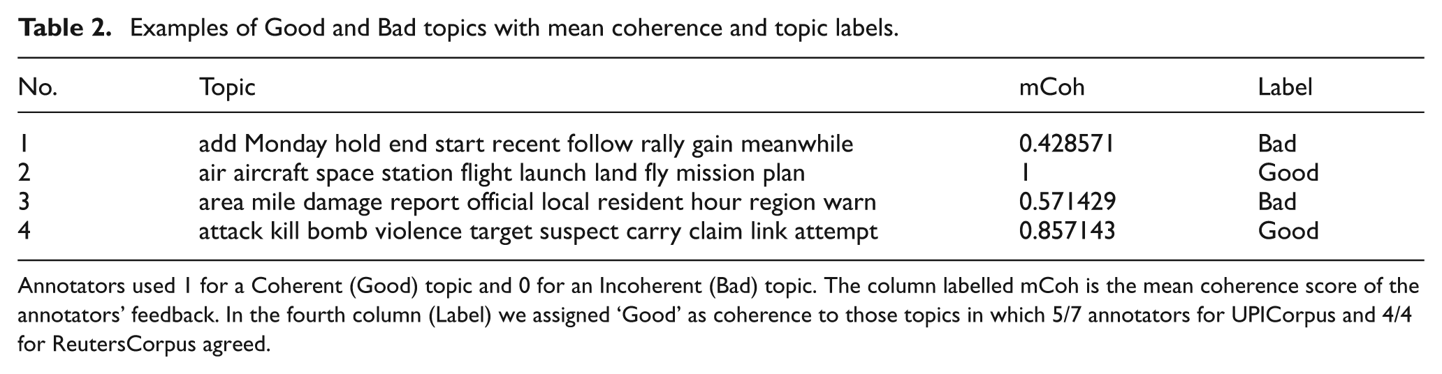
Annotators used 1 for a Coherent (Good) topic and 0 for an Incoherent (Bad) topic. The column labelled mCoh is the mean coherence score of the annotators’ feedback. In the fourth column (Label) we assigned ‘Good’ as coherence to those topics in which 5/7 annotators for UPICorpus and 4/4 for ReutersCorpus agreed.

Table 3.

Some examples of represented topics and their associated labels.

No.	nCos	nJac	nDice	nPmi	nPath	nLch	nWup	nRes	nJcn	nLin	Coh
1	−0.49	−0.06	−0.11	−0.42	0.24	0.08	0.23	−0.04	0.04	−0.04	Bad
2	−0.09	−0.01	−0.02	0.66	−0.11	0.08	−0.10	0.06	0.04	0.05	Good
3	0.11	−0.00	0.00	−0.08	−0.27	−0.10	−0.27	−0.12	−0.03	−0.11	Bad
4	−0.41	−0.05	−0.08	0.05	−0.09	−0.03	−0.09	0.02	−0.06	0.02	Good

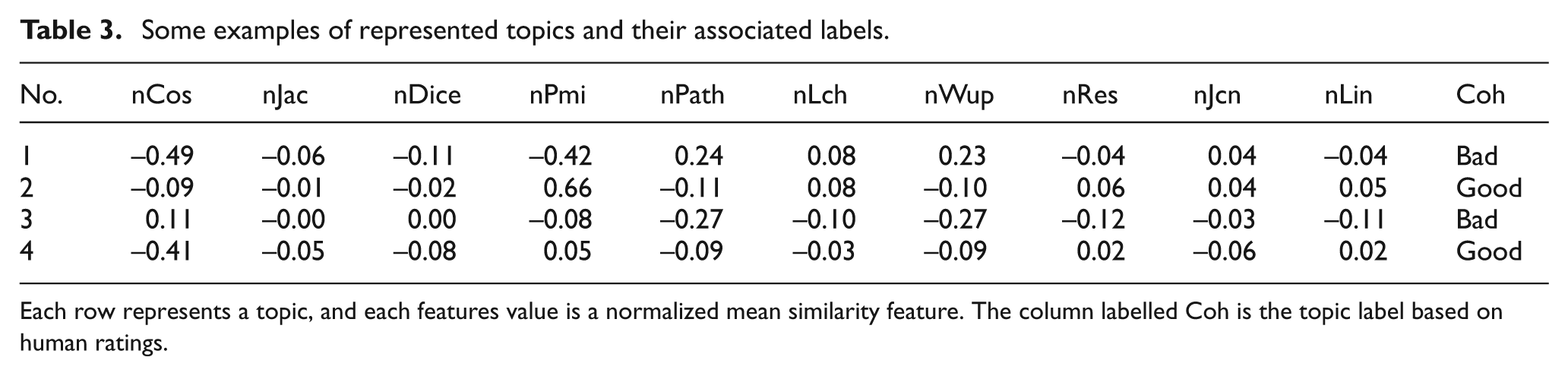
Each row represents a topic, and each features value is a normalized mean similarity feature. The column labelled Coh is the topic label based on human ratings.

Figure 1.

Proposed methodology to evaluate represented topics.

3.1. Pre-processing

We used two types of English corpora (Table 1) from news domains: United Press International (UPI) and Reuters. We downloaded 168,016 UPI news articles¹ and randomly selected 10,000 pages, naming it UPICorpus. The Reuters corpus is from Python’s natural language toolkit (NLTK), originally divided into training and test sets, and combined into ReutersCorpus. We used lower-case alphabetic words of lengths 3–25, and removed stop words using Rapid Miner’s Filter stopwords (English) operator and NLTK’s stopwords corpus. Words were lemmatized using NLTK’s WordNet lemmatizer, and retained noun sense if more than one sense exists. We pruned the words that appeared in fewer than 2% of UPICorpus (1% of ReutersCorpus) and more than 90% of the documents.

3.2. Latent Dirichlet allocation

LDA [9] is a generative topic model that assumes that documents are mixtures of topics, and a topic is a distribution over a fixed vocabulary. LDA outputs topic representations of each document and the words associated with each topic. We used a Matlab implementation of LDA [10] available online.² We set the number of topics (120 for UPICorpus and 150 for ReutersCorpus), $α = 0.5 and β = 0.01$ . In addition to text mining and informational retrieval, topics are useful in certain applications [11] where topics are used as features to improve the classification algorithm AdaBoost.MH.

In equation (1), T is an ordered collection of k topics inferred through LDA using the toolbox downloaded from the link listed in Note 2. Each topic in T has the same vocabulary words but in a different order (at least two words if not all). In equation (2), $T^{r}$ is the rth topic in T having top-m (m = 10) words, where the word $w_{1} \in T^{r}$ has the highest probability of occurrence in it.

T = (T^{1}, T^{2}, \dots, T^{k})

(1)

T^{r} = {(w_{1}, w_{2}, w_{3}, \dots, w_{m})}^{r}; r = 1, 2, \dots, k

(2)

3.3. Word similarities and topic representation

We used two types of word similarities,³ thesaurus- and corpus-based. Thesaurus-based algorithms measure similarity by seeing words in hypernym hierarchies or words that have similar glosses (definitions). Corpus-based algorithms calculate words’ similarities using distributional contexts.

Equation (3) represents an ordered collection of word similarities in general and is concretely specified in equation (4), where F is a 10-tuple of word similarity features used in this article. All 10 similarity measures listed in equation (4) are discussed in following subsections (see Sections 3.3.1 and 3.3.2).

F = (F_{1}, F_{2}, \dots, F_{n})

(3)

F = (Cosine, Jaccard, Dice, PMI, Path, Lch, Wup, Res, Jcn, Lin)

(4)

We treated an rth topic $T^{r}$ as an object and represented it via mean values of pair-wise word similarity features $F_{i}$ , see equations (5)–(7).

Let,

T_{rep}^{r} = r^{th} represented topic

(5)

Equation (6) shows general formula to combine pair-wise word similarity scores. In equation (6) the denominator c is a binomial coefficient to find the number of unique word pairs associated with a topic $T^{r}$ and it is 45 for each 10 word topic $T^{r} .$ Associated with word similarity $F_{i}$ the mean in equation (6) was calculated differently for different types of features. Thesaurus-based similarities provide a single score for each word pair and their mean is a simple mean formula as in equation (6). For WordNet-based features we calculated mean similarity by following equation (10).

\begin{matrix} mSi m_{F_{i}} = \frac{\sum_{i = 1, j = 1 (k > i)}^{c} {(w_{i} w_{k})}^{r} . F_{i}}{c} \\ where c = (\begin{matrix} m \\ 2 \end{matrix}) = 45 at m = 10, and w_{i}, w_{k} \in T^{r}, i = 1, 2, \dots, n \end{matrix}

(6)

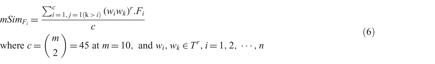
Equation (7) shows representation of topics by mean values of word similarity features. Following the order of equation (4), the first value of the n-tuple in equation (7) is associated with the Cosine similarity measure (see equation 8) and the nth (=10) value is associated with the Lin similarity measure (see equation 9).

T_{rep}^{r} = (mSi m_{F_{1}}, mSi m_{F_{2}}, \dots, mSi m_{F_{n}}) for r = 1, 2, \dots, k

(7)

\begin{matrix} {(w_{i} w_{k})}^{r} . F_{1} = Cosine {(w_{i}, w_{k})}^{r} \\ Cosine similarity between words w_{i} and w_{k} \end{matrix}

(8)

\begin{matrix} {(w_{i} w_{k})}^{r} . F_{n} = Lin {(w_{i}, w_{j})}^{r} \\ Lin similarity between words w_{i} and w_{k} \end{matrix}

(9)

3.3.1. Thesaurus-based similarities

Like a thesaurus, WordNet is a lexical database of words where nouns, verbs, adjectives and adverbs are grouped into sets of synonyms (synsets), each uttering a different concept. In addition to this, the WordNet labels semantic relations among words and interlinks specific senses by means of semantic and lexical relations. It is a great resource for word sense disambiguation and other computational work in natural language processing and information retrieval.

We used the WordNet interface⁴ provided by the NLTK for six WordNet-based word similarity features divided into two categories: path-based (equations 11–13) and information content-based similarities (equations 14–16). Let us define some terminologies used in these features definitions. Least common subsumer (LCS) is a lowest node in the WordNet hierarchy that subsumes two word senses, synset1 and synset2. P(synset1) is the probability that a randomly selected word in a corpus is an instance of synset1. The information content of synset1, IC(synset1), is –log(P(synset1)). We created the information content dictionary separately for each corpus.

WordNet similarity algorithms apply to pairs of synsest rather than to word pairs. To assign a single similarity score for a word pair (of a topic), we searched each pair of words in WordNet and exhaustively generated similarity scores for each sense of $w_{i}$ with each sense of word $w_{k}$ and then took the mean value (see equation 10). If a word was absent in WordNet its score was zero.

mWordNetSim (w_{i}, w_{k}) = \frac{\sum_{synset 1 \in senses (wi), synset 2 \in senses (wk)} WordNetSim (synset 1, synset 2)}{| senses (wi) |}

(10)

Path Similarity (Path): Path(synset1,synset2) returns the number of nodes in the shortest path that connects the two senses in the hypernym/hyponym relation and it provides a score in the range 0–1. The path length of the sense with itself is 1.

Path (synset 1, synset 2) = \frac{1}{1 + no . of edges in the shortest path in hypernym graph between two senses}

(11)

Leacock Chodorow Similarity (Lch): this was proposed by Leacock et al. [12]. It is based on the shortest path length (p) between two senses and the maximum depth (d) of the taxonomy in which the senses occur.

Lch (synset 1, synset 2) = - \log (\frac{p}{2 d})

(12)

Wu Palmer Similarity (Wup): this is based on the depth of the two senses in the taxonomy and that of their least common subsumer (most specific ancestor node) [13].

wup (synset 1, synset 2) = \frac{2 \times depth (LCS (synset 1, synset 2))}{depth (synset 1) + depth (synset 2) + 2 \times depth (LCS (synset 1, synset 2))}

(13)

Resnik Similarity (Res): the more two words have in common, the more similar they are. According to Resnik [14], the information content of the most informative (lowest) subsumer (MIS/LCS) of the two nodes is defined as follows:

Res (synset 1, synset 2) = - \log (P (LCS (synset 1, synset 2)))

(14)

Jiang Conrath Similarity (Jcn): this is based on the information content (IC) of the least common subsumer and that of the two input synsets [15].

Jcn (synset 1, synset 2) = \frac{1}{IC (sunset 1) + IC (sunset 2) - 2 \times IC (LCS (synset 1, synset 2))}

(15)

Lin Similarity (Lin): Lin [16] altered the formula of Resnik:

Lin (synset 1, synset 2) = \frac{2 \times \log (P (LCS (synset 1, synset 2)))}{\log (P (synset 1)) + \log (P (synset 2))}

(16)

3.3.2. Corpus-based similarities

There are some problems with thesaurus-based meaning. We do not have a thesaurus for every language and if it exists we may have problems with recall; that is, many words and/or phrases may be missing and connections between senses may be missing too. Thesauri work less for verbs and adjectives because adjectives and verbs have less structured hyponymy relations. Distributional algorithms find similarity based on similar distributional contexts. Distributional algorithms⁵ also called vector-space models of meaning and offer much higher recall than hand-built thesauri but tend to have lower precision. The distributional algorithms work on the principle that two words are similar if they have similar word contexts.

We used four corpus-based distributional similarities: Cosine, Jaccard, Dice and PMI. The first three (Cosine, Jaccard and Dice) are based on a term document matrix and PMI was calculated using bigram collocations of window size 5. Each cell of a term document matrix had a TF-IDF value instead of raw frequencies and the two words $w_{i}$ and $w_{k}$ are similar if their vectors v and w are similar in terms of following similarities.

Cosine (v, w) = \frac{v . w}{| v | | w |} = \frac{v}{| v |} . \frac{w}{| w |} = \frac{\sum_{i = 1}^{n} v_{i} w_{i}}{\sqrt{\sum_{i = 1}^{n} {v_{i}}^{2}} \sqrt{\sum_{i = 1}^{n} {w_{i}}^{2}}}

(17)

Jaccard (v, w) = \frac{\sum_{i = 1}^{n} \min (v_{i}, w_{i})}{\sum_{i = 1}^{n} \max (v_{i}, w_{i})}

(18)

Dice (v, w) = \frac{2 \sum_{i = 1}^{n} \min (v_{i}, w_{i})}{\sum_{i = 1}^{n} (v_{i} + w_{i})}

(19)

We calculated PMI⁶ using bigrams with window size 5 and use term frequencies based on our local corpora. According to Church and Hanks [17] the PMI defines whether the two words $w_{i}$ , $w_{k}$ co-occur more than if they are independent.

PMI (w_{i}, w_{k}) = lo g_{2} \frac{P (w_{i}, w_{k})}{P (w_{i}) P (w_{k})}

(20)

3.4. Coherence-based topic annotations

All annotators were from countries where the official language is English and each had at least a master’s degree. Each person was spoken to one-on-one to clarify the written instructions about topic annotations. A topic was coherent if one can easily assign a heading to it otherwise incoherent. See Table 2 for some examples of coherent (Good) and incoherent (Bad) topics. In addition to the binary ratings we also collected topic titles and five scale ratings. By careful investigation (seeing the mean value of topic coherence mCoh, topic titles and five scale ratings) we set topic labels as Good (coherent) and Bad (incoherent) based on a majority vote. For the UPICorpus (120 topics) we set those topics as Good in which at least five (out of seven) ratings were 1, otherwise we labelled the topic Bad. It gave us 64 Good and 56 Bad topics, a nearly balanced number of labels. For the ReutersCorpus (150 topics) we employed four raters. Topics based on ReutersCorpus were more ambiguous than the UPICorpus and in most of the topics the starting three to five words were somewhat relevant, so we set topics as Good in which all the ratters agreed and we set topics as Bad in which at the most two ratters agreed about goodness. To make the number of Good/Bad topics balance we rejected 41/150 ReutersCorpus topics that do not follow the criteria and we were left with 110 topics: 52 Good and 58 Bad. Finally, the UPICorpus and ReutersCorpus had 120 and 110 topics respectively with 64 and 52 Good topics and 56 and 58 Bad topics, respectively.

To judge inter-annotator agreement we applied Fleiss’s kappa [18] (hereafter kappa). Kappa gives a value of 1 if the annotators are in complete agreement and $\leq 0$ if there is no agreement at all between the annotators. For UPICorpus, kappa was 0.21 and it was 0.27 for ReutersCorpus (a fair agreement according to Landis and Koch [19]).

3.5. Classification of represented topics

In this section we discuss the preparation of two datasets, classification algorithms and the evaluation strategy for these binary classifiers. Our datasets (UPI or Reuters) have records (Section 3.5.1) belonging to one of two topic classes (Good or Bad) and the objective was to design an automatic topic coherence model that could predict whether a query topic is Bad (incoherent) or Good (coherent). In our work, we used three state-of-the-art supervised classification algorithms; Random Forest, Support vector machine (SVM) and K-nearest neighbour (K-NN). According to Fernández-Delgado et al. [20], amongst 179 classifiers, Random Forest versions were found to be best followed by SVM. For Wu et al. [21], SVM and K-NN along with tree algorithms (C4.5, CART) were classified amongst the top data-mining algorithms. For details about SVM, K-NN and the tree algorithms read Wu et al. [21] and for Random Forest read Breiman [22].

We used Rapid Miner Studio 6.1 to perform topic classification (see Section 4.1) and evaluation. The following subsections specify parameter settings for different Rapid Miner operators, aiming at the reproducibility of results (Table 4) and we will publicly share all of the datasets and corpora used here. For the root operator (in all six classification experiments) we set the parameter random seed (= 2015) and other parameter values were default.

Table 4.

Supervised classification of represented topics: average precision, recall and accuracy percentages on two datasets based on 10-fold cross-validations.

Evaluation	UPI SVM	Reuters SVM	UPI Random Forest	Reuters Random Forest	UPI 11-NN	Reuters 5-NN
Precision_Good	83.08	77.36	82.35	73.02	80.28	72.22
Recall_Good	84.38	78.85	87.50	88.46	89.06	75.00
Precision_Bad	81.82	80.70	84.62	87.23	85.71	76.79
Recall_Bad	80.36	79.31	78.57	70.69	75	74.14
Accuracy	82.50 ± 10.83 micro:82.50	79.09 ± 8.18 micro:79.09	83.33 ± 8.33 micro:83.33	79.09 ± 11.54 micro:79.09	82.50 ± 8.70 micro:82.50	74.55 ± 8.91 micro:74.55
meanRecall	82.21 ± 10.90 micro:82.37	78.83 ± 8.57 micro:79.08	82.93 ± 8.59 micro:83.04	79.33 ± 11.31 micro: 79.58	81.81 ± 8.57 micro:82.03	74.17 ± 8.92 micro:74.57
meanPrecision	84.96 ± 10.06 micro:82.45	80.55 ± 8.75 micro:79.03	85.24 ± 8.20 micro:83.48	80.71 ± 11.79 micro: 80.12	86.75 ± 6.63 micro:83.00	76.27 ± 9.87 micro:74.50

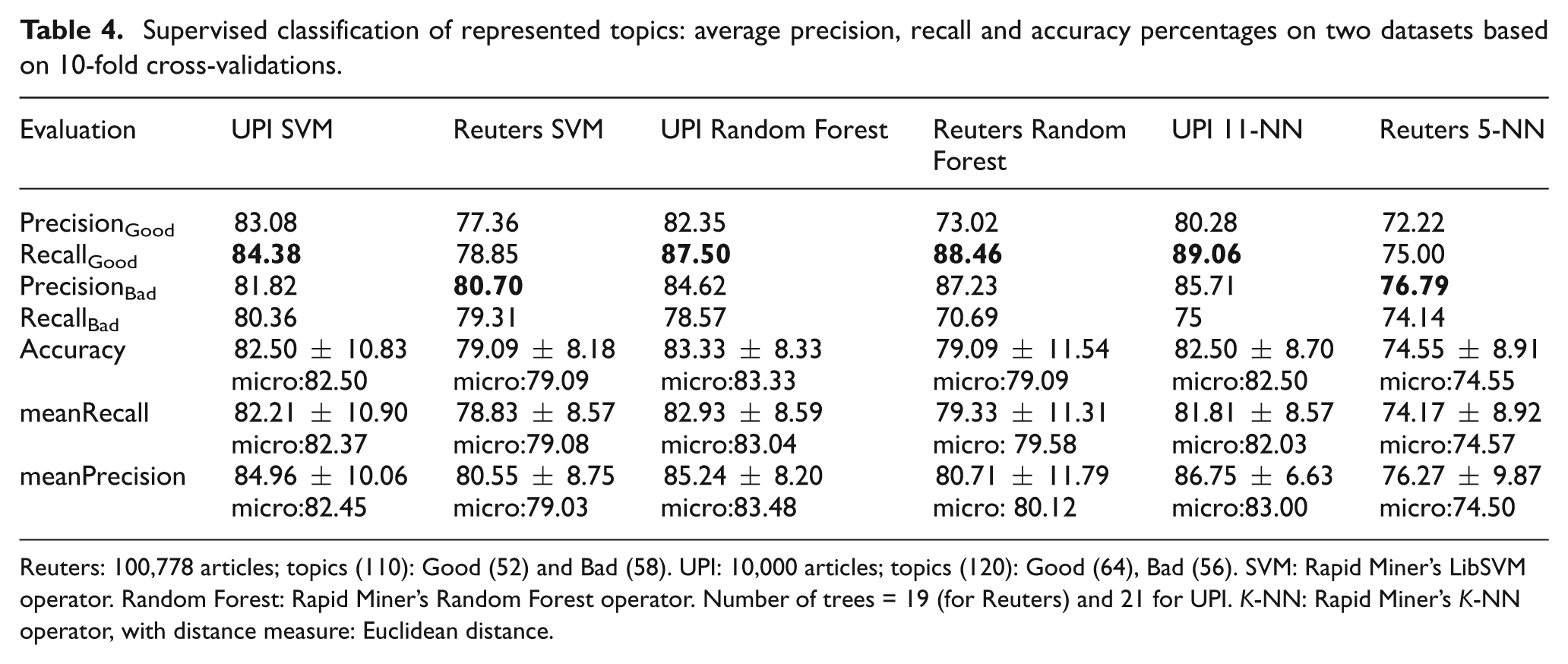
Reuters: 100,778 articles; topics (110): Good (52) and Bad (58). UPI: 10,000 articles; topics (120): Good (64), Bad (56). SVM: Rapid Miner’s LibSVM operator. Random Forest: Rapid Miner’s Random Forest operator. Number of trees = 19 (for Reuters) and 21 for UPI. K-NN: Rapid Miner’s K-NN operator, with distance measure: Euclidean distance.

3.5.1. Datasets

We prepared two datasets UPI and Reuters for the two corpora. First, for each corpus we now have topics (120 for UPICorpus and 110 for ReutersCorpus) and their associated labels (see Table 2, last column). Second, we represented each topic by mean values of pair-wise word similarity features following equation (7). Third, using represented topics and their corresponding labels we prepared two tables. Finally, we performed data normalization for each table separately and obtained two datasets: UPI and Reuters. Table 3 shows four represented topics (from Table 2) with normalized mean values of word similarity features along with topic labels. After normalization (equation 21), all features were on the same scale with zero mean and unit variance. In equation (21), $μ$ is the mean of feature $F_{i}$ , and $σ$ is standard deviation:

n Sim = \frac{mSi m_{F_{i}} - μ}{σ}

(21)

3.5.2. Random Forest

We used Rapid Miner’s Random Forest operator to perform topic classification. It generates a set of a specified number of random tree models, and the resulting model is a voting model. While training the classifier, we allow pruning (prepruning) to avoid over-fitting. Keep in mind that, for the reproducibility of results, we are reporting all parameters settings of the Random Forest operator for UPI (Reuters) dataset-based experiments. Number of trees = 21(19); 21 trees worked best for UPI and 19 for Reuters. Criterion = gain_ratio for both datasets is an entropy measure used to select attributes for splitting during the tree-building process and it adjusts information gain values for each attribute to avoid bias towards attributes. Minimal size for split = 4 for both datasets; the size of a node is the number of examples in its subset and only those nodes are split where size is ≥4. Minimal leaf size = 3(2); 3 for UPI and 2 for Reuters. Every leaf node subset has at least the minimal leaf size number of instances. Minimal gain to split a node = 0.1. Maximal depth = −1; to impose no bound on the depth of a tree. Confidence = 0.1; confidence level used for the pessimistic error calculation of pruning. Number of prepruning alternatives = 10; prepruning runs parallel to the tree-generation process and it may prevent splitting at certain nodes when splitting at that node does not add to the discriminative power of the entire tree and this parameter adjusts the number of alternative nodes tried for splitting when a split is prevented by prepruning at a certain node. Guess subset ratio = true for the UPI dataset only, and for Reuters it was set to false, so we chose subset ratio = 1.0 for the Reuters dataset only and it was the ratio of randomly chosen attributes to test. To produce the same randomization again and again we set local random seed as 2001.

3.5.3. Support Vector Machine

An SVM classifies data by finding the best hyperplane (the plane having the largest margin between two categories) that separates all data points of one class from those of the other classes. Margin means the maximal width of the slab parallel to the hyperplane that has no interior data points. We used the support vector machine (LibSVM) operator of Rapid Miner. This operator is an SVM learner, based on the Java LibSVM⁷ by Chang and Lin [23]. Their paper discusses the solution of SVM optimization problems and parameter selection for LibSVM in a comprehensive way. Built-in help associated with the Random Forest operator in Rapid Miner is also sufficient to use this operator.

For the UPI (Reuters) datasets the parameter settings of the Rapid Miner operator LibSVM are written in the following lines: svm type = nu-SVC; kernel type = rbf; gamma = 0.1(0.2); nu = 0.5(0.4); cache size (in megabytes) = 80; epsilon (tolerance of the termination criterion) = 0.01. The attributes shrinking, calculate confidences and confidence for multiclass were all set to true (these have no impact on Reuters results, but without these we lost 1% of accuracy with the UPI dataset). In our experiments the choice of the kernel type as rbf and setting the gamma and nu values were very crucial.

3.5.4. K-nearest neighbour algorithm

Given dataset D of n represented topics, $T_{rep}^{r}$ , and a distance function, K-NN finds the k closest topics in D to a query topic. We used Rapid Miner’s K-NN operator with a Euclidean distance measure, and we experimented with different values of k =1, 3, 5, …, 25, to find the best number of neighbours (k). For UPI the best k was 11 and it was 5 for Reuters.

3.5.5. Validation of binary classifiers

We used 10-fold cross-validation to estimate the generalization error of the three predictive models. In k-fold cross-validation the training dataset was divided into k equal-sized subsets. The result of the k-fold cross-validation is the average of the performances obtained from the k rounds. From Rapid Miner we used the X-Validation operator to estimate the statistical performance of Random Forest, LibSVM and K-NN. For all the experimental results (Section 4.1), we used fixed parameter settings of this operator: average performances only = true; number of validations = 10; sampling type (to build the subsets) = stratified_sampling.

4. Results and discussion

The experiments were performed on two datasets, UPI and Reuters, both belonging to the news domain. Note that over the passage of time the utilization of words may change, and a change of news agency or author also impacts writing style. The use of abbreviations and the presence of large numbers of numeric data in the documents affects the inferred topic interpretations. The nature of articles (their subjects) also influences the choice of words or numeric elements. Although the choice of top-m words for a topic affects its interpretability we just followed the norm [1 –7] and used the top-m (m = 10) words of a topic. In most of the related papers either the top-5 or the top-10 words have been used. In reality the choice of the top-m words should be very careful, and the choice of the top-m words may vary from topic to topic, keeping in mind that LDA does not always give a perfect ordering of the words. That is, the choice of m for different topics may be different and not constant. For each topic, m can be treated as a random variable, M, and it can be 5, 10, 12, …, depending on the interpretability. How we can automate this M is something we want to tackle in our future work. Kappa values for UPI and Reuters were found in fair agreement as suggested by Landis and Koch [19]. Low values of kappa (UPI = 0.21 and Reuters = 0.27) suggest that annotators did not quite agree with each other, as observed by Röder et al. [5], and the reason may be that the most probable top words were ambiguous as to interpretation [8].

In our surveys (see Section 3.4) the collection of topic titles and five scale ratings along with binary labels has several objectives. First, topic titles and five scale rating may be helpful for annotators to take strict (two-level) ratings for topic coherences. For example, seeing rating 4 or 5 and the presence of topic title, an annotator can surely be confident in assigning a Good label to a coherent topic. Second, we assigned binary labels (as discussed in Section 3.4) to topics using the automatic majority vote method (we also considered mode for automatic topic labels but found the majority method more useful by manual analysis of topics and automatic topic labels) and to authenticate their quality we checked the presence (or absence) of topic title and high/low five scale rating. Third, the five scale ratings are also helpful to investigate the classification results (see Section 4.1.1 and Table 5). Fourth, the presence of topic titles and five scale rating will be helpful for our future work and also make our surveys complete in the sense that these will be more resourceful to potential users as we also want datasets that are publicly available.

Table 5.

Examples of misclassified topics over UPI dataset with 70% training data and 30% test data.

Topics	Y	Y′	Y′′	Y′′′	Vote
1 − help work make improve good create keep focus look approach	1	0	0	0	5
2 − state florida saturday texas miami defeat sunday thursday friday west	0	1	1	1	1
3 − find say body discover investigator determine dead death release investigate	1	0	1	0	5
4 − test data target information include provide develop conduct range monitor	1	1	1	0	5
5 − thursday schedule park expect wednesday begin night report attend delay	1	1	1	0	6
6 − system contract defense support technology provide capability advance solution service	0	1	1	1	4
7 − good know see look lot bad thing time happen get	0	0	0	1	3
8 − program martin part deliver director include provide partner statement development	0	0	0	1	2
9 − run strike start hit loss lead give throw bring take	0	0	0	1	4
10 − billion estimate street wall journal total million deal cost major	0	1	1	1	3
11 − member issue review association standard approve propose limit measure consider	0	1	0	1	3

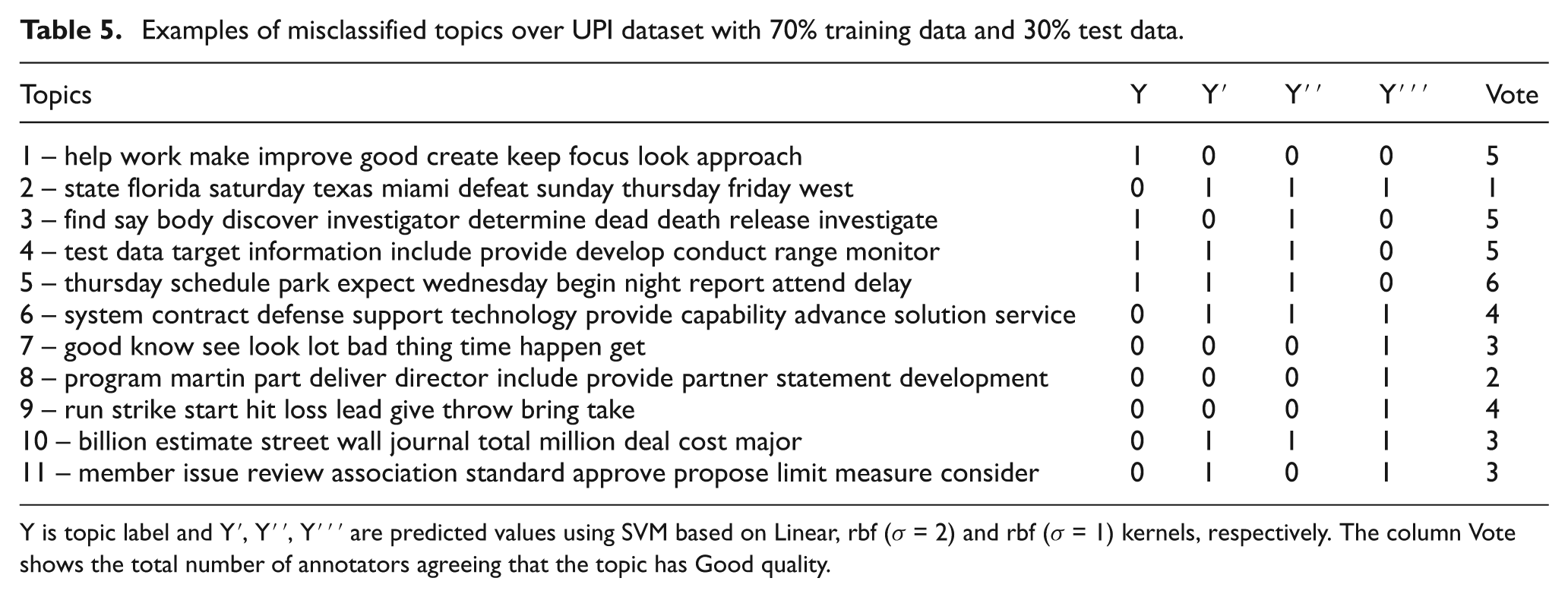
Y is topic label and Y′, Y′′, Y′′′ are predicted values using SVM based on Linear, rbf (σ = 2) and rbf (σ = 1) kernels, respectively. The column Vote shows the total number of annotators agreeing that the topic has Good quality.

4.1. Binary classification of topics

Each row in the datasets represents a topic; each column has normalized mean values of pair-wise word similarity features and the final column of the datasets (see Table 3) has binary labels. We evaluated binary classifiers (see Section 3.5.5) by 10-fold cross-validation to avoid over-fitting. We used different performance metrics (precision, recall and accuracy) to show the quality of the auto-decision-making of the three classifiers on two datasets, making the total number of experiments six. Using four entries of confusion matrices for each iteration of 10-fold cross-validation (true positive, true negative, false positive and false negative), we show results in Table 4. The aggregate confusion matrix was constructed by evaluating different models on different test subsets during the 10 iterations of cross-validation. In Table 4 the first four rows (below the header) represent precision and recall percentage of each class of topics (Good/Bad) using the aggregate confusion matrix. The fifth to seventh rows of Table 4 are based on two types of averages: macro average (macro), which is the mean of all 10-fold averages; and micro average (micro), which is based on the aggregate confusion matrix. In the fifth row, the second column (named UPI SVM), 82.50 is the arithmetic mean (macro) of the accuracies obtained from the 10 rounds with a standard deviation of 10.83 followed by a micro average (82.50) computed from the aggregate confusion matrix. The differences between the two averages can be large; macro-averaging gives equal weight to each fold whereas micro-averaging gives equal weight to each per-topic classification decision. Micro-averaged results are a measure of effectiveness on the large classes in a test collection, whereas macro-averaged results provide a sense of effectiveness on small classes. Because the datasets are quite balanced, Table 4 (rows five to seven) has macro and micro averages that are the same or nearly equal to each other.

K-NN is a very simple algorithm but was found to be comparable to the other two algorithms. With the UPI dataset, the results are good but it performed poorly with the Reuters dataset. In all of the experiments the Reuters-based evaluation results were low compared with UPI and the reason for this may be the nature of the ReutersCorpus. According to our analysis of both corpora, ReutersCorpus articles have more word contractions (e.g. the use of both ‘avg’ and ‘average’ in the ReutersCorpus was found in high frequency, whereas in UPI we only found the use of ‘average’). ReutersCorpus also has more numerical data, compared with the UPICorpus, and also has many words that belong to far fewer documents, thus affecting the topics’ interpretability. LDA topics based on the Reuters dataset were also found to be more ambiguous and difficult to rate as compared with UPI-based topics. The K-NN algorithm is always sensitive to local data and it is advisable to search for the best K (the number of nearest neighbours). For example, for our UPI dataset the classification accuracy fluctuated from 73 to 83% and the 10-fold classification error was highest (0.27) at k = 1 and lowest (0.17) at k = 11. Similar behaviour was also found with the Reuters dataset. Further note that, finding the best k for K-NN algorithm is also termed as training the model.

Random Forest classifiers were the best performers (also identified by Fernández-Delgado et al. [20]), showing high averages in accuracy, recall and precision. We carefully analysed all tree models of random trees generated over both datasets. For UPI, a maximum of three features (PMI, Wup, path) were utilized in all of the tree models; 19 (out of 21 tree models over UPI) used PMI as a root attribute node; and only two models used Wup similarity as the root. In five models, the path length feature in combination with PMI (as root) and/or with Wup was found. In short, for UPI, PMI was the best feature, Wup second best, and the path-based feature was the third and last prominent feature. For Reuters, the results showed the use of all features in the tree models; in 19/19 random trees, PMI was the root node, and the second node to the root node was either Wup or Path, again showing the dominancy of these three features in the model building process. It looks like the combination of the thesaurus-based feature (specifically PMI) with WordNet features (specifically Wup or Path) makes a good combination for high performance.

We performed experiments with three different types of topic representations schemes and only reporting the results of best representation (see Table 3). To combine pair-wise similarity scores associated with each word pair we experimented with normalized mean (as in Newman et al. [1]) and normalized sum. Table 3 shows an instance of dataset (10 input features); we preferred to show the results in this paper where each column is associated with the normalized mean value of a word similarity measure. Newman et al. [1] used mean and median for combining pair-wise similarity. They did not find any reason which one was better for combining the pair-wise scores and here we preferred (randomly) mean over median. We adopted the normalization of features values to minimize the impact of large valued features but may have less discrimination power. In Newman et al. [1] there was no need to use normalized scores since they used correlation coefficient (see Tables 2 and 3 in Newman et al. [1]) as correlation gives similar results for both normalized and non-normalized data. Let us talk about the other two representation schemes (results are not shown here), where in one of the representations each column was normalized with individual scores of word pairs associated with a single similarity feature (rather than combining them into a single score), and in another representation scheme each column represents a word pair (rather than whole topic) having a sum of similarity scores associated with that pair. In the later representation scheme we see better classification performance of up to 82% classification accuracy and in the former representation scheme classification accuracy did not exceed 75%. It is a good idea to compare the effects of applying different quantitative measures to combine similarity scores such as max (as defined by Dan Jurafsky⁸), min and variance alongside mean and media, and this comparison will be made in our future work.

4.1.1. Interpretation of misclassified topics

There can be multiple reasons for misclassification of topics. First, topic labels are not perfect (fair values of Fleiss kappa for both surveys related to the two corpora we used show that often the annotators do not agree with each other) and the reasons for this may be that the topics are wordy in nature; that some topics have bad quality; that words in the topics may have multiple senses and are ambiguous to interpret [8], being perceived differently by different annotators based on their views and/or background; that the presence of chain words as in Mimno et al. [2] may make life difficult for annotators; and finally (but not the final one), all of the topics may not be perfectly summarized by a single cut (as used in the literature [1 –7]) of using top-m words for all of the topics. Second, for any machine-learning task the choice of true or minimal set of features is crucial to learn a classifier and the presence/absence of a feature affects the classification. The presence of noisy features degrades the classifier accuracy. For example, we also experimented with UMass as an eleventh feature where classification performance was not improved in general rather than degrading for some of the classifiers, and because of this we did not report the classification results with UMass. This can be tackled by finding the right and complete combinations of features and will be addressed in a separate paper as further investigation is required to answer this question, which may come with adding other similarity measures and/or finding a minimal set of topic representative features. Third, seeing lower PMI correlation values for both of our corpora (see Tables 7 and 8) as compared with tables 2 and 3 of Newman et al. [1]), we hope that the use of local combined with external large corpora (as Wikipedia used in Newman et al. [1]) may improve the results. Fourth, the classifiers used in this paper are state of the art [20, 21] and all are strong enough (especially SVM and Random Forests) to classify with high accuracy provided that the records (topics) in the datasets have true representative features with true labels (topic coherence scores), but the proper choice of input parameters for classification algorithms is crucial. Here we did not focus on finding the best topic features but we did care about finding good input parameters for classification algorithms and in most cases we used an exhaustive approach.

Tables 5 and 6 are associated with three experiments that we performed to observe misclassified topics. We used the UPI dataset and randomly divided it into two sets: training and test. The training set had 84 records with 43 Good and 41 Bad topics, and the test set had 36 records with 21 Good and 15 Bad topics. We learned three classification models (using training set) using SVM with linear kernel (or dot product) and Gaussian radial basis kernel function (rbf), which require setting of the scaling factor sigma (σ), which is crucial. Table 5 shows all 11 misclassified topics of the test set where Y is the output label (bi-level coherence), whereas Y′, Y′′′ and Y′′′ are predicted values of the SVM classifier with three different settings and the final column Vote shows the number of annotators agreed about the Goodness of a topic (recall that we set Y (Coherence) equal to 1 (or Good) where at least five annotators were agreed else it is was set to 0 (or Bad)). In Table 6, the first two rows are associated with three confusion matrices showing all the four values – true positive (TP), true negative (TN), false positive (FP) and false negative(FN) – and the last three rows summarize the classification performance. Remember that we treated Good topics as positive examples. Note that the dominance of recall in Table 6 is associated with Good topics (and this also evident in Table 4), where false negatives are always fewer than false positives in all the three experiments. Also note that the change in parameters for a classifier affects its performance.

Table 6.

Confusion matrix and performance metrics of topics classification over UPI dataset with 70% training data and 30% test data.

	SVM linear kernel		SVM rbf kernel (σ = 2)		SVM-rbf kernel (σ = 1)
	Predicted Good	Predicted Bad	Predicted Good	Predicted Bad	Predicted Good	Predicted Bad
Actual Good	19 (TP)	2 (FN)	20 (TP)	1 (FN)	17 (TP)	4 (FN)
Actual Bad	4 (FP)	11 (TN)	3 (FP)	12 (TN)	7 (FP)	8 (TN)
Accuracy	83.33%		88.89%		69.44%
Precision_Good	82.61%		86.96%		70.83%
Recall_Good	90.48%		95.24%		80.95%

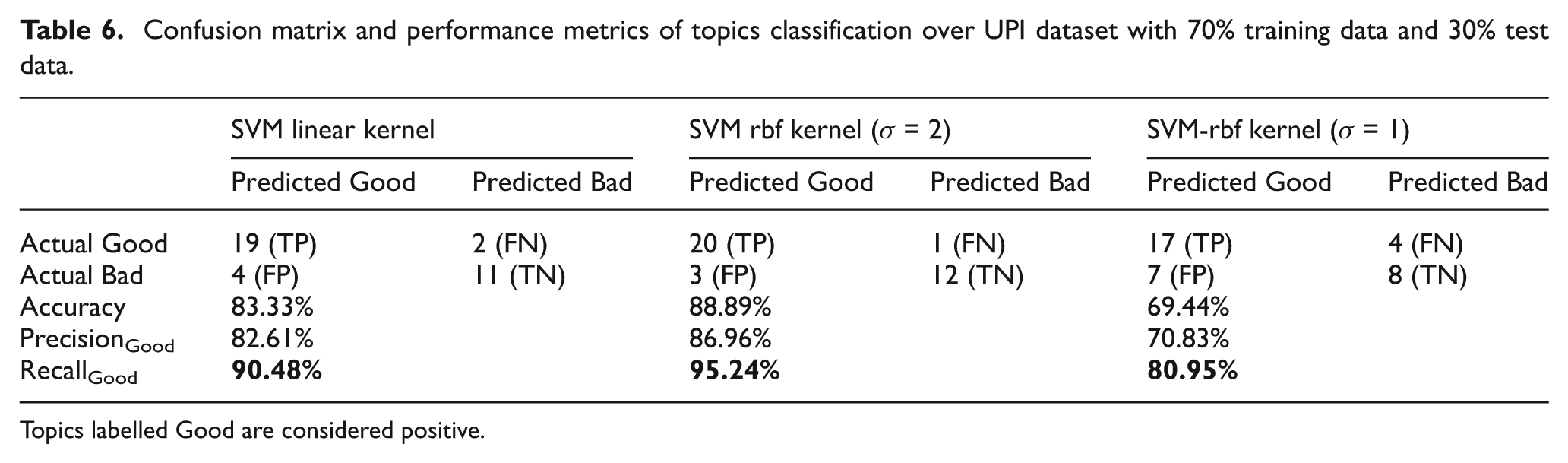
Topics labelled Good are considered positive.

In the test set we had 11 Good topics and four Bad topics, where six or all seven annotators were agreed and amongst the Good topics all were perfectly classified by SVM with linear and rbf (σ = 2) kernels but one topic (row 5 in Table 5) was misclassified by SVM with the rbf (σ = 1) kernel. Amongst the four Bad topics one (row 2) was misclassified by all of the classifiers. Combining these observations, we had only one topic (row 2 in Table 5) out of 15 (11 Good and four Bad) that was always misclassified, giving us 6.67% error. In topic 2 in Table 5, it looks as though it can be a candidate for being Good topic (but was assigned Bad by six annotators) since four words are week days (Saturday, Sunday, Thursday and Friday), four words are related to state (state, Florida, Texas and Miami), one word is related to direction (West), which can be associated with some states, and the last word is related to sports (defeat). Hence the concept of the topic (row 2, Table 5) may be related to sports between different states. All of the classifiers predict this topic as Good, but the label is Bad; this shows a very interesting case where features are more associated with word relatedness (but humans were choosing labels based on topic titles). This observation may guide us to explore some other features that may be more helpful to associate words with the general concept of the topic and/or we need to increase the window size for term context-based PMI features. In the test set (where at least two but fewer than six annotators were agreed about topic Goodness), there were 5/21, 3/21 and 9/21 topics for SVM with linear, rbf (σ = 2) and rbb (σ = 1) kernels that were misclassified, giving errors of respectively 23.8, 14.3 and 42.86%. In summary, topics where the majority of the annotators were agreed had less chance of misclassification and this is also an evidence (see also Table 4 for high classification results) that the topic representative features are faithful and are well associated with topic coherence. In other words we need to improve topic labels if we want to evaluate topics with high accuracy. This can be done by increasing the topic quality (by proper application of topic model) or by increasing the number of annotators. Low values of Fleiss kappa of our surveys also suggest that we need to improve the survey quality and this may be improved by utilizing experienced and/or paid (professional) annotators. Table 6 shows the confusion matrix and performance measures associated with Table 5.

4.2. Correlation between the descriptive features of a topic

Pearson’s correlation coefficient (correlation coefficients) is a normalized version of covariance and a dimensionless measure of linear dependence between two variables. Tables 7 and 8 show the correlation coefficients between topic labels (Coh), mean values of human ratings (mCoh), normalized mean values of word similarities and the coherence formula UMass [2]. High correlation between topic labels (Coh) and mean human ratings (mCoh) shows that our assignments of topic labels as Good (1) and Bad (0) using majority voting (see Section 3.4) is a rational approach.

Table 7.

Correlation coefficients over UPI dataset of 120 topics.

UPI	Coh	mCoh	UMass	nCos	nJac	nDice	nPmi	nPath	nLch	nWup	nRes	nJcn	nLin
Coh	1	0.88	0.33	0.32	0.33	0.34	0.55	−0.34	−0.21	−0.34	−0.16	−0.22	−0.16
mCoh	0.88	1	0.43	0.38	0.4	0.41	0.603	−0.32	−0.17	−0.31	−0.11	−0.17	−0.11
UMass	0.33	0.43	1	0.68	0.76	0.77	0.599	0.03	0.11	0.04	0.14	0.15	0.14
nCos	0.32	0.38	0.68	1	0.98	0.98	0.68	−0.02	0.08	−0.008	0.15	0.08	0.16
nJac	0.33	0.4	0.76	0.98	1	0.999	0.72	−0.05	0.05	−0.04	0.13	0.06	0.14
nDice	0.34	0.41	0.77	0.98	0.999	1	0.73	−0.05	0.06	−0.03	0.13	0.07	0.14
nPmi	0.55	0.6	0.599	0.68	0.72	0.73	1	−0.24	−0.07	−0.23	0.009	−0.08	0.01
nPath	−0.34	−0.32	0.03	−0.02	−0.05	−0.05	−0.24	1	0.85	0.999	0.78	0.82	0.77
nLch	−0.21	−0.17	0.11	0.08	0.05	0.06	−0.07	0.85	1	0.86	0.96	0.94	0.95
nWup	−0.34	−0.31	0.04	−0.008	−0.04	−0.03	−0.23	0.999	0.86	1	0.79	0.83	0.79
nRes	−0.16	−0.11	0.14	0.15	0.13	0.13	0.009	0.78	0.96	0.79	1	0.89	0.998
nJcn	−0.22	−0.17	0.15	0.08	0.06	0.07	−0.08	0.82	0.94	0.83	0.89	1	0.88
nLin	−0.16	−0.11	0.14	0.16	0.14	0.14	0.01	0.77	0.95	0.79	0.998	0.88	1

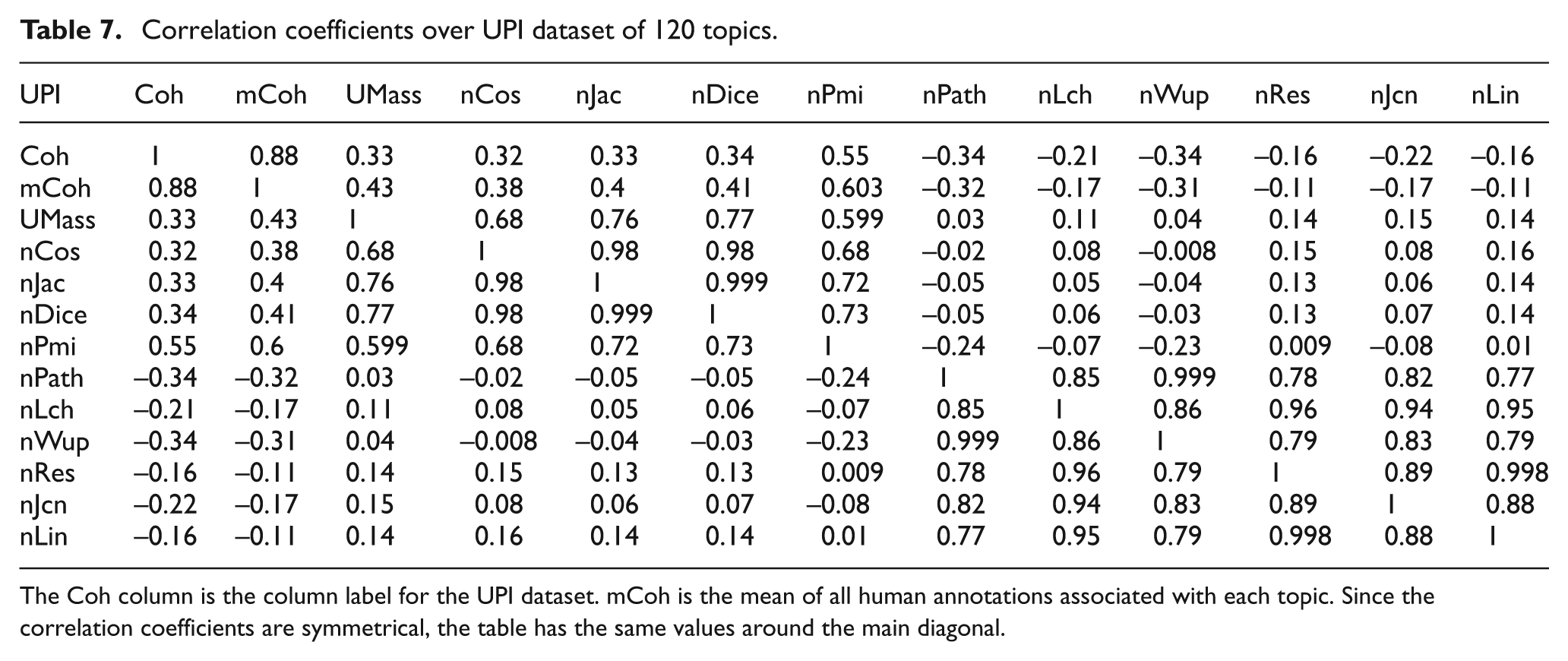
The Coh column is the column label for the UPI dataset. mCoh is the mean of all human annotations associated with each topic. Since the correlation coefficients are symmetrical, the table has the same values around the main diagonal.

Table 8.

Correlation coefficients over Reuters dataset of 110 topics.

Reuters	Coh	mCoh	UMass	nCos	nJac	nDice	nPmi	nPath	nLch	nWup	nRes	nJcn	nLin
Coh	1	0.92	0.21	0.17	0.14	0.18	0.47	−0.32	−0.26	−0.31	−0.12	−0.22	−0.08
mCoh	0.92	1	0.26	0.14	0.11	0.16	0.49	−0.37	−0.32	−0.36	−0.12	−0.26	−0.1
UMass	0.21	0.26	1	0.38	0.39	0.47	0.41	0.24	0.28	0.25	0.28	0.31	0.31
nCos	0.17	0.14	0.38	1	0.99	0.99	0.54	−0.2	−0.18	−0.2	−0.16	−0.17	−0.16
nJac	0.14	0.11	0.39	0.99	1	0.99	0.49	−0.18	−0.16	−0.18	−0.16	−0.15	−0.15
nDice	0.18	0.16	0.47	0.99	0.99	1	0.54	−0.16	−0.14	−0.16	−0.13	−0.13	−0.12
nPmi	0.47	0.49	0.41	0.54	0.49	0.54	1	−0.22	−0.18	−0.2	0.02	−0.16	0.02
nPath	−0.32	−0.37	0.24	−0.2	−0.18	−0.16	−0.22	1	0.94	0.998	0.77	0.92	0.78
nLch	−0.26	−0.32	0.28	−0.18	−0.16	−0.14	−0.18	0.94	1	0.94	0.8	0.96	0.82
nWup	−0.31	−0.36	0.25	−0.2	−0.18	−0.16	−0.2	0.998	0.94	1	0.8	0.94	0.81
nRes	−0.12	−0.12	0.28	−0.16	−0.16	−0.13	0.02	0.77	0.8	0.8	1	0.86	0.99
nJcn	−0.22	−0.26	0.31	−0.17	−0.15	−0.13	−0.16	0.92	0.96	0.94	0.86	1	0.87
nLin	−0.08	−0.1	0.31	−0.16	−0.15	−0.12	0.02	0.78	0.82	0.81	0.99	0.87	1

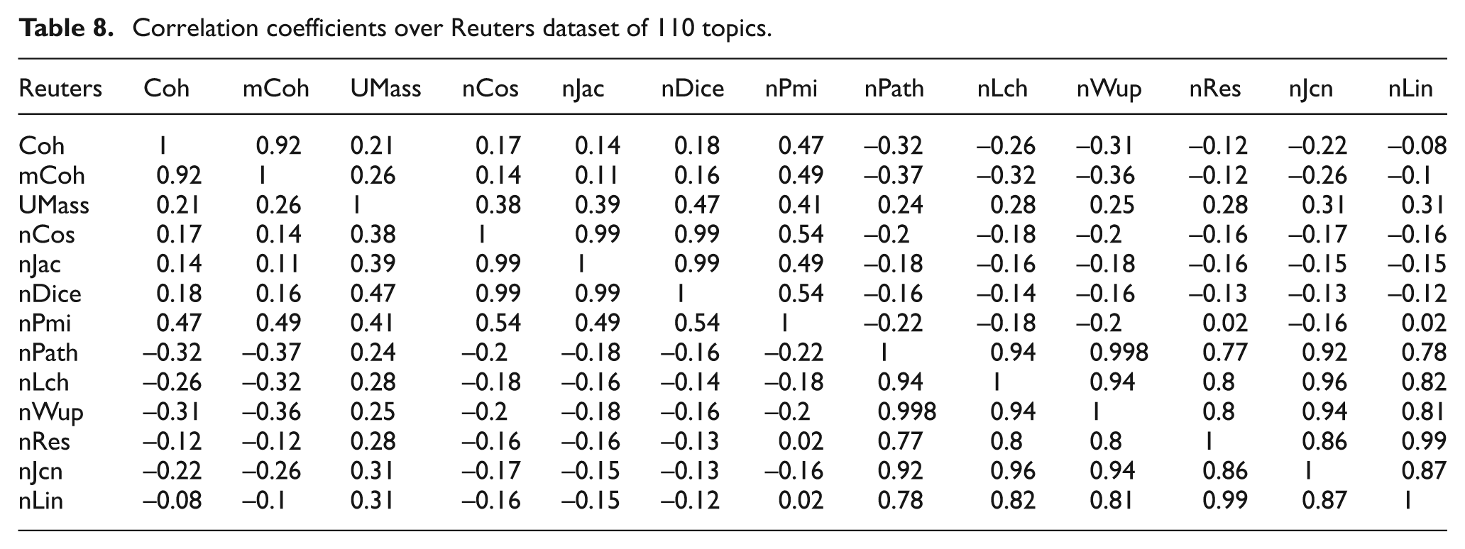
Consistent with the literature [1, 6], PMI is the most correlated with topic labels (Coh). With the increase in corpus size, it is expected that PMI will have higher correlation values. PMI has the highest correlation with output, so that is why it was a dominant feature in the Random Forest tree-building process. Each type of feature is highly correlated with the same type of features; that is, all thesaurus (WordNet)-based similarities were highly correlated with each other, and we also saw the same behaviour from corpus-based features. However, local corpus-based features were found to positively correlate to human ratings, whereas thesaurus-based features were found to negatively correlate, in general, as was also pointed out by Mimno et al. [2]. In our opinion, this opposite behaviour in two types of feature makes them complement each other, and their combination provided high classification performance; this is observed in tree models of the Random Forest algorithm (see Section 4.1). As for comparison between UMass and PMI, PMI had higher correlations with human ratings, proving its superiority for topic coherence over UMass, especially for smaller corpora.

Non-normalized feature values also gave the same correlation coefficients and that is why we are not using a normalized version of features. In general, correlation coefficients in Table 8 over the Reuters dataset show the same behaviour but some points are worth discussing. As we observed in Table 4, the Reuters-based classification performance was a little below par in comparison with UPI. In Table 8 the association of PMI with Coh and mCoh is smaller in comparison with that of UPI and the same is also true for other features in general. Here UMass (0.21) looks a little better than Cosine (0.17), Jaccard (0.14) and Dice (0.18), whereas in Table 7 Dice (0.34) is better than UMass (0.33). Here though the association between Coh and mCoh is higher (0.92) than that of UPI (0.88), but owing to less correlation strength between all word similarities and the topic label (Coh), the classification results were below par and the reasons for this may be the same as discussed in Section 4.1 (nature of the Reuters dataset).

Newman et al. [1] used Wikipedia (external corpus) for finding pair-wise word similarity scores and two local corpora to learn LDA topics. Following Mimno et al. [2], we use local corpora for both of the tasks. Although our local corpora are small as compared with [1, 2] and may lack coverage, observations about PMI and its highest correlation with human ratings is consistent with Newman et al. [1], amongst all the features, including WordNet-based measures for both of the datasets. In Tables 7 and 8, if we change the sign of path-based WordNet similarity correlations (Path, Lch and Wup; focus on the first row of both tables), then these three measures (especially Wup and Path) look more consistent than other corpus-based measures. These two features are also found in Random Forest ensembles, where Wup is second and Path is third to PMI, respectively in most of the tree models. These later observations differ a little from Newman et al. [1], where corpus-based features always outperform WordNet-based measures, provided we accept the change of sign for path-based correlation coefficients. Also note the dominance of Dice over Umass in Table 7 (see row 1).

4.3. Applications of topic representation scheme

One obvious application is to predict whether a topic is Good or Bad in terms of its coherence. This is significant when we want to run a topic model on the same corpus again and again to find the best k topics, and we do not have human annotations on each run. Once a topic classifier is trained, we can remove the human annotators from subsequent iterations, since human-based annotations are expensive and time-consuming and conflict with each other. The quantitative representation looks useful for finding automatic topic labelling, grouping similar topics into one cluster using unsupervised clustering algorithms. All of the applications of LDA topics can benefit from this representation, and this is the focus of our future work.

5. Conclusion

Our work is about topic representation via mean values of pair-wise word similarity features, and then evaluating whether the proposed topic representation scheme is faithful or not based on a topic coherence score. Using represented topics via mean values of pair-wise word similarity features, equations (1)–(9) and corresponding topic labels for each topic, we prepared two different datasets: UPI and Reuters. Based on these two datasets, we justified our topic representation scheme by performing the task of topic classification, and the results are shown in Table 4. Cross-validation-based classification performance suggests that the novel topic representation is associated with the topic coherence ratings, and this gives us confidence to further investigate other applications of our new perspective on tackling topics. Local corpus-based word similarities correlate positively with human ratings whereas thesaurus-based similarities were negatively correlated but their combination gave high topic classification performance. The correlation and classification results suggest that the two types of word similarities complement each other and their combination is helpful in developing classification models to predict topic coherence. It looks worthwhile to further investigate the proposed representation scheme by incorporating other similarity features and applying them to applications other than topic prediction.

Footnotes

Acknowledgements

The first author thanks Dr Seung Yeob Nam for his technical guidelines and Michael Röder for sharing the dataset used initially in the experiments, as well as all national and international friends who participated in the topic annotations survey.

Funding

This work was supported by Energy Efficiency and Resources Core Technology Program of the Korea Institute of Energy Technology Evaluation and Planning (KETEP) granted financial resource from Ministry of Trade, Industry & Energy, Republic of Korea (no. 20132010101800), for the first author. The work was also supported by Basic Science Research Program through the National Research Foundation of Korea, funded by Ministry of Science, ICT and Future Planning (2013-012524), for the second author. This work was supported by the 2014 Yeungnam University Research Grant for the fourth author.

Notes

References

Newman

Lau

Grieser

Baldwin

. Automatic evaluation of topic coherence. In: Human language technologies: The 2010 annual conference of the North American Chapter of the Association for Computational Linguistics, 2010, pp. 100–108.

Mimno

Wallach

Talley

Leenders

McCallum

. Optimizing semantic coherence in topic models. In: Proceedings of the conference on empirical methods in natural language processing. Stroudsburg, PA: Association for Computational Linguistics, 2011, pp. 262–272.

Aletras

Stevenson

. Evaluating topic coherence using distributional semantics. In: Proceedings of the 10th international conference on computational semantics (IWCS) – Long papers, 2013, pp. 13–22.

Rosner

Hinneburg

Röder

Nettling

Both

. Evaluating topic coherence measures. arXiv preprint, 2014, arXiv:1403.6397.

Röder

Both

Hinneburg

. Exploring the space of topic coherence measures. In: Proceedings of the eighth ACM international conference on web search and data mining (WSDM), 2015, pp. 399–408.

Lau

Newman

Baldwin

. Machine reading tea leaves: Automatically evaluating topic coherence and topic model quality. In: European Chapter of the Association for Computational Linguistics (EACL), 2014, 530.

Chang

Gerrish

Wang

Boyd-graber

Blei

. Reading tea leaves: How humans interpret topic models. In: Advances in neural information processing systems (NIPS), 2009, pp. 288–296.

Hinneburg

Rosner

Pessler

Oberländer

. Exploring document collections with topic frames. In: Proceedings of the 23rd ACM international conference on information and knowledge management (CIKM). New York: ACM, 2014, pp. 2084–2086.

Blei

Jordan

. Latent Dirichlet allocation. The Journal of Machine Learning Research 2003; 3: 993–1022.

10.

Griffiths

Steyvers

. Finding scientific topics. Proceedings of the National Academy of Sciences, 2004; 101(suppl. 1): 5228–5235.

11.

Al-Salemi

Ab Aziz

Noah

. LDA-AdaBoost. MH: Accelerated AdaBoost. MH based on latent Dirichlet allocation for text categorization. Journal of Information Science 2015; 41(1): 27–40.

12.

Leacock

Miller

Chodorow

. Using corpus statistics and WordNet relations for sense identification. Computational Linguistics 1998, 24(1); 147–165.

13.

Palmer

. Verb semantics and lexical selection. In: Proceedings of the 32nd annual meeting of the Association for Computational Linguistics (ACL’94), Las Cruces, New Mexico, 1994, pp. 133–138.

14.

Resnik

. Using information content to evaluate semantic similarity in a taxonomy. arXiv preprint, 1995, , arXiv: cmp-lg/9511007.

15.

Jiang

Conrath

. Semantic similarity based on corpus statistics and lexical taxonomy. arXiv preprint, 1997, arXiv: cmp-lg/9709008.

16.

Lin

. An information-theoretic definition of similarity. ICML July 1998; 98: 296–304.

17.

Church

Hanks

. Word association norms, mutual information, and lexicography. Computational Linguistics 1990; 16(1), 22–29.

18.

Fleiss

. Measuring nominal scale agreement among many raters. Psychological Bulletin 1971; 76(5): 378–382.

19.

Landis

Koch

. The measurement of observer agreement for categorical data. Biometrics 1977; 33: 159–174.

20.

Fernández-Delgado

Cernadas

Barro

Amorim

. Do we need hundreds of classifiers to solve real world classification problems? The Journal of Machine Learning Research 2014; 15(1): 3133–3181.

21.

Kumar

Quinlan

Ghosh

Yang

Motoda

. Top 10 algorithms in data mining. Knowledge and Information Systems 2008; 14(1): 1–37.

22.

Breiman

. Random forests. Machine Learning 2001; 45(1): 5–32.

23.

Chang

Lin

. LIBSVM: a library for support vector machines. ACM Transactions on Intelligent Systems and Technology 2011; 2(3): 27.