A study of neighbour selection strategies for POI recommendation in LBSNs

Abstract

Location-based recommender systems (LBRSs) are gaining importance with the proliferation of location-based services provided by mobile devices as well as user-generated content in social networks. Collaborative approaches for recommendation rely on the opinions of like-minded people, so-called neighbours, for prediction. Thus, an adequate selection of such neighbours becomes essential for achieving good prediction results. The aim of this work is to explore different strategies to select neighbours in the context of a collaborative filtering–based recommender system for POI (places of interest) recommendations. Whereas standard methods are based on user similarity to delimit a neighbourhood, in this work several strategies are proposed based on direct social relationships and geographical information extracted from location-based social networks (LBSNs). The impact of the different strategies proposed has been evaluated and compared against the traditional collaborative filtering approach using a dataset from a popular network as Foursquare. In general terms, the proposed strategies for selecting neighbours based on the different elements available in a LBSN achieve better results than the traditional collaborative filtering approach. Our findings can be helpful both to researchers in the recommender systems area and to recommender system developers in the context of LBSNs, since they can take into account our results to design and provide more effective services considering the huge amount of knowledge produced in LBSNs.

Keywords

Location-based social networks recommender systems

1. Introduction

Recommender systems (RSs) have become, during the last decade, an alternative to deal with the problem of information overload that users face when they are looking for information about items of interest in huge amounts of available data in a variety of domains such as tourism, movies, music and education, among others [1]. Several techniques have been developed to build RSs. Traditional techniques such as collaborative filtering (CF) and content-based (CB) recommendations process information obtained from the ratings provided by users to items and the characteristics of such items to generate a list of recommendations.

During the last years, there has been an increase in the use of cell phones and it has become easier to obtain information about the geographical location of people. These technological advances, as well as wireless communication, have facilitated the development of social services based on the geographical location of users. One of the most popular social networks of this kind is Foursquare,¹ which allows users to easily share their geographical location as well as contents related to this location in an online way. The user location is a new dimension in social networks that narrows the gap between the physical world and online social networking services, and provides new opportunities and challenges for traditional RSs [2].

In the context of social networks, RSs can take advantage of additional information such as users’ relationships and users’ behaviour in such networks [3]. Particularly, when considering location-based social networks (LBSNs), RSs can take into account geo-localised data of users to make recommendations. LBSNs allow users to build connections with their friends, share their locations via check-ins for points of interests (POIs, for example, restaurants, tourist spots, stores), as well as adding location-related contents (e.g. comments and geo-tagged photos). In addition to providing users a social interaction platform, LBSNs constitute a rich source of information to mine users’ preferences and open new possibilities for RSs.

Several location-based recommender systems (LBRSs) have emerged in recent years to recommend friends [4,5], activities [6,7], events [8,9] and places [10]. Given the variety of data contained in LBSNs, the need of developing new approaches for RSs that use different data sources and techniques to enhance recommendations has arisen. For example, the traditional CF method, which relates users to items through ratings or opinions provided by users, could be applied straightforwardly to build LBRSs. However, traditional CF considers neither the possible friendship relationships or the geo-localisation dimension.

In this work, we propose different strategies for including the additional information available in LBSNs for recommending POIs in the context of the CF approach. Particularly, we consider a user-based CF approach. User-based approaches recommend items (e.g. POIs) based on an aggregation of similar users’ (called neighbours) preferences. Since user-based CF trusts neighbours as information sources, the quality of recommendations depends directly on the ability to select these neighbours. Our hypothesis is that LBSNs provide rich information for establishing relationships beyond similarity, which can enhance the selection of potential neighbours and thus improve the estimation of preferences during the recommendation process. In addition, in LBSNs we can obtain user preferences from different sources, such as the visits of a user to a certain place and the tips or comments provided for the visited places.

The impact of the different strategies proposed has been evaluated using a dataset from Foursquare. The results obtained thus far indicate that some of the strategies analysed not only showed advantages over the baseline (i.e. pure CF approach) in terms of the prediction error for estimating user preferences but also in the number of comparisons needed when looking for neighbours as well as in the coverage reached for recommendations.

The remainder of the article is organised as follows. In section 2, we describe some related works. In section 3, we present our approach. In section 4, we present the experimental evaluation of the proposed approach. Finally, in section 5, we present our conclusions.

2. Related works

The recommendation of places is an important feature for LBSNs as it helps users discover and explore new attractive locations taking advantage of information provided by other users, including friendship relationships, check-ins on points-of-interest, comments, geographical information and categories of POIs. User-generated content in a social network provides rich knowledge to understand users’ interests and their relationships with others. In this context, RSs emerged as an alternative to mine actionable knowledge for prediction starting from LBSNs or even in traditional networks such as Twitter using location inference capabilities [11].

POI recommendation systems found in the literature stem from traditional techniques from the area of RSs such as CB, CF and hybrid approaches. Examples of CB RSs are LCARS [12], a location-content-aware recommender system that exploits the content information about a user preferred spatial items to produce recommendations in other cities, and the system proposed in Wang et al. [13] that explores text descriptions, photos, user check-in patterns and venue context for defining a location semantic similarity for venue recommendation. Context-aware recommendation is proposed in Bellotti et al. [6] for inferring possible leisure activities and recommends appropriate content on a site (shops, parks, movies). Park et al. [14] presented a recommendation system that reflects a user’s preferences modelled by Bayesian networks (BNs), inferring the most preferred items by collecting context information, location, time, weather and user requests from the mobile device. A hybrid content-aware CF approach is presented in Lian et al. [15] for addressing the cold-start problem.

CF approaches are based on a user-item matrix of ratings for assessing user preferences. LBRSs based on CF need to translate user check-ins into a user-item matrix, where each row corresponds to a user visiting history and each column is a POI. Users express their interests, which can be mapped to ratings to fill the matrix in several ways, ranging from explicit ones (e.g. starts) to implicit ones (e.g. comments or check-in frequency). LARS [16], a location-aware recommender system, deals with three types of location-based ratings: spatial ratings for non-spatial items, non-spatial ratings for spatial items and spatial ratings for spatial items. ORec [17] proposes an opinion-based POI recommendation framework that extracts the polarity of user opinions on POIs expressed as text-based tips. MARS (multi-aspect recommender system for POI) [18] is a multi-aspect user preference learning system that integrates ratings with reviews using Utility Theory. Matrix factorisation models are commonly used in CF approaches. For instance, Berjani and Strufe [19] applied a regularised matrix factorisation (RMF) technique for CF-based personalised recommendation of potentially interesting spots. GeoMF [20] incorporates into the factorisation model a spatial clustering phenomenon observed in human mobility behaviour on LBSNs. Context-awareness is also considered in CF approaches. For example, Huang and Gartner [21] use highly available GPS trajectories to enhance visitors with context-aware POI recommendations and in Zhou et al. [22] the authors extract the user travel experience in the target region to reduce the range of candidate POIs.

Some works explore the influence that certain users may have on the process of generating location recommendations considering social and spatial relationships. Ye et al. [23] consider the social and spatial influence of users within the user-based CF framework, introducing this influence into a Bayesian model-based CF algorithm. From this work, it was concluded that geographical influence shows a more significant impact on the effectiveness of POI recommendations than social influence. In Cheng et al. [24] geographical and social influence for POI recommendation is fused into a matrix factorization model. Nunes and Marinho [25] integrate CF and geographic information into one single diffusion-based recommendation model. Gao et al. [26] proposed the concept of geo-social correlations of users’ check-in activities, which considers both social networks and geographical distance to model four types of social correlations (i.e. local friends, distant friends, local non-friends and distant non-friends). Tang et al. [27] defined a local context, modelling the correlation between users and their friends, and a global context, denoting the reputation of users in the social network that is employed to weight the importance of user ratings. Li et al. [28] defined three types of friends in LBSNs, social friends, location friends and neighbouring friends. Then, a two-step framework leverages the information of friends to improve POI recommendation in the context of a matrix factorisation model. GeoSoCa [29] learns geographical correlations, social correlations and categorical correlations among users and POIs starting from historical check-ins and utilises them to predict the relevance score of a user to an unvisited POI. In Fang and Dai [30], a method that analyses the movement of users and the interaction between them by the spatial-temporal data is proposed to calculate social tie strength between users, helping to identify close friends for POI recommendation.

Differently from these works, this article aims to assess the impact of the different strategies proposed in the selection of neighbours in user-based CF-based POI recommendation. The strategies take into account the different elements available in LBSNs, such as friend relationships and geo-located check-ins.

3. Hypotheses and research methods

The aim of this work is to explore different strategies to better select neighbours in CF-based POI recommendations, by taking advantage of different pieces of data available in LBSNs. In this section, we explain the main parts of our proposal. In section 3.1, we describe the main concepts related to user-based CF. In section 3.2, we describe two alternatives we consider to model user preferences in this context. Then, in section 3.3, we present the different strategies for neighbour selection and our research hypotheses.

3.1. User-based CF

Approaches for building RSs have been traditionally classified into CB and CF. The former is based on the intuition that each user exhibits a particular behaviour under a given set of circumstances and that this behaviour is repeated under similar circumstances. The latter is based on the intuition that people within a particular group tend to behave alike under similar circumstances. In the CB approach, the behaviour of a user is predicted from his or her past behaviour, while in the collaborative approach, the behaviour of a user is predicted from the behaviour of other like-minded people [31].

According to the previous definitions, it can be observed that the CB approach is based on the comparison of items to user profiles, while the collaborative approach is based on the comparison of profiles. For the application of the former to the problem of recommending POIs, items have a scarce description which, when available, may include the place category (i.e. restaurant) and the geographical location. For applying the collaborative approach, in contrast, LBSNs are a rich source of information as users have a history of visits (i.e. check-ins) and express their interest on POIs in a variety of ways (e.g. comments, recurrent visits and stars).

The user-based CF approach discovers user neighbours and makes recommendations based on the opinions of these similar users. Crucial for the user-based approach is, therefore, the selection of neighbours than can be good predictors of a user’s interests. Usually, this selection is based on their similarity to the target user, while a common practice is to define a maximum number of users to narrow the neighbourhood.

More formally, in a CF scenario there are m users $U = u_{1}, u_{2}, \dots, u_{m}$ , and a list of n items $I = i_{1}, i_{2}, \dots, i_{n}$ , that can be recommended to users. Each user has expressed his or her opinion about a set of items $I_{u_{i}} \subseteq I$ , generally in an explicit way with a rating or value in a given numerical scale. This information is stored in a user-item matrix M of size m×n, such that the value of each cell in M represents the preference score (rating) given by user i to item j. Given an active user who requires a prediction for an item without rating, CF algorithms measure the similarities between the active user and other users and, then, a rating is predicted by an aggregation of the ratings that the item received from similar users.

To properly separate the selection of neighbours and the weighting of their opinions in the prediction of a rating, Bellogín et al. [32] propose equation (1)

\tilde{r} (u, i) = \bar{r} (u) + C_{o} \sum_{v \in g (u, i; k; s)} f (s (u, i, v), sim (u, v)) \times (r (v, i) - \bar{r} (v))

(1)

where $r (v, i)$ is the rating given by user v to item i, $\tilde{r}$ is the rating prediction (different from the observed rating r), $sim (u, v)$ is the function that determines the similarity between users u and v. $C_{o}$ , in turn, is a normalising factor. Thus, the preference of user u for an item i is predicted according to the average rating $\bar{r} (u)$ , the sum of deviations of the ratings given by the neighbours v to item i and the average ratings $\bar{r} (v)$ , weighting by a value of a function f that combines the outcomes of a scoring function $s$ and the similarity between users $sim (u, v)$ . The scoring function $s (u, i, v)$ depends on the active user u, a neighbour v and an item i, or some combination thereof. This function gives a higher value when the triplet of user-neighbour item is more valuable or expected to work better in predicting a rating according to the available information.

In this problem formulation, g is the function that selects neighbours. The selection of neighbours involves the determination of the similarity of users to the target user, by making a comparison with all the users in the database. Thus, any user that is similar to the target user may contribute to the preference estimation. In this work, the g function (selection of neighbours) is used to test different neighbourhood selection strategies influenced by data and friendship relations present in a LBSN. The definition of these strategies is detailed in section 3.3. With respect to the f function, since the goal of this work is evaluating g, we utilised the classical approach in which only the similarity between users is considered, as shown by equation (2)

f (s (u, i, v), sim (u, v)) = sim (u, v)

(2)

3.2. Modelling user preferences

In order to make recommendations in the CF approach, data about the tastes and preferences of users regarding items are necessary to fill the matrix M. These data are generally collected by the systems themselves starting from information given by their users. Users perform various actions showing their preferences for different items, such as giving a rating for an item, voting for an item, reading the item, buying it or clicking on information about it. These actions generally fall into two broad categories of information about preferences: explicit or implicit.

In the case of explicit preferences, the user informs the system about his or her opinion about the item consumed. For example, if the item is a movie, a star-based scale is used to indicate if the user likes the movie or not. In addition, there are other less direct actions than the previous one from which it is possible to learn about preferences. Examples of these actions are making a click on a news, purchasing an item online and following someone on a social network, among others. However, implicit preferences are inferred from certain indirect user actions, such as the time reading an article or whether the user watched the complete movie, clicking on a link or an ad related to the item, among others.

In the context of this article, that is, making POI recommendations using data from a LBSN, there are no direct explicit data about users’ preferences for places. For the purpose of this study, we took into account two sources of data to learn these preferences: (1) the number of visits to a certain place or location (this transformation was also used in Yang et al. [33]) and (2) the tips or opinions in text format given by the user when she visits a place (this transformation was also used in the literature [33 –35]). Therefore, with regard to the user-based CF method, two preference matrices were created considering the two sources of data. We describe these approaches in the following subsections.

3.2.1. Preferences based on visits

The underlying idea of using visits as user preferences towards places is that if a user visits often a place, it probably means that she likes this place. Based on this assumption, we processed the data from the LBSN to build the corresponding preference matrix M. The use of check-in frequency as an indicator of preference about a location has been widely used in POI recommendation. Most methods simplify users’ check-in frequencies at a location using binary values to indicate whether a user has visited a place [36], for example [20,23,37,38]. Although widely used, this binary approach may not be the most accurate to reflect a user preferences. It can be expected that the larger the number of check-ins, the more preferred a place is. Then, some approaches for POI recommendation apply a Gaussian distribution [24] or other mappings to model users’ check-in behaviours [19,39]. The mapping of visits to the scale 1–5 has also been applied in some works, such as Yang et al. [33] in conjunction with sentiment analysis.

In this work, based on an analysis of the distribution of number of visits to POIs in the dataset, we decided to use a 5-point scale in the preference matrix to map the frequency of visits to preference values. We assumed that by visiting the place once, the user shows a minimum interest (e.g. she enters the restaurant because she likes the aspect and the type of food); then one visit is mapped to 1 in the scale 1–5 scale. The interest of a user increases as the visits are repeated over time, then two visits are mapped to 2 in the scale, three visits to 3 and four visits to 4 in the same scale. Recurrent visits to a place, five or more times, are considered as a strong indicator that the user likes the place and are mapped to a 5 in the 1–5 scale.

After the described process, the distribution of preferences for the dataset used is shown in Figure 1(a). It can be observed from the figure that most of the places had been visited only once, while a fewer number twice and an even reduced number more than three times. In consequence, the distribution of ratings in the matrix is right-skewed.

Figure 1.

Distribution of preferences in the user-place matrix: (a) inducing preferences from visits and (b) inducing preferences from the text of tips.

3.2.2. Preferences based on the sentiment of tips

We consider that user tips constitute implicit information about the user’s preferences, because they have to be processed in order to interpret the meaning of the text and the sentiment associated with it. To this end, we decided to use an automatic sentiment analysis tool to obtain a numerical value denoting the users’ opinion about the places they visited. Sentiment analysis or opinion mining is the computational study of people’s opinions, appraisals, attitudes and emotions towards entities, individuals, issues, events, topics and their attributes [40]. Given the practical implications of this task in the automatic analysis of the content generated in social media, such as reviews, forum discussions or posts, multiple tools have emerged for extracting sentiment from input texts.

User tips were processed as follows to obtain the matrix of preferences:

Since each user might have visited a place more than once, and she might have given more than one tip, we decided to concatenate all the tips given by a certain user about a place.

Then, we used the TextBlob² tool to obtain the opinion or sentiment corresponding to each tip. TextBlob is a python library that among other functionalities contains a sentiment analysis function to extract the sentiment of a given text. The sentiment is expressed in a range, where –1 means that the sentiment or opinion is negative, and 1 means that the sentiment or opinion is positive. Values between the extremes indicate different degrees of positiveness or negativeness.

Finally, the sentiments were mapped to the 5-point scale mentioned before. Table 1 shows how the values for sentiments are discretised.

Table 1.

Discretisation of sentiment analysis values extracted from tips.

Sentiment values	Preference values
[−1,−0.6)	1
[−0.6,−0.2)	2
[−0.2,0.2)	3
[0.2,0.6)	4
[0.6,1]	5

The distribution of ratings values in the matrix considering the extraction of sentiments from texts in the dataset considered is shown in Figure 1(b). In contrast to the previous matrix rating distribution, most ratings in this matrix are in the middle of the scale, from neutral to positive opinions.

3.3. Methods for neighbours selection

The selection of neighbours involves the determination of the most valuable users for predicting ratings for a target user. This process generally involves evaluating all the users in the database, since any user that is similar to the target user may contribute to the preference estimation. However, the selection of neighbours may be influenced by several aspects in a LBSN.

Figure 2 shows the relationships that can be obtained/generated from LBSNs. These relationships are the key for the different hypotheses that guide this research. In Figure 2(a) we can observe that users can be related through a friendship relation in a social network. Also users can be related considering the places that they have visited (check-ins). According to Figure 2(b), users can be related if they live in/belong to the same geographical area, for example, the same state. Finally, users can be related if they move around the same geographical area (Figure 2(c)).

Figure 2.

Model for neighbours Selection: (a) based on a graph of relationships, (b) and (c) based on geographical information.

In this context, we study different strategies for the selection of potential neighbours. These strategies can be organised in two groups: (1) building a relationship graph considering information from the LBSN and (2) incorporating geographical information contained in the LBSN. Then, once neighbours are selected based on a given strategy, the similarity of their preferences is assessed according to equation (1).

3.3.1. Based on a graph of relationships

We propose to explore two different strategies for selecting neighbours in a user-based CF approach for recommendation by deriving a graph starting with information obtained from the LBSN. First, we consider friendship relationships established by users. In this strategy, we use information from the actual social network manually created by users in the system. The set of neighbours that can contribute to the preference estimation of a target user is restricted to those that relate socially with this user (Figure 2, H1). These relationships can be direct relationships (direct friends) or indirect relationships (friends of friends). In other words, this strategy searches for the k most socially similar/related users to predict the preferences of the target user by exploring the ego-centric social network of the target user up to a certain level. We thus propose the following hypothesis:

H1. Selecting neighbours from the friendship network of a user will improve the preference estimation for this target user.

The second strategy considers information about the common places visited by users. Instead of the friendship relationships established by users in a LBSN as mentioned above, users can be assumed to be related if they visited common places. These may be represented in a graph as shown in Figure 2 (H2), where users are nodes and the edges represent the number of times that users coincided in a certain place, producing a geo-located relationship. With the same idea as in the friendship network approach, the exploration of the graph can be limited to the set of users who may be potential neighbours of the target user up to a certain level in the network. Therefore, this strategy seeks for the k most similar users to the target user in the set of users with a geo-localised relation. Therefore, the following research hypothesis is proposed:

H2. Selecting neighbours from the network of common visited places will improve the preference estimation for the target user.

3.3.2. Based on geographical information

We propose to explore two strategies for selecting neighbours considering geographic or demographic information contained in the LBSN. The simplest strategy is grouping users according to the area where they live (Figure 2, H3), with the hypothesis that users of the same district, state or country are the most appropriate for comparing preferences with, as they probably have the same habits regarding the POIs in the area. Thus, potential neighbours that will contribute to the estimated preference for the target user may be those that have the same place of residence. This strategy looks for the k most similar users in the set of users who live in the same area that the target user, where the area can be defined at different granularity levels, such as country, state, city and county. Hence, we hypothesise the following:

H3. Limiting the selection of neighbours to the residence area of the target user will improve the preference estimation process.

The last strategy is based on the idea that users visiting places in same area are probably alike (Figure 2, H4). Then, the strategy requires first to identify the area delimiting the places a user visited and, then, to calculate the intersection with the visiting area of other users. It is assumed that the greater the intersection with the target user, the more useful the preferences of the user for predicting the rating of a given item are. We thus propose the following hypothesis:

H4. Users that move around areas near to that of the target users are the best ones to estimate the target user’s preferences.

4. Results and analysis

In this section, we describe the experiments conducted to evaluate the performance of the different strategies proposed for selecting neighbours in the CF approach for POI recommendation. In section 4.1, we describe the experimental design. In section 4.2, we detail the dataset used for the experiments. Then, in section 4.3, we report the results obtained.

4.1. Experimental design

In order to evaluate the proposed strategies for selecting neighbours in the CF method within LBSNs, several experiments were run and compared according to their performance at recommending POIs. For these experiments, different neighbourhood sizes were considered (0 to 300 users), whereas the similarity of preferences is calculated using the standard cosine similarity measure. For the two different types of strategies, based on a graph or based on geographical information, several parameters can be configured. The reported experiments were set as follows:

Strategies 1 and 2. Potential neighbours were extracted from the graph, network of friends or visits according to the strategy, considering different levels of relationships (from level 1 to level 5).

Strategy 3. Potential neighbours were extracted using their place of residence in the profile considering two levels, county and state level.

Strategy 4. Potential neighbours are those who have a nearby visiting area.

The defined strategies were compared against the baseline, the traditional user-based CF approach in which the k most similar users are selected by calculating the cosine similarity of preferences between the target user and all users in the system. We also included as baseline in the comparison the friend-based collaborative filtering (FBCF) approach proposed in Ye et al. [23], which implements POI recommendation based on social influence from friends. This approach relies on the assumptions that friends who have closer social ties may have more trust in terms of their recommendation, whereas friends who show similar check-in behaviour should have similar tastes with the active user for obtaining suggestions. Both aspects are combined to derive the social influence weight between two friends. The weight is calculated as a function of the users’ social connections and similarity of their check-in activities [23] (for experiments in this work we weighted both factors equally).

For the different experiments, we carried out some data processing on the selected dataset, which is detailed in section 4.2. The performance of the different strategies at predicting the preferences of a user was evaluated using the standard MAE (mean absolute error) metric given by equation (3), which measures the error in the estimation for the set of user-item pairs T

MAE = \frac{1}{| T |} \sum_{(u, i) \in T} | {\bar{r}}_{ui} - r_{ui} |

(3)

In this work, MAE scores have different interpretations according to the transformation used for obtaining the matrix. For example, in the case of sentiments, the value of MAE is giving an indication of the error in predicting the sentiment of a user towards a target item with respect to the sentiment actually assessed from the user tips. In the matrix of visits, the MAE scores indicate the difference between the predicted number of visits and the real ones.

4.2. Dataset

For the experiments the dataset from Bao et al. [41] was used, containing data collected from one of the most widely used LBSNs, Foursquare. The dataset contains the following information: Places, information about the places visited; Users, data of the users using the system; Tips, contains the tips from users to venues (for this work if a user left a tip, we consider it as a check-in); Friendship, information on the social relationship between users and Categories; information of the categories of Foursquare places. In the dataset there are users from all over the world, but for our experiments only users belonging to the state of New York were considered, as they are greater in quantity. Out of the 47,220 users in the dataset, the 27,000 users from New York were used.

For Strategy 1, we used the social network among users in Foursquare, which is an undirected network and it has no weights in the edges. The dataset has a total of 47,220 nodes and 1,192,758 edges. For Strategy 2, the dataset was processed to generate the network of common places visited. In this network, a node is a user and the relationship between two users is given by the number of common visits. Relationships based on a single visit in common were eliminated because they can be just a coincidence. The resulting network of common visits can be categorised as an undirected network, with weighted edges (number of common visits between users). The total number of nodes is 47,220 and the number of edges is 147,086.

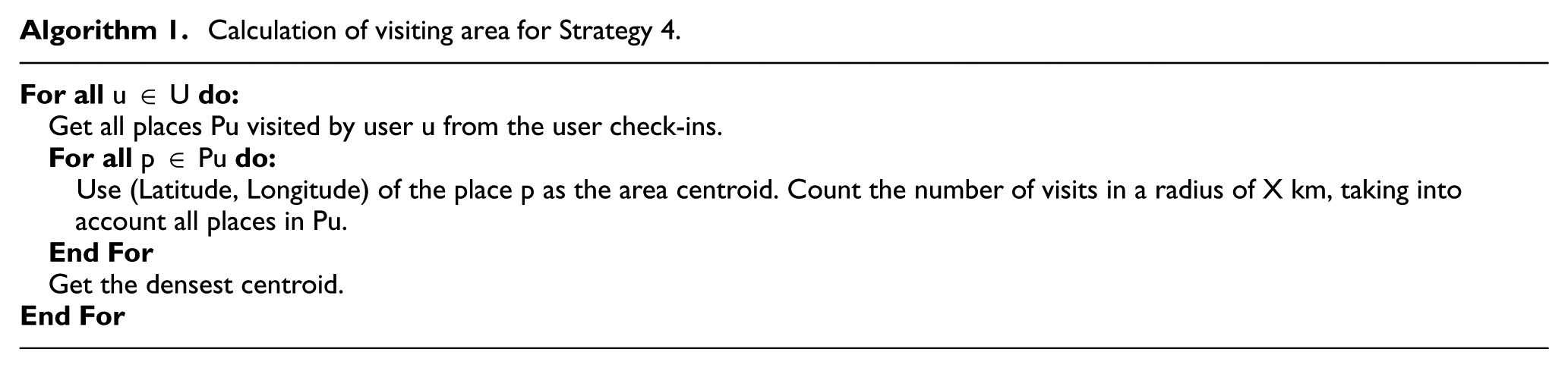
For Strategy 3, the variable ‘Home city’ from the user profiles was considered to group users from New York in counties (e.g. Manhattan, Brooklyn, Queens). We used the service from Google maps³ to obtain more information about the place of residence. New York has 67 counties, but only 57 counties appeared in our dataset, since some counties have very few users. For Strategy 4, two steps were required. First, we obtained the places visited for each user according to the check-ins made and calculated the visiting area considering, which is the geographical zone that contains the biggest number of visited places in a radio of 1 km, according to Algorithm 1. Then, the distance between the areas visited by two users was calculated using the cosine measure regarding their centroids and considering the earth radius of 6378.1 km. To carry out the evaluation, we separated the training and test data using a 70–30 partition. Thus, for each user in the dataset we randomly selected the 30% of his visits (user, POI, preference) for testing and the remaining 70% was used for training.

Algorithm 1.

Calculation of visiting area for Strategy 4.

For all u ∈ U do:
Get all places Pu visited by user u from the user check-ins.
For all p ∈ Pu do:
Use (Latitude, Longitude) of the place p as the area centroid. Count the number of visits in a radius of X km, taking intoaccount all places in Pu.
End For
Get the densest centroid.
End For

4.3. Results obtained

In this section, we present the results obtained when evaluating the different strategies with the two approaches to build the user preferences. First, in section 4.3.1, we present the results obtained with the matrix of user preferences based on visits. Then, in section 4.3.2, we present the results obtained with the user preferences based on the sentiment of tips. Finally, in section 4.3.3, we briefly analyse the results obtained.

4.3.1. Results for preferences based on visits

Figure 3 shows the experimental results obtained for the different strategies considering the matrix based on user visits. In Figure 3(a), it is possible to observe the results considering different levels of friend relationships according to Strategy 1. The Baseline is the traditional CF approach that selects the k most similar users based on the cosine similarity of their preferences exclusively. Considering a single level of relationships, that is, only the direct friends of the target user, the results obtained are considerably worse than the baseline. The results for levels 3, 4 and 5 are similar to the results obtained for the baseline, being slightly better for neighbours of sizes up to 100 users. For relationships of level 2, that is, friends of friends, the results are better than the baseline for small neighbours (up to 50 users) but then become slightly worse.

Figure 3.

Experimental results on the matrix of visits for (a) Strategy 1 (b) Strategy 2 and (c) Strategies 3, 4.

Figure 3(b) shows the results considering the network formed by common visited places defined in Strategy 2. This strategy outperformed the baseline in all its variations. The best performing option was using the direct edges, that is, users that visit the same places than the target user. Exploring further the graph of common visited places, the MAE values grow, even though they are still lower than the baseline.

Figure 3(c) reports the results of the strategies concerning with geo-localisation (Strategies 3 and 4). We can observe that for neighbours up to 100 users the strategy considering the visiting area achieved better results than the baseline. For even smaller neighbours, considering users living in the same state also obtained good results. However, for bigger neighbourhoods, all the strategies considering geographical information behaved very similarly, marginally outperformed by the baseline.

4.3.2. Results for preferences based on tips

Figure 4 shows the results obtained with the proposed strategies and the preference matrix built from tips. In Figure 4(a), we can observe the results obtained with the strategy where friend relations at different levels among users of the system are considered. We can see that, in general, for 30 neighbours or less, all the levels of friendship have lower estimation error with respect to the baseline, that is, the classical CF approach, seeking the k most similar users to target user using the cosine similarity. It is also noted that the relationships of level 1 or direct friends lead to reduced error values than the rest. Relationships of level 2 also achieved better results than the baseline. However, if we continue to explore the social graph up to level 5 and the number of neighbours increases, the error values obtained are similar to the baseline.

Figure 4.

Experimental results on the matrix of tips for (a) Strategy 1 (b) Strategy 2 and (c) Strategies 3, 4.

Figure 4(b) shows the results of the Strategy 2, which represents the network of common visited places among users. We can observe that all the strategies obtained lower prediction errors than the baseline for medium size neighbourhoods. The best results were obtained for relationships of level 1, that is, considering the opinion of users that visited the same places than the target user. When analysing big neighbourhoods and exploring the graph further, the prediction error increases and tends to be similar to the error of the baseline method.

Finally, Figure 4(c) shows the results of the strategies related to the geo-localisation information, that is, Strategies 3 and 4. It is observed that for neighbourhoods up to 100 users, minor errors were obtained when neighbours were selected from the state of New York, followed by neighbours selected from the same county and, finally, with neighbours selected from the same visiting areas.

4.3.3. Analysis

In general terms, the proposed strategies for selecting neighbours based on the different elements available in LBSNs achieve better results than the traditional CF approach. Therefore, the proposed hypotheses could be validated but they sometimes depend on the size of the neighbourhood and on the level of depth up to which we should explore the networks. An additional advantage of the proposed strategies is the number of users involved in the computation of predictions. User-based CF is based on the similarity computations of the target user with every other user in the dataset, for choosing the k most similar ones. In the proposed strategies, this number of users is reduced. Figure 5 shows the average number of comparisons (similarity computation for a pairs of users) necessary to determine the neighbourhood of users evaluated according to each strategy, in decreasing order. The baseline uses all of the 47,240 users. Regarding to strategy 1 (related to ‘H1’), if the friend relationships are used, the number increases as more levels of the network are explored. The best performing option, which was friend-of-a-friend (level 2) involves 10,649 users (22%). However, strategy 2 (related to ‘H2’), the best performing variation using the network of common visited places (level 1), is based in only 19 users. In strategy 3 (related to ‘H3’), better results are obtained when the size of the neighbourhood is less than 100. However, it involves a large number of users: 27,000 (57%) for the state and 11,707 (25%) for the county. Also, in strategy 4 (related to ‘H4’) using the visiting area of users involves 3111 users (6.5%). Naturally, in the case of Strategies 2 and 4, the visiting graph and the visiting area require previous data calculation and their updating with its consequent computational cost. This effort, however, can be done off-line. Strategies 1 and 3, instead, use data accessible from the profiles in the LBSN (friends and residence).

Figure 5.

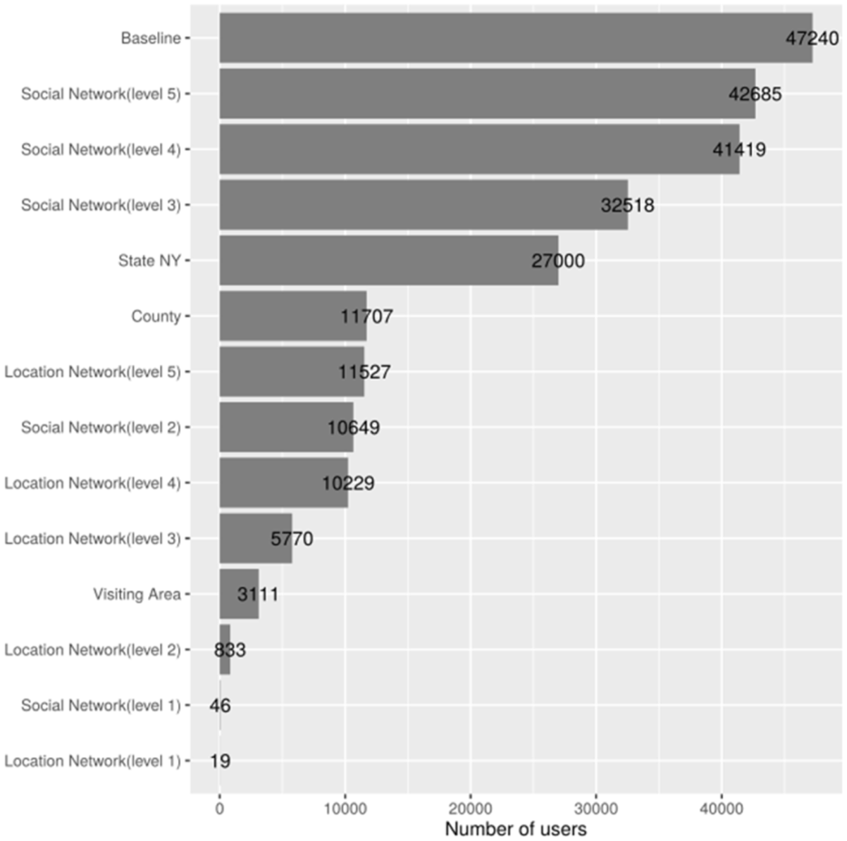
Number of users compared for selecting the neighbourhood.

Figure 6 shows the values for coverage for the different strategies compared with the baseline. The coverage refers to the proportion of user-item pairs for which the system was able to estimate a preference, as shown in equation (4), where $I_{p}$ is the number of user-item pairs for which a preference could be estimated and I is the set of user-item pairs. In our context, a recommendation cannot be made when the user has no neighbours or the neighbours do not rate the item to be recommended. In the user-based CF approaches, the coverage is generally limited because two users can be neighbours if they visited the same places, thus, if a user has few visits it is probable that he will have few neighbours or none. Also, even if a user has neighbours the estimation can only be made if the neighbours visited the place to be recommended

Coverage = \frac{| I_{p} |}{| I |}

(4)

Figure 6.

Coverage for the different selection strategies.

Regarding the results of coverage obtained, it can be observed that as the number of neighbours grows the coverage value is higher. This is because there are more chances to recommend an item when the number of neighbours of a user is high. However, we can observe that the coverage value is different for the different strategies considered, showing that some of them have coverage values that are better than for the baseline. The strategies considering user relationships based on common visits obtained the best results. Regarding strategies based on social or friendship relations, we can observe that the level 1 (only direct friends) got the worst results. Finally, regarding strategies based on geographical information, we can observe that the one based on visiting area obtained better results than the other, with results similar to the baseline, and the ones obtained for the social based approach for levels 3 and 5.

In order to compare the results of the strategies over the different matrices, visits and tips, Table 2 summarises the percentage of improvement of the best performing settings over the baseline (the traditional CF approach) for neighbourhood sizes of 10, 50 and 300 and highlights (italics) in which matrix the strategies achieved their best performance. Note that MAE values are not directly comparable as in each matrix we are predicting different things (what will be the sentiment of a user towards a certain item, in one case, and how many visits can be expected, in the other). In general terms, the strategies reach better levels of improvement when applied to the matrix of tips, except for the location network approach that is using visits for building the graph, which improves the most with a matrix of visits. In Table 2, we can also observe the behaviour of our strategies in relation to the FBCF (another baseline). It can be noted that although FBCF outperforms the baseline in the matrix of tips, its improvements are below the improvements achieved by most of our strategies. In addition, FBCF performed considerably worse on the matrix of visits than on the matrix of tips.

Table 2.

Percentage of improvement of strategies over the baseline for the different matrices.

		FBCF (%)	Social networks (%)	Location networks (%)	Geographical (%)
10	Visit	−7.3	0.8	11.2	6.5
	Tips	6.4	10.9	7.5	7.8
50	Visit	−6.3	1.2	6.6	4.5
	Tips	0.3	4.0	2.0	1.9
300	Visit	−7.9	−0.2	0.9	−1.0
	Tips	2.8	3.2	1.1	−0.2

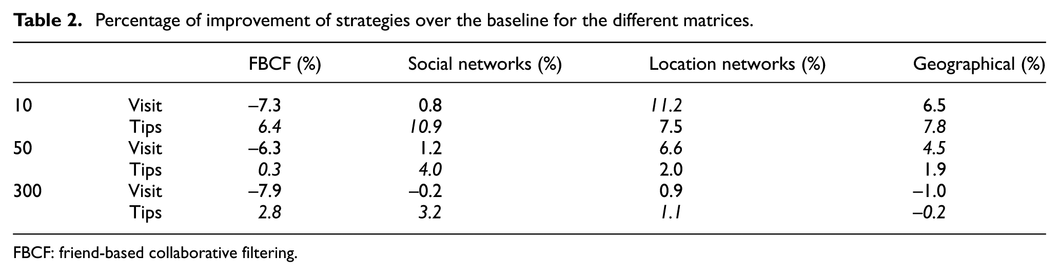
FBCF: friend-based collaborative filtering.

5. Conclusion

POI recommendation is an effective method to assist users in LBSNs. In this article, we have proposed different strategies for selecting neighbours in the context of CF for the recommendation of places of interest (POIs) in LBSNs. Two alternative approaches for obtaining user preferences from LBSNs have been considered in combination with these strategies, the visiting history of users and the sentiment analysis of their comments.

From this study, we can conclude that the different elements available in LBSNs, such as the relationships among users and the geo-localisation of data, allow RSs to select users that are potentially more useful for prediction, particularly when small neighbourhoods are considered (up to 100 users). We studied four strategies, two based on relationships such as friendship and co-located visits and two using geographical information, such as the place where users live and walk around. All of these strategies were capable of improving the baseline, the traditional user-based CF approach. More importantly, the proposed strategies are less computational expensive than the baseline as the prediction of preferences is based on a reduced number of users, those having some kind of relationship (social or geographical) instead of the entire community. The best performing strategy for selecting neighbours was the one that chose users from those that share visited places with the target user, that is, those that visited at least a place that has been visited by the target user. Notably, this strategy not only reduced the error in prediction significantly but also was the one involving the evaluation of fewer users in the prediction step of the CF approach.

These findings can be helpful both to researchers in the RSs area and to developers implementing recommendation strategies in the context of LBSNs, since they can take into account our results to design and provide personalised services considering the information available in LBSNs. Likewise, the findings regarding coverage and computational cost of strategies when exploring a user dataset might have practical implications in the development of recommendation systems in scenarios with scarce resources.

As regards future work, we plan to integrate other elements of LBSNs such as the category a place belongs to, as well as to evaluate functions to weight the selected neighbours for improving prediction. Also, we plan to evaluate different strategies for combining selection and scoring of users (function f in equation (1)), as well as the aggregation of the different information sources which were considered in this work separately. As regards the analysis of tips, we can also extract the opinion of each tip separately instead of considering all the tips about a certain place given by a user together.

Footnotes

Declaration of conflicting interests

The author(s) declared no potential conflicts of interest with respect to the research, authorship and/or publication of this article.

Funding

This work has been partially funded by CONICET, Argentina.

Notes

References

Ricci

Rokach

Shapira

. Introduction to recommender systems handbook. In: Ricci

Rokach

Shapira

et al . (eds) Recommender systems handbook. New York: Springer, 2011, pp. 1–35.

Bao

Zheng

Wilkie

et al . Recommendations in location-based social networks: a survey. Geoinformatica 2015; 19(3): 525–565.

Zafarani

Abbasi

Liu

. Social media mining: an introduction. Cambridge: Cambridge University Press, 2014.

Papadimitriou

Symeonidis

Manolopoulos

. Friendlink: link prediction in social networks via bounded local path traversal. In: Proceedings of the international conference on computational aspects of social networks, Salamanca, 19–21 October 2011, pp. 66–71. New York: IEEE.

Scellato

Noulas

Mascolo

. Exploiting place features in link prediction on location-based social networks. In: Proceedings of the 17th ACM SIGKDD international conference on Knowledge discovery and data mining (KDD ’11), San Diego, CA, 21–24 August 2011, pp. 1046–1054. New York: ACM.

Bellotti

Begole

Chi

et al . Activity-based serendipitous recommendations with the Magitti mobile leisure guide. In: Proceedings of the SIGCHI conference on human factors in computing systems (CHI ’08), Florence, 5–10 April 2008, pp. 1157–1166. New York: ACM.

Zanda

Menasalvas

Eibe

. A social network activity recommender system for ubiquitous devices. In: Proceedings of the 11th international conference on intelligent systems design and applications (ISDA 2011), Cordoba, 22–24 November 2011, pp. 493–497. New York: IEEE.

Lee

Wakamiya

Sumiya

. Discovery of unusual regional social activities using geo-tagged microblogs. World Wide Web 2011; 14(4): 321–349.

Quercia

Lathia

Calabrese

et al . Recommending social events from mobile phone location data. In: Proceedings of the 10th international conference on data mining (ICDM 2010), Sydney, NSW, Australia, 13–17 December 2010, pp. 971–976. New York: IEEE.

10.

Long

Joshi

. A HITS-based POI recommendation algorithm for Location-Based Social Networks. In: Proceedings of the IEEE/ACM international conference on advances in social networks analysis and mining (ASONAM 2013), Niagara Falls, ON, Canada, 25–28 August 2013, pp. 642–647. New York: IEEE.

11.

Ajao

Hong

Liu

. A survey of location inference techniques on Twitter. J Inf Sci 2015; 41(2): 855–864.

12.

Yin

Sun

Cui

et al . LCARS: a location-content-aware recommender system. In: Proceedings of the 19th ACM SIGKDD international conference on knowledge discovery and data mining (KDD ’13), Chicago, IL, 11–14 August 2013, pp. 221–229. New York: ACM.

13.

Wang

Zhao

Nie

et al . Semantic-based location recommendation with multimodal venue semantics. IEEE T Multimedia 2015; 17(3): 409–419.

14.

Park

Hong

Cho

. Location-based recommendation system using Bayesian users preference model in mobile devices. In: Proceedings of the 4th international conference on ubiquitous intelligence and computing (UIC’07), Hong Kong, China, 11–13 July 2007, pp. 1130–1139. New York: ACM.

15.

Lian

Yuan

et al . Sparse Bayesian content-aware collaborative filtering for implicit feedback. In: Proceedings of the twenty-fifth international joint conference on artificial intelligence (IJCAI-16), New York, 9–15 July 2016, pp. 1732–1738. New York: ACM.

16.

Levandoski

Sarwat

Eldawy

et al . LARS: a location-aware recommender system. In: Proceedings of the 28th international conference on data engineering (ICDE ’12), Washington, DC, 1–5 April 2012, pp. 450–461. Washington, DC: IEEE Computer Society.

17.

Zhang

Chow

Zheng

. ORec: an opinion-based point-of-interest recommendation framework. In: Proceedings of the 24th ACM international conference on information and knowledge management (CIKM2015), Melbourne, VIC, Australia, 18–23 October 2015, pp. 1641–1650. New York: ACM.

18.

Chen

et al . MARS: a multi-aspect recommender system for point-of-interest. In: Proceedings of the 31st international conference on data engineering (ICDE 2015), Seoul, South Korea, 13–17 April 2015, pp. 1436–1439. New York: IEEE.

19.

Berjani

Strufe

. A recommendation system for spots in location-based online social networks. In: Proceedings of the 4th workshop on social network systems (SNS ’11), Salzburg, 10–13 April 2011, Article 4. New York: ACM.

20.

Lian

Zhao

Xie

et al . GeoMF: joint geographical modeling and matrix factorization for point-of-interest recommendation. In: Proceedings of the 20th ACM SIGKDD international conference on knowledge discovery and data mining (KDD ’14), New York, 24–27 August 2014, pp. 831–840. New York: ACM.

21.

Huang

Gartner

. Using context-aware collaborative filtering for POI recommendations in mobile guides. In: Proceedings of the 8th international symposium on location-based services (LBS 2011), Vienna, 21–23 November, 2011, pp. 131–147.

22.

Zhou

Huang

. A point-of-interest recommendation method based on user check-in behaviors in online social networks. In: Proceedings of the 4th international conference on computational social networks (CSoNet 2015), Beijing, China, 4–6 August 2015, vol. 9197, pp. 160–171. Cham: Springer.

23.

Yin

Lee

et al . Exploiting geographical influence for collaborative point-of-interest recommendation. In: Proceedings of the 34th international ACM SIGIR conference on research and development in information retrieval (SIGIR ’11), Beijing, China, 24–28 July 2011, pp. 325–334. New York: ACM.

24.

Cheng

Yang

King

et al . Fused matrix factorization with geographical and social influence in location-based social networks. In: Proceedings of the 26th AAAI conference on artificial intelligence (AAAI’12), Toronto, ON, Canada, 22–26 July 2012, pp. 17–23. Palo Alto, CA: AAAI Press.

25.

Nunes

Marinho

. A personalized geographic-based diffusion model for location recommendations in LBSN. In: Proceedings of the 9th Latin American web congress (LA-WEB 2014), Ouro Preto, 22–24 October 2014, pp. 59–67. New York: IEEE.

26.

Gao

Tang

Liu

. gSCorr: modeling geo-social correlations for new check-ins on location-based social networks. In: Proceedings of the 21st ACM international conference on information and knowledge management (CIKM ’12), Maui, HI, 2 November 2012, pp. 1582–1586. New York: ACM.

27.

Tang

Gao

et al . Exploiting local and global social context for recommendation. In: Proceedings of the 23rd international joint conference on artificial intelligence (IJCAI ’13), Beijing, China, 3–9 August 2013, pp. 2712–2718. New York: ACM.

28.

Hong

et al . Point-of-interest recommendations: learning potential check-ins from friends. In: Proceedings of the 22nd ACM SIGKDD international conference on knowledge discovery and data mining (KDD ’16), San Francisco, CA, 13–17 August 2016, pp. 975–984. New York: ACM.

29.

Zhang

Chow

. GeoSoCa: exploiting geographical, social and categorical correlations for point-of-interest recommendations. In: Proceedings of the 38th international ACM SIGIR conference on research and development in information retrieval (SIGIR ’15), Santiago, Chile, 9–13 August 2015, pp. 443–452. New York: ACM.

30.

Fang

Dai

. Power of bosom friends, POI recommendation by learning preference of close friends and similar users. In: Proceedings of the international conference on big data analytics and knowledge discovery (DaWaK 2016), Porto, 5–8 September 2016, pp. 179–192. Cham: Springer.

31.

Zukerman

Albrecht

Nicholson

. Predicting users requests on the WWW. In: Proceedings of the 7th international conference on user modeling (UM’99), Banff, AB, Canada, 20–24 June, 1999, pp. 275–284.

32.

Bellogín

Castells

Cantador

. Neighbor selection and weighting in user-based collaborative filtering: a performance prediction approach. ACM T Web 2014; 8(2): 12.

33.

Yang

Zhang

et al . A sentiment-enhanced personalized location recommendation system. In: Proceedings of the 24th ACM conference on hypertext and social media (HT ’13), Paris, 1–3 May 2013, pp. 119–128. New York: ACM.

34.

Yang

Zhang

et al . Fine-grained preference-aware location search leveraging crowdsourced digital footprints from LBSNs. In: Proceedings of the ACM international joint conference on pervasive and ubiquitous computing (UbiComp ’13), Zurich, 8–12 September 2013, pp. 479–488. New York: ACM.

35.

Chen

Wang

. Recommender systems based on user reviews: the state of the art. User Model User: Adap 2015; 25: 99–154.

36.

Wang

Sun

. Exploiting location significance and user authority for point-of-interest recommendation. In: Advances in knowledge discovery and data mining: 21st Pacific-Asia conference (PAKDD 2017), Jeju, South Korea, 23–26 May 2017. Cham: Springer.

37.

Yuan

Cong

et al . Time-aware point-of-interest recommendation. In: Proceedings of the 36th international ACM SIGIR conference on research and development in information retrieval, Dublin, 28 July–1 August 2013, pp. 363–372. New York: ACM.

38.

Liu

Wei

Sun

et al . Exploiting geographical neighborhood characteristics for location recommendation. In: Proceedings of the 23rd ACM international conference on information and knowledge management, Shanghai, China, 3–7 November 2014, pp. 739–748. New York: ACM.

39.

Gao

Tang

et al . Exploring temporal effects for location recommendation on location-based social networks. In: Proceedings of the 7th ACM conference on recommender systems, Hong Kong, China, 12–16 October 2013, pp. 93–100. New York: ACM.

40.

Liu

Zhang

. A survey of opinion mining and sentiment analysis (ed Aggarwal

Zhai

). Boston, MA: Springer, 2012, pp. 415–463.

41.

Bao

Zheng

Mokbel

. Location-based and preference-aware recommendation using sparse geo-social networking data. In: Proceedings of the 20th international conference on advances in geographic information systems (SIGSPATIAL ’12), Redondo Beach, CA, 6–9 November 2012, pp. 199–208. New York: ACM.