
Abstract
This study presents a solution to a problem commonly known as link prediction problem. Link prediction problem interests in predicting the possibility of appearing a connection between two nodes of a network, while there is no connection between these nodes in the present state of the network. Finding a solution to link prediction problem attracts variety of computer science fields such as data mining and machine learning. This attraction is due to its importance for many applications such as social networks, bioinformatics and co-authorship networks. Towards solving this problem, Evolutionary Link Prediction (EVO-LP) framework is proposed, presented, analysed and tested. EVO-LP is a framework that includes dataset preprocessing approach and a meta-heuristic algorithm based on clustering for prediction. EVO-LP is divided into preprocessing stage and link prediction stage. Feature extraction, data under-sampling and feature selection are utilised in the preprocessing stage, while in the prediction stage, a meta-heuristic algorithm based on clustering is used as an optimiser. Experimental results on a number of real networks show that EVO-LP improves the prediction quality with low time complexity.
Keywords
1. Introduction
This study introduces an approach to optimise a solution for link prediction problem by utilising the advantageous features of clustering and meta-heuristic algorithms, such as Moth-Flame Optimisation algorithm (MFO), Genetic Algorithm (GA), Particle Swarm Optimisation (PSO), Whale Optimisation Algorithm (WOA) and Differential Evolution (DE). The target is to get a potential solution to the problem of predicting the possibility of a future connection between two nodes of a network, knowing that there is no connection between these nodes in the present state of the network.
Generally, graphs provide a natural abstraction to represent interactions between different entities in a network [1]. A real or synthetic network in the world can be represented as a graph of nodes and edges. As in social network, users are represented as nodes, while the interactions between these users whether are associations, collaborations or influences are presented as edges between these nodes [2]. For instance, if there is a snapshot of a social network at time t0, link prediction looks for predicting the edges that will be added to the network during the interval from time t0 to a given future time t accurately [2]. So, the link prediction problem is related to the problem of inferring missing links from an observed network [2].
Importance of link prediction can be found in its wide variety of applications. Graphs could be represented as social networks, transportation networks or disease networks [1]. Link prediction can specifically be applied on these networks to analyse and solve interesting problems like predicting outbreak of a disease, controlling privacy in networks, detecting spam emails, suggesting alternative routes for possible navigation based on the current traffic patterns and so on [1].
More formally, the link prediction task can be formulated as follows [2]. An un-weighted and undirected graph G = (V, E) represents a topological structure of a network, such as social networks, where V is the set of nodes in G, and E is the set of existed edges in G. In this G, each edge e = (u, v) ∈ E and nodes u, v ∈ V represents an interaction between u and v that took place at a particular time t(e). For two time instances, t and t′, where t′ > t, let G[t, t′] denotes a sub-graph of G consisting of all edges with timestamps between t and t′, and let t0,
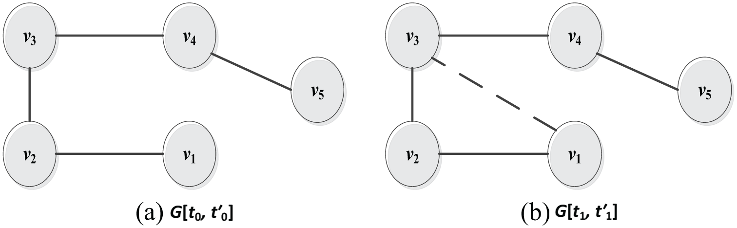
Different snapshots of the network G at two time intervals. (a) A snapshot of a network at time [t0,
There are three types of link prediction problems [3]. (1) Only adding edges to the existing network, (2) only removing edges from the existing structure and (3) both, adding and removing edges at the same time. This study focuses on the first type of link prediction, only adding edges to the existing network.
To understand why link prediction is considered as a problem, suppose a network G’(V, E’) be an undirected, and un-weighted graph that represents the observed network. Let the complete graph denoted by G(V, E), then G’ is a sub-graph of G and the set of missing edges is E – E’. For an edge e not belonging to E’, the job is to estimate the likelihood that e ∈ (E – E’).
Consequently, there are (|V|*|V− 1|/2) - |E’| possible missing edges to predict from the existing observed network G’. If G’ is a dense graph, then |E’| will be close to ((|V|*|V− 1|/2) − b), where b is some constant between 1 and |V|. Thus, there is a constant number of missing edges to choose from, c, and O(1/c) probability of choosing these missing edges correctly at random. If G’ is a sparse graph, then |E’| will be close to (|V| − 1). Thus, we have a ((|V|*|V− 1|/2) edges to choose from, and O(2/(|V|*|V− 1|)) probability of choosing correctly at random. This is summarised in Table 1 and presented in Figure 2.
A comparison between dense and sparse graph based on the probability of choosing at random.

V is a set of nodes, E is a set of edges, b is a constant between 1 and |V| and c is number of edges to choose from.
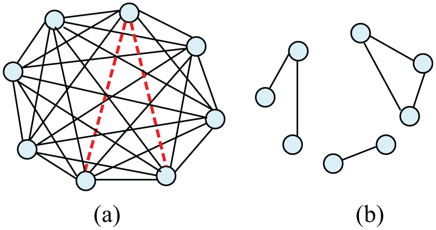
Predicting the correct edge in a sparse graph versus a dense graph. (a) A dense graph with two edges, out of 28, to predict from (red dashed lines) and (b) a sparse graph with 22 edges to predict from.
Unfortunately, there are many networks, such as social networks, that are sparse. So, there is a need to find a way to narrow this probability down and make link prediction a more feasible problem. In this case, the need for meta-heuristic algorithms actually rises to guarantee finding the optimal prediction quality in a reasonable time.
The structure of this study is as follow: Section 2 presents the related works of link prediction. Section 3 describes the methodology of EVO-LP framework with illustrated example. Section 4 is about the complexity analysis of EVO-LP. Section 5 presents the data setup. Section 6 shows the experimental results and their discussions. Finally, conclusions and future work are in Section 7.
2. Related works
Due to the importance of link prediction problem in network science and its applications in different field, various approaches were proposed to provide a potential solution for prediction. This study will focus mainly on approaches used static, undirected and un-weighted networks type.
Liben-Nowell and Kleinberg [2] formalised the question ‘Given a snapshot of a social network, can we infer which new interactions among its members are likely to occur in the near future?’ as the link prediction problem. They developed approaches to link prediction based on measures for analysing the ‘proximity’ of nodes in a network. In their work, they focused mainly on static link prediction problem especially for social networks [2].
Their proposed methods are adapted from techniques used in graph theory and social network analysis. All these methods assign a connection weight score(x, y) to pairs of nodes (x, y), based on the input graph G, and then produce a ranked list in decreasing order of score(x, y). This score represents the local similarity measure between the nodes x and y. Some of these methods are based on node neighbourhoods, such as Common Neighbours (CN), Jaccard’s Coefficient (JC) [4], Adamic/Adar (AA) and Preferential Attachment (PA). Others are based on the ensemble of all paths, such as Katz, Hitting time, PageRank and SimRank [2]. In their work, five datasets from which co-authorship networks were constructed are used: astro-ph (astrophysics), cond-mat (condensed matter), gr-qc (general relativity and quantum cosmology), hep-ph (high energy physics–phenomenology) and hep-th (high energy physics–theory). To more meaningfully represent predictor quality, they used a random predictor as baseline. Each predictor’s performance on each dataset is measured in terms of the factor improvement over this random predictor. As a result, some of the very simple measures perform surprisingly well, including CN and the AA measure [2].
Li et al. [5] proposed a similarity index for link prediction. Unlike most of the similarity-based algorithms which only focus on the roles of paths connecting two nodes but ignore the influences of two nodes themselves, they considered the roles of paths to end nodes in the network and the roles of end nodes themselves. Their proposed method not only distinguishes the roles of different paths but also integrates the roles of the end nodes. Consequently, their method obtained better performance on accuracy.
Lichtenwalter et al. [6] presented an effective flow-based predicting algorithm called PropFlow. PropFlow is unsupervised and a global similarity measure based on information flow. It represents the amount of information that flows from the source to the destination node across different paths. The higher the information gathered, the larger the similarity value between source and destination node. In their work, they extracted features such as in-degree, out-degree, PropFlow, Katz, CN and shortest path from two different datasets called cond-mat and phone. Then, they applied two different ensemble methods: bagging and random forests. The performance is measured based on the value of area under receiver operating characteristic (ROC) curve. The general framework they proposed achieves major improvements over existing methods. They did not make any feature selection methods to choose which feature set will be the suitable set. However, they use only features that are mentioned in Lichtenwalter et al. [6] for generality, but any other available features, including measures of reciprocity or node attributes, could be used.
Many other works take the advantages of supervised machine learning methods or algorithms for link prediction problem. Al Hasan et al. [7] studied link prediction as a supervised learning task. They identified a short list of features for link prediction in the co-authorship domain (BIOBASE, and DBLP datasets). These features include Proximity Features, Aggregated Features and topological features. For BIOBASE dataset, nine features are used, and for the DBLP dataset only four features are used. The algorithms that they used are SVM, Decision Tree, Multilayer Perceptron, K-Nearest Neighbours, Naive Bayes, RBF Network and Bagging. They evaluate the result using accuracy, precision, recall, F-value and squared error. They showed that a small subset of features always plays a significant role in link prediction.
Kashima et al. [8] presented an efficient incremental supervised learning algorithm based on a probabilistic model. This model used topological features of the network structure for predicting links between the nodes.
Raymond and Kashima [9] proposed fast and scalable algorithms compared with Kashima et al. [8] for link propagation by introducing efficient procedures to solve large linear equations that appear in the method.
Cukierski et al. [10] incorporated 94 distinct graph features, as in Srinivas and Mitra [1], used as input for classification with Random Forests on flickr graph and using area under the curve (AUC) as performance metrics. One of their conclusions is, it is common practice to abstract social networks as graphs and develops highly general methods for characterising them.
Feng et al. [11] tried to understand how the network structure affects the performance of link prediction methods in the view of clustering. Their experiments on both synthetic and real-world networks show that as the clustering grows, the accuracy of these methods could be improved remarkably, while for the sparse and weakly clustered network, they perform poorly.
Guimerà and Sales-Pardo [12] supposed the stochastic block models empirically grounded because they capture fundamental properties of complex networks. The six similarity-based measures include CN, AA index, Resource Allocation (RA) index, Katz index, rooted PageRank and superposed Random walk. They used Political blogs, NetScience and Power grid as real-world datasets for testing. Precision and AUC are the performance measures for their results.
Thi and Hoang [13] concentrated on the extraction of more features from user to improve the quality of predicted links. They proposed a measure calculating the similarity of individuals. The measure considers not only network topology but also the personal features. They performed experiments on ArXiv HEP-Th. This dataset is a collection of abstract paper in theoretic high energy physics in 12 years (1992–2003), which includes 29,555 publications. Performance of prediction is evaluated on AUC score. The higher similarity score, the more ability a new link appears.
Feyessa et al. [14] used a backpropagation neural network to predict existence or emergence of a link between pairs of nodes using node pair properties such as reciprocity, transitivity and shared neighbours. A limited network visibility by individual nodes is assumed; hence, the size of the node pair feature vector varies with the given visibility range. Their approach is tested on a large social object centred trust network where visibility is limited to two hops, and 828 accurate predictions out of 1000 pair of nodes are achieved. The performance of link prediction approaches is evaluated by constructing a ROC curve as most classification algorithms.
Furthermore, nature-inspired-based approaches are used to resolve the link prediction problem. These techniques mostly include meta-heuristic optimisation algorithms. These algorithms can be defined as a higher level procedure that intended to discover, generate or choose a heuristic that will be responsible to offer a proper good solution to an optimisation problem [15].
There are number of works that take the advantages of evolutionary algorithms for link prediction such as in previous works [16–18]. Chen and Chen [16] proposed a link prediction algorithm using the well-known ant colony optimisation algorithm (ACO). By exploiting the swarm intelligence, the algorithm employs simulated ants to pass through on a reasonable graph. The ant pheromone and heuristic information are assigned in the edges of the reasonable graph. The pheromone on each link is used as the final score of the similarity between the nodes. Experimental results on a number of real networks show that using ACO algorithm improves the prediction precision while maintains low time complexity in comparison with other traditional link prediction approaches such as Katz, CN and Jaccard.
Bliss et al. [17] provided an approach to predicting future links by applying the Covariance Matrix Adaptation Evolution Strategy (CMA-ES) to optimise weights which are used in a linear combination of 16 neighbourhood and node similarity indices. They used topological similarity indices. For node similarity, they calculated four indices: Twitter Id similarity, tweet count similarity, word similarity and happiness similarity. One of the most interesting parts of this work is the detection of similarity indices which develops to have large, positive weights in their link predictors. Perhaps the most remarkable similarity index for which this is the case is the RA index.
For most sparse networks, link prediction becomes a difficult task. The difficulty comes from the question: How to get high prediction accuracy while maintaining low execution time? Therefore, this study proposes a framework that includes dataset preprocessing approach and a meta-heuristic algorithm based on clustering for prediction. Meta-heuristic (or evolutionary) algorithms are GA, MFO, PSO, WOA and DE. This framework is called ‘EVO-LP’ for Evolutionary–Link Prediction and will be explained in the next section.
3. Methodology of EVO-LP
This section describes the methodology of the proposed EVO-LP framework. EVO-LP is a meta-heuristic framework based on preprocessed datasets and data clustering for Link prediction. This framework is divided into two stages. First, a preprocessed stage is applied on the original dataset for a particular network. This dataset consists of a list of the network’s existing edges. Second, link prediction stage is handled by a meta-heuristic algorithm that is mapped as a classifier using data clustering to predict links and evaluate the prediction results. Note that this framework considers only the prediction of link appearance.
Example 1. To illustrate ‘EVO-LP’ stages, an example of applying these stages on a small and simple network N of six nodes and five existed edges, as in Figure 3(a), is given. This network has the corresponding edge list (pair of nodes). Edge list, as in Figure 3(b), represents an example of a raw dataset used as an input for the preprocessing stage.

An example of a network N: (a) a network of six nodes and five edges and (b) corresponding existing edge instance list of the graph in (a).
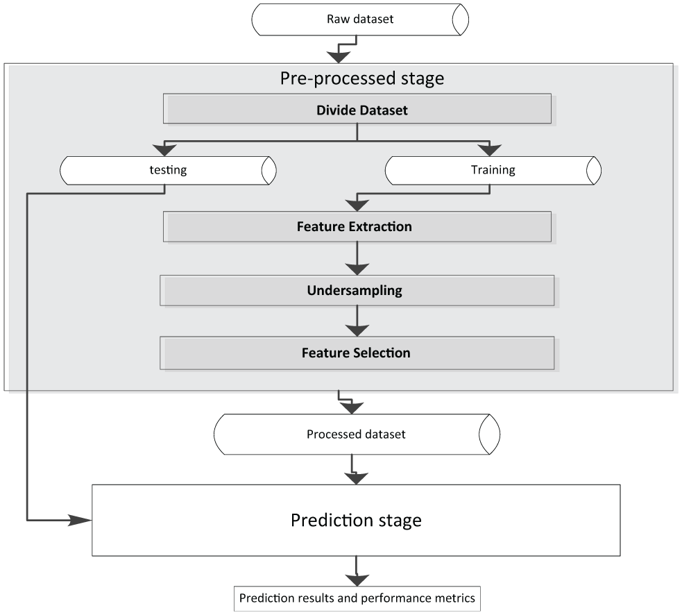
3.1. Preprocessed stage
This stage includes four steps: data division into training and testing sets, feature extraction, under-sampling data instances and feature selection. Preprocessed stage of EVO-LP is modelled in detail in Figure 4.
The details of EVO-LP preprocessed stage.
3.1.1. Data division into training and testing sets
Link prediction is a time-related activity; therefore, time-stamped dataset should be used [3]. To achieve that, the raw dataset should be separated into two sets: training set which represents the current state of the network for time stamp [t, t1], and testing set for the network’s future state for the time stamp [t1, t2], where t, t1 and t2 are different time instances and t < t1 < t2. Consequently, given a network graph G(V, E) where V is the set of vertices and E is the set of existed edges in graph G. Then,
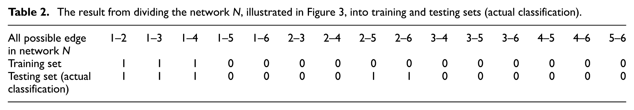
Example 1 (continue). To apply this step, network N which is depicted in Figure 3 can be divided into training and testing sets of edges. For instance, both existed edges 2–5 and 2–6 are selected for testing and the remaining ones are for training, as shown in Table 2.
The result from dividing the network N, illustrated in Figure 3, into training and testing sets (actual classification).
3.1.2. Feature extraction
Feature is defined as a function of the basic measurement variables or attributes that specify some quantifiable property of an object and is useful for classification and/or pattern recognition [19]. Feature extraction is the process to represent raw data in a reduced form to facilitate decision making such as pattern detection, classification, prediction or recognition [19]. Obtaining a good data representation is a very domain-specific task and it is related to the available measurements.
Similarity measures such as CN [2], AA [20], JC [4], PA [21], RA [22], Graph Distance (GD) [2] and PropFlow [6] are considered as features for each edge instance in the training dataset. These measurements could be considered as the topological features for the underlying network. As in Yu et al. [23], the topological features of networks may contribute more to improving performance than other type of features such as node features. Throughout this section, the symbols x, y denote nodes, N denotes number of nodes in the network. Γ(x) and Γ(y) denote the neighbour sets of these nodes and k is the average degree.
CN method assumes that if there are two nodes with many CN, they will be connected in the future. CN can be calculated based on formula (1) [2]

In AA method, the CN of a pair of nodes with few neighbours contributes more to the AA score value than this with large number of relationships. AA can be calculated based on formula (2) [2]

The JC is a statistic measure used for comparing similarity of sample sets. This method is based on CN method and is computed using formula (3) [2]

PA method will calculate similarity score for each pair of nodes within the network rather than only the neighbour of nodes and is computed using formula (4) [2]

In RA, the similarity between the nodes x and y can be defined as the amount of resource y received from x, which is computed using formula (5) [22]

More details about similarity measures such as probFlow and GD can be found in previous works [2, 6, 22]. All these seven measurements are calculated for each edge instance of the training dataset, either it is existed or not. As a result, each edge instance has its own values of the corresponding similarity measures. The result is a new dataset that consists of number of rows and columns. Each row represents an edge instance, while each column represents the computed feature’s scores.
There is an important and additional step after feature extraction, which is called Weighting scores. In order to increase the prediction quality, either in feature selection process or in prediction process, it is better to give the existed edges class a weight to facilitate the differentiation and reduce the overlapping between the corresponding two classes.
Example 1 (continue). As a sample result, a dataset resulted from applying feature extraction process on the training dataset of Network N is presented in Table 3. F represents a set of features. F = {Fi, where i = 1, …, m}, where m is the number of features. The entries in the table are S = {score ij , where i = 1, …, n, and j = 1, …, m}, where n is number of edge instance.
A sample dataset resulted from applying feature extraction process on the training dataset of Network N.

3.1.3. Under-sampling the majority class
In order to process the dataset for prediction, the dataset should be balanced to get suitable values for quality metrics [24–26]. If there is a dataset that contains two classes of instances, one of them is major, while other is minor, then this dataset should be adjusted. This adjustment is made to achieve balancing and ensure fair distribution for both classes. This balancing can be achieved by under-sampling the majority class or over-sampling the minority class in the particular dataset.
Oversampling randomly duplicates the minority class samples, while under-sampling randomly discards the majority class samples in order to modify the class distribution [27]. Because of the sparse nature of most of the social networks, the number of non-existed edges is very large in comparison with existed edges. Therefore, the resulted dataset is imbalanced. To solve the imbalance in the dataset, some instances of the major class should be discarded, and then both classes have the same number of instances.
Solving imbalance in the dataset is a necessary step for both feature selection and link prediction processes. When the dataset is balanced, the selected subset of features through feature selection will be more reliable, and both specificity and sensitivity of dataset’s classes in the link prediction stage will be improved.
3.1.4. Feature selection
Bellman [28] referred to a problem which is called ‘curse of dimensionality’. Curse of dimensionality can rise because the amount of data required to provide a reliable analysis grows exponentially with the dimensionality of the data [29]. A possible solution to this problem is feature selection. Feature selection searches for a projection of the data onto a subset of features which maintains the information as much as possible [29]. Also, feature selection helps to avoid over-fitting the data in order to make further analysis possible [29].
Feature selection works by removing redundant and irrelevant features and selecting only the most significant according to some criterion such as high prediction quality [23]. There are many of feature selection algorithms such as in Sheydaei et al. [30]. Commonly, feature selection algorithms are separated into three categories [29, 31, 32]: (1) the filters which extract features from the data without any learning involved, (2) the wrappers that use learning techniques to evaluate which features are useful and (iii) the embedded techniques which combine the feature selection step and the classifier construction.
In this study, the filter method is used besides GA which is utilised to optimise feature selection quality results measured by accuracy. The GA [33, 34] can be used as a filter to find the better subset of features [35, 36] wherein the chromosome bits represent whether the feature is included or not. Figure 5 shows an example for this chromosome design. The parameters and operators of the GA can be modified within the general idea of an evolutionary algorithm to suit the data to get the best performance [36].

The chromosome design used for feature selection: 1 = for remaining features, and 0 = for filtered out features, where F={Fi, where i = 1, …, n}.
The dataset will be filtered out by deleting features’ column labelled by 0 in the particular chromosome. Then a learning model will be built based on the neural network for this filtered dataset. The result from this model is the predicted classification. By comparing the actual classification with predicted one, the accuracy can be computed. The objective function computes the accuracy as a feature selection performance measurement [36].
As a result, each dataset will have its own subset of features, and then, they will be ready, as inputs, for the next step, prediction stage.
3.2. Link prediction stage
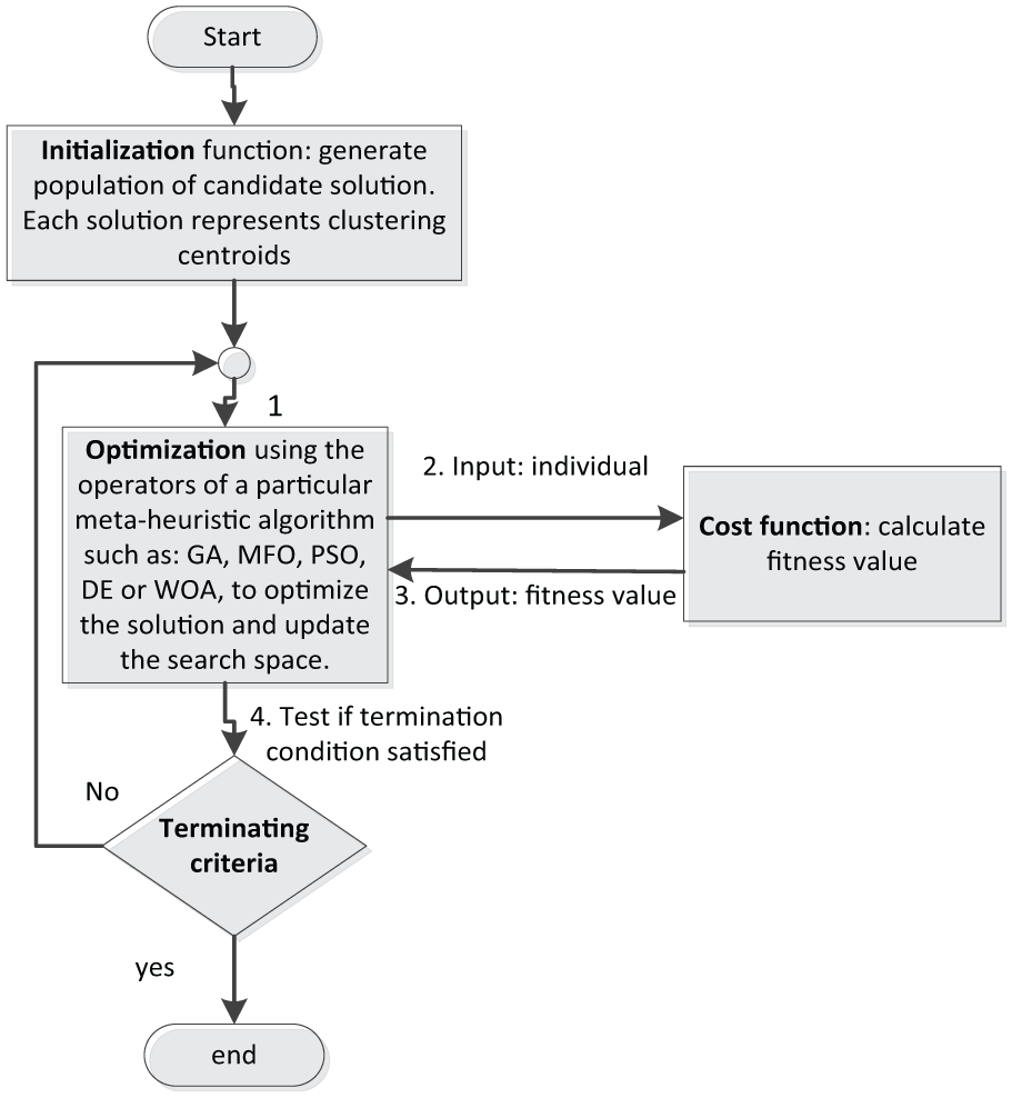
Link prediction stage is the main process in this study. Prediction process is made through clustering the dataset instances into two separated classes; existed or non-existed edges, and optimised through utilising a meta-heuristic algorithm. To build a general framework for link prediction based on meta-heuristic algorithms, link prediction stage should be divided mainly into three functions. These functions are initialisation, optimisation and cost function. Figure 6 shows an overview for the link prediction stage.
EVO-LP’s prediction stage.
3.2.1. Initialisation function
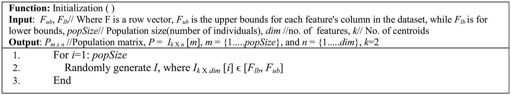
The initialisation function focuses on generating number of specified individuals to build a population. These individuals should be designed in precise and suitable way to support the objective of clustering. Based on clustering, the single individual should represent the centroids. Centroids can be considered as the candidate solution that the instances can be classified based on it, and since there are two possible clusters in this study, there are two centroids to be generated randomly for each individual.
As in Figure 7, each individual is composed of two rows; each row represents a distinct centroid. Each centroid contains number of columns equal to the number of dataset features. The values of each centroid are generated randomly but within the range of upper bound and lower bound for each feature. Figure 8 shows the pseudo-code of the initialisation function.
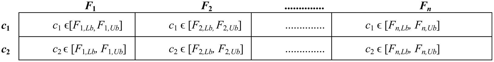
The design of individual I, each I consists of two centroids, c1 and c2, of features F. Each value in the cells should be within the interval of the lower bound (Fi,Lb) and upper bound (Fi,Ub) of the specified feature Fi, where i = 1, 2, …, n.
EVO-LP initialisation function.
3.2.2. Optimisation
In this study, the misclassification rate of prediction should be minimised to obtain more accurate prediction result. So, we need a meta-heuristic algorithm to optimise this value of misclassification. As known, optimisation can be by maximising or minimising the fitness value obtained so far from meta-heuristic iterations.
Commonly, most meta-heuristic algorithms have specified number of iterations. Their termination depends on some criteria or based on the maximum number of iterations. During these iterations, each generation of population, generated by the initialisation function, is updated through exploration and exploitation of the search space. As in Crepinsek et al. [37], ‘Exploration is the process of visiting entirely new regions of a search space, while exploitation is the process of visiting those regions of a search space within the neighbourhood of previously visited points’. With addressing these two processes in meta-heuristic algorithm, the best solution will be closer to find soon.
This study deploys number of meta-heuristic algorithms for link prediction and conducts a comparison between them. These algorithms are as follows: MFO [38], and its modified versions MFO2 and MFO3 [39], WOA [40], PSO [41], GA [42] and DE [43].
MFO, as defined in Mirjalili [38], is a novel nature-inspired meta-heuristic and optimisation paradigm. MFO optimiser is inspired from the navigation methods of moths in nature. The first is called transverse orientation. In this navigation, a moth moves by trying to keep the same angle with regard to the light resource (as known that moths are attracted by light resources). Given that the light resource is distant from the moth, keeping the same angle with respect to the light guarantees moth flying in a straight line. In addition to keep moving in a straight line, moth usually flies spirally around the region of the light, which is considered as the second. Therefore, moth in the long run will converge on its way to the light. Mirjalili [38] utilised these navigation methods, transverse and spiral navigation, and developed the MFO. A conceptual model of these two navigation methods is illustrated in Figure 9.
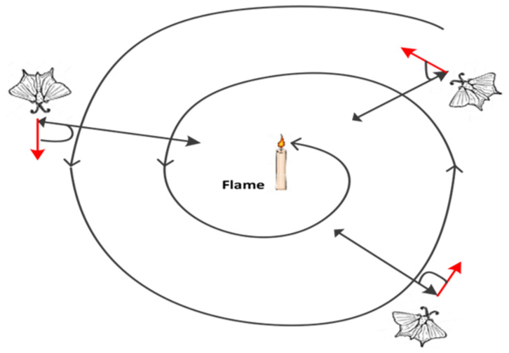
The transverse in a straight line (the red arrow) and the spiral movement of a moth.
The general framework of MFO is as follows: First, in the initialisation stage, MFO generates a random population of moths, and corresponding fitness values. Second, the iteration stage, where the main function is executed and the moths move around the search space. Final stage returns true if the termination criterion is satisfied and false if the termination criterion is not satisfied.
In MFO algorithm [38], a logarithmic spiral is selected as the main update method of moths. This spiral movement is the main component of the MFO because it dictates how the moths update their positions around flames. The spiral movement allows a moth to fly around a flame and not necessarily in the space between them. Therefore, the exploration and exploitation of the search space can be reliable. Logarithmic spiral is defined as in formula (6) [38]

where D indicates the distance of the ith moth from the jth flame, b is a constant for defining the shape of the logarithmic spiral and t is a random number in [−1, 1]. D is calculated as in formula (7)

where M(i, j) indicates the jth position for the ith moth, F(i, j) indicates the jth position for the ith flame and D indicates the distance of the ith moth from the jth flame.
Soliman et al. [39] proposed new versions of MFO, which are called MFO2 and MFO3. They used them to select optimal feature subset for the classification purposes. Instead of using the logarithmic spiral formula as in original MFO, they used the hyperbolic (reciprocal) spiral as in formula (8a) to produce MFO2, and the Archimedean spiral as in formula (8b) to produce MFO3


In addition, Sayedali and Anderew [40] proposed the WOA, which is a recent meta-heuristic optimisation algorithm, which mimic the social activities of whales. The algorithm is inspired from the hunting mechanism of the humpback whales.
PSO, as proposed by Kennedy and Eberhart [41], is a population-based stochastic optimisation technique, inspired by social behaviour of bird flocking or fish schooling, while GA [42] is a meta-heuristic inspired by the process of natural selection that belongs to the larger class of evolutionary algorithms. GAs are commonly used to generate high-quality solutions to optimisation and search problems by relying on bio-inspired operators such as mutation, crossover and selection.
DE [43] is a method that optimises a problem by iteratively trying to improve a candidate solution with regard to a given measure of quality. The principal difference between GA and DE is that GA relies on crossover, while DE strategies use mutation as the primary search mechanism. More details about MFO, MFO2, MFO3, WOA, PSO, GA and DE can be found in previous works [38–43], respectively.
For each of these meta-heuristic algorithms, the main loop that represents the iterations loop and contains their main processes is used to optimise the link prediction results. Figure 10 shows the pseudo-code of MFO main function as an example for the optimisation stage.
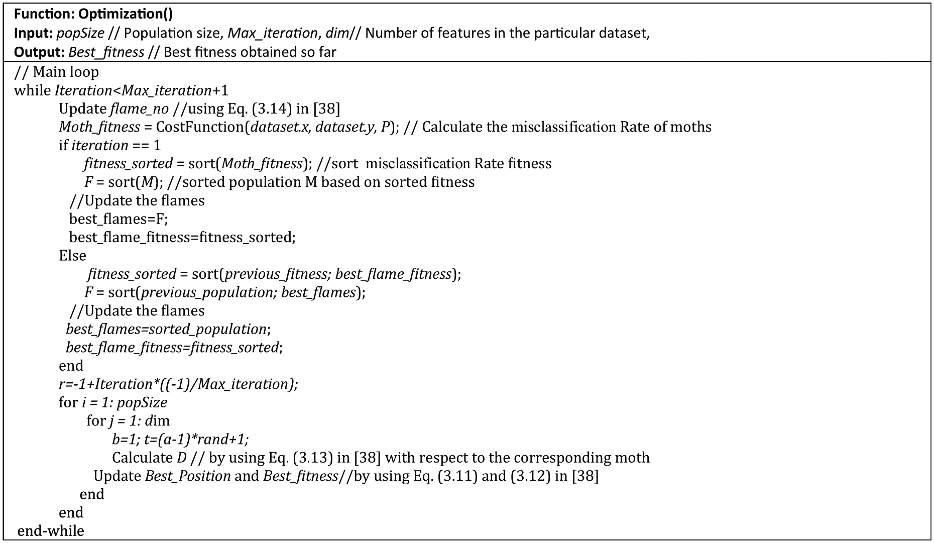
The main steps of MFO algorithm [38].
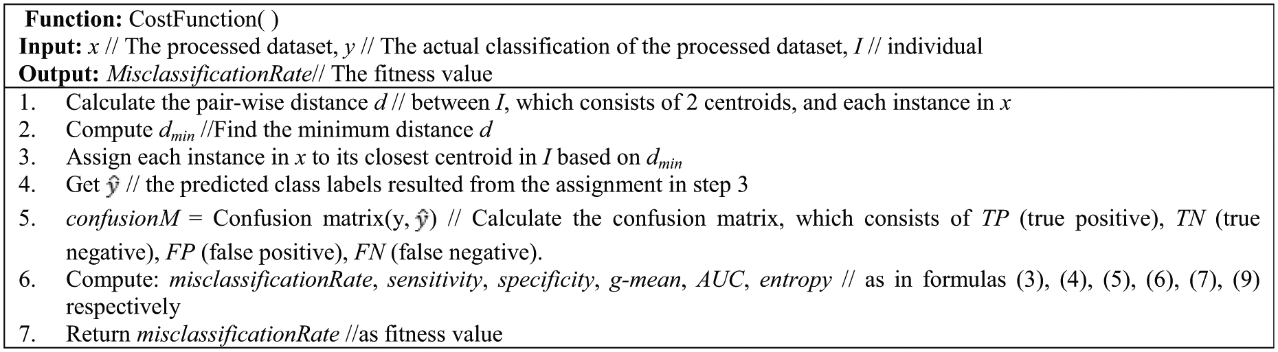
3.2.3. Cost function
The main objective of data clustering is to classify the most similar instances or objects into a same group. Each instance in the dataset is defined by a set of features. To determine similar instances, a similarity measure between them is required [44]. There are many similarity measures used in the literature. This study uses Euclidean distance to calculate the similarity between the instances and the suggested centroids. Euclidean distance is defined as in formula (9). Note that the terms instance and object can be used interchangeably.

Where o is for instance, m is the number of features and oip is the value of the feature number p of the instance number i, ojp is the value of the feature number p of the instance number j.
Each individual of the population generated in the initialisation function is represented as centroids. There will be two centroids, because there are two classes of edges, existed and non-existed edges. Euclidean distance is used to calculate the distance between each instance in the dataset and the specified centroids (individual). According to Euclidean distance, each instance belongs to a specific centroid, when its distance to this centroid is lesser than that for other centroid.
The result of a clustering should be evaluated. This is done by using validity indexes [44]. They are classified into internal and external one [44, 45]. This study uses sum of squares error (SSE), which is an internal validity index. The SSE is a prototype-based cohesion measure where the squared Euclidean distance is used. SSE is defined by formula (10) [44]
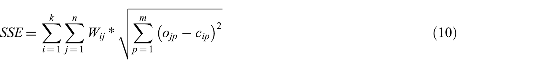
where Wij = 1 if the instance is in the cluster and 0 otherwise, k is the number of clusters, n is the number of instances, m is the number of features and cip is the value of the feature number p of the centroid of the cluster number i (ci) [44].
Each candidate solution has its own SSE value. Calculating SSE helps in classifying instances into their related classes, the resulted classification represents the predicted result. To ensure that this predicted result is validated and reliable, the misclassification rate of its related solution should be calculated. The misclassification rate is an external validity index for the solution and defined by formula (11) [44]

We use misclassification rate in this study because SSE value is not enough to identify the best solution obtained so far. We can have a solution that has the minimum value of SSE but with high misclassification rate. So, after computing SSE for each solution, misclassification rate is required to specify the most validated solution among other solutions. After that, the best solution obtained so far is examined for performance using the following metrics: sensitivity or recall, AUC, G-mean (geometric mean), entropy and the execution time.
To compute the values of these measurements, confusion matrix is required. As in Liu [46], ‘It is convenient to introduce these measures using a confusion matrix, see Table 4. A confusion matrix contains information about actual and predicted results given by a classifier’.
Confusion matrix of a classifier [46].
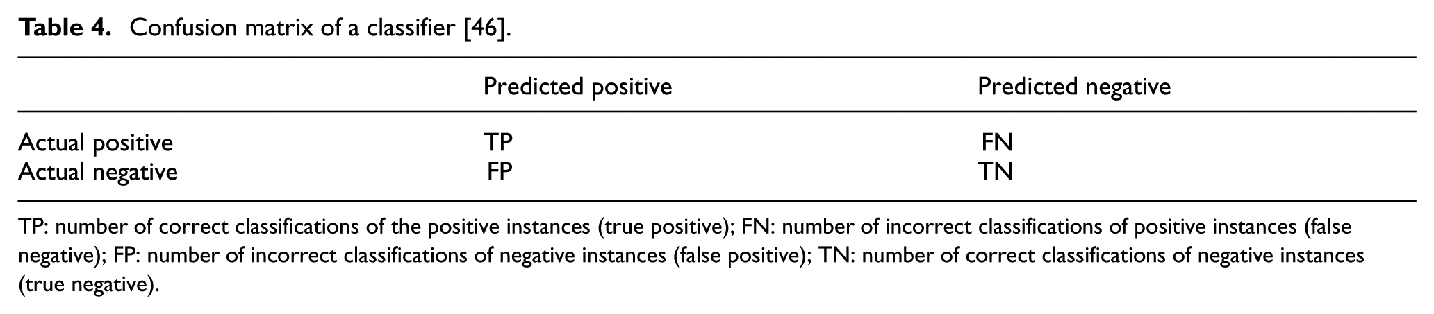
TP: number of correct classifications of the positive instances (true positive); FN: number of incorrect classifications of positive instances (false negative); FP: number of incorrect classifications of negative instances (false positive); TN: number of correct classifications of negative instances (true negative).
Based on the confusion matrix, the recall or sensitivity of the positive class (existed edges in this study) is defined as in formula (12) [46]. Recall measures how precise and how complete the classification is on the positive class. In other words, recall is the number of correctly classified positive examples divided by the total number of actual positive examples in the test set [46]

On the contrary, specificity of the negative class (non-existed edges in this study) is the number of correctly classified negative examples in the test set. Specificity measures how precise and complete the classification is on the negative class. Specificity is defined as in formula (13) [46]

Because the social networks are sparse in their nature, the number of instances in the negative class is much larger than that for positive class. G-mean measures the balanced performance of a learning algorithm between positive and negative classes [47]. G-mean is defined in formula (14) [47]. In this formula, recall represents the accuracy of positive class, while specificity represents negative accuracy. Greater G-mean means better prediction results

A ROC curve is a plot of the true positive rate (TPR) against the false positive rate (FPR) [48]. It is also commonly used to evaluate classification results on the positive class in two-class classification problems. The classifier needs to rank the test cases according to their likelihoods of belonging to the positive class with the most likely positive case ranked at the top [46, 48]. The TPR represents recall, while FPR is defined as in formula (16) [46]. Accuracy is measured by the area under ROC curve or AUC as abbreviation. Greater AUC means better prediction model. AUC could be computed using formula (15)


In addition, entropy is considered as performance measure. Entropy is an external validation measure [49]. The lower entropy means better clustering. The greater entropy means that the clustering is not good. The quantity of disorder is found by using entropy. So, it is expected that every cluster should have low entropy to maintain the quality of clustering results [49]. Entropy is defined as in formulas (17) through (19). Figure 11 shows the pseudo-code for the cost function

where


EVO-LP cost function.
4. EVO-LP complexity analyses
To determine the time complexity for EVO-LP, its main functions should be analysed. As illustrated in Section 3, EVO-LP mainly consists of initialisation, optimisation and cost functions. Throughout this section, the symbol x denotes the number of instances in the processed dataset, k is the number of classes, s is the size of population, dim is the number of features in the processed dataset and t is the maximum number of iterations. The overall time complexity for EVO-LP is expressed as in formula (20)

The time complexity for initialisation function can be equal to O(k s dim). Because there are just two classes in this problem, k will be equal to 2. Therefore, time complexity for the initialisation will be approximated to O(2 s dim), which can be approximated to O(s dim). See formula (21)

In the cost function, the pairwise distance between each instance x in the dataset and the individual I is calculated with time complexity of O(x). Assigning each instance x to its closest centroid in I is equal to O(x). So, the total complexity for the cost function will be O(x) + O(x) = O(2x) which can be approximated to O(x). Because the cost function is applied on each population s, the complexity will be as in formula (22)

The time complexity for the optimisation function depends mainly on the utilised optimiser for the optimisation process, which can be MFO, GA, PSO or other optimiser. As an example, the time complexity for MFO, as in Mirjalili [38], is as in formula (23)

Based on formulas (20)–(22), the overall time complexity for EVO-LP is as in formula (24). As an example, by utilising MFO in the optimisation function, and based on formula (23), the overall time complexity for MFO-LP can be represented as in formula (25)


Because the term O(s dim) is smaller than the term O(t s dim), the latter dominates. In addition, the term O(t s2) is larger than O(t s dim), because population size s usually is much larger than the number of features dim. So, the term O(t s2) dominates the term O(t s dim) in formula (25). This study needs number of population s much smaller than the number of instances x. Then, the value of O(t s2) is still smaller than the term O(tsx). Therefore, the term O(tsx) dominates the term O(t s2). So, the time complexity of MFO-LP can be approximated as in formula (26)

From this formula, we can conclude that EVO-LP time complexity depends mainly on the number of instances x in the processed dataset and the maximum number of iterations t.
5. Data setup
For experiments, we keen to select the number of networks that satisfies these criteria: (1) ensure the diversification of the network’s from different fields, such as social networks, biological networks, information networks and publication networks; (2) ensure gradation in the number of already existed edges between the selected networks. Based on these criteria, we chose five benchmark datasets [50, 51]. These datasets are as follows: US airport network (USAir), network of the US political blogs (Political blogs), co-authorships network between scientists (NetScience), network or protein interaction (Yeast) and the King James Bible and information about their occurrences (King James) [51].
In order to make these datasets ready for the prediction process, preprocessed stage, described in Section 3.1, is applied on them separately. All processes in this stage are implemented and tested in MATLAB R2017a.
5.1. Dataset division
Each dataset will be divided into training and testing sets as 80% for training set and 20% for testing set. The ratio 80/20 is used based on the Pareto Principles [52] which states that ‘for many events, roughly 80% of the effects come from 20% of the causes’.
5.2. Feature extraction
After that, features are computed for each pair of nodes in the training set either this pair already has an edge or not. So there will be two classes in the dataset, existed and non-existed edges. These pairs of nodes are considered as instances in the dataset. As a result, similarity scores resulted from applying the similarity measures are considered as instance’s features. Similarity measures used in feature extraction are AA, PA, CN, JC, RA, GD and PropFlow.
5.3. Weighting scores
It is important to take care about the distribution of the instances in the dataset. Dataset distribution helps in specifying whether instances of each class are disjoints or overlapped. Availability of overlapping in the dataset reduces the prediction quality. So, overlapping should be reduced as possible. This had been done by multiplying class1 (existed edges) scores by a factor b, where b is an integer randomly selected such that b = {2, 3, …, 10}. Figures 12(a)–(j) show the class distribution, of USAir, NetScience, Political blogs, Yeast, King James datasets, before and after weighting the scores is presented. In these figures, blue coloured area is for class1, existed edges, while pink coloured area is for class2, non-existed edges. The area coloured in purple represents the overlapping between instances of class1 and class2 of the dataset. It is very clear, overlapping is very high before weighting which will affect the prediction result latter on. Therefore, weighting scores reduce these overlapping.
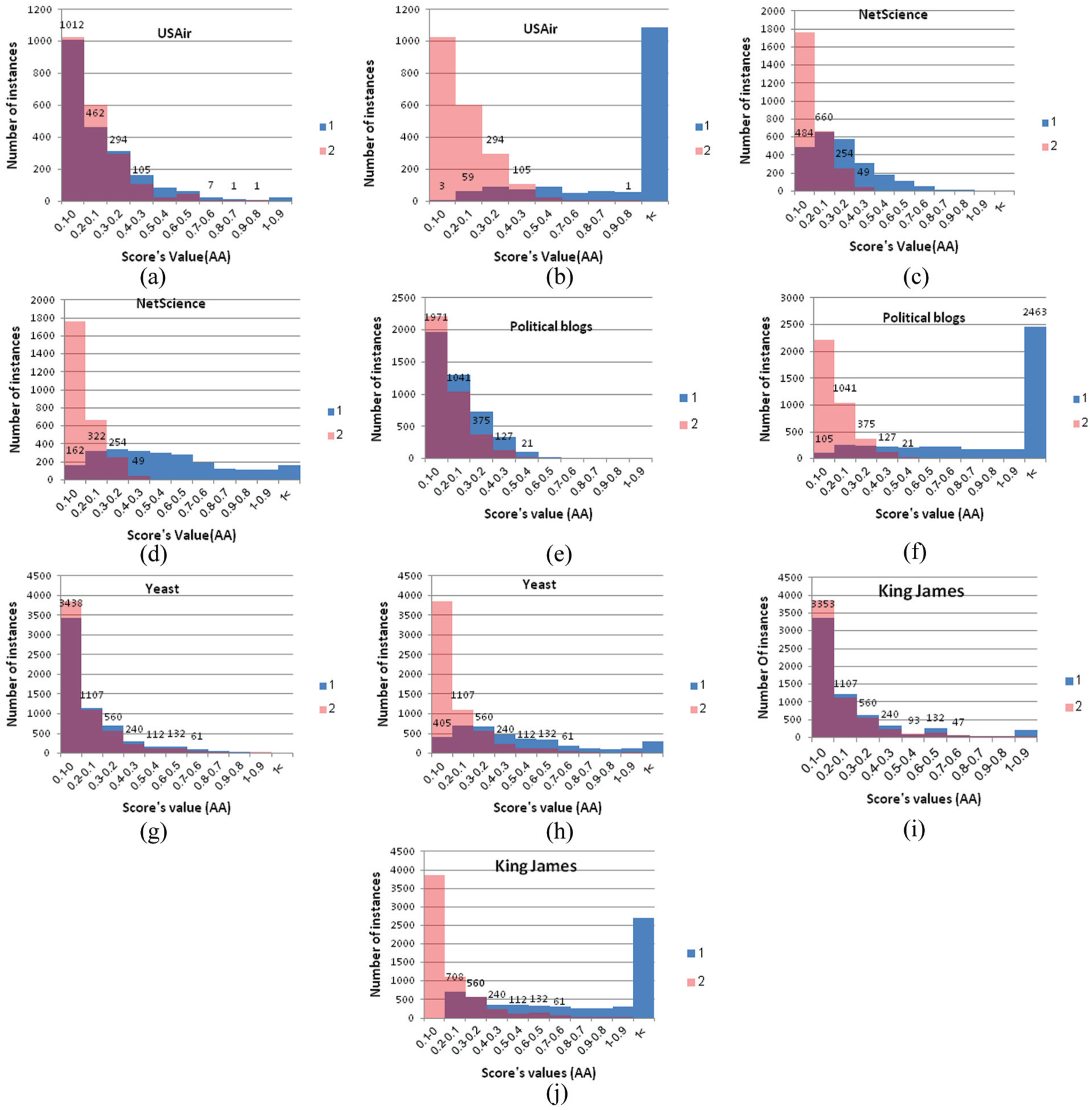
(a) The distribution of USAir dataset before weighting scores, (b) the distribution of USAir dataset after feature’s weighting, (c) the distribution of NetScience dataset before feature’s weighting, (d) the distribution of NetScience dataset after feature’s weighting, (e) the distribution of Political blogs dataset before feature’s weighting, (f) the distribution of Political blogs dataset after feature’s weighting, (g) the distribution of Yeast dataset before feature’s weighting, (h) the distribution of Yeast dataset after feature’s weighting, (i) the distribution of King James dataset before feature’s weighting and (j) the distribution of King James dataset after feature’s weighting.
5.4. Under-sampling data instances
As described in Section 3.1.3., to solve the imbalance in the dataset, some instances of the major class (non-existed edges) should be discarded. As a result, a balance is achieved.
5.5. Feature selection
In order to increase the quality of the evaluation results, feature selection is required. This is done by using GA as a feature’s filter as described in Section 3.1.4.
Table 5 shows summery of each benchmark dataset. This summery includes number of nodes and edges of the original dataset, number of instances resulted from under-sampling process, and suitable subset of features, for each dataset, resulted from feature selection process. After applying feature selection, USAir, NetScience, Political Blogs, Yeast and King James datasets will have four, three, four, five and four number of features, respectively. Narrowing down features number for each dataset depending on feature selection helps improving the prediction results latterly in the prediction stage. Each selected feature is checked with a tick under it with respect to the dataset. AA is for Adamic/Adar, CN for Common Neighbour, RA for Resource Allocation, PA for Preferential Attachment, JC for Jaccard Coefficient, GD for Graph Distance and PF for PropFlow. As a result, five processed datasets are ready for EVO-LP algorithm.
The original datasets details (number of nodes and edges) and their resulted number of instances and selected features.

AA: Adamic/Adar; CN: Common Neighbour; RA: Resource Allocation; PA: Preferential Attachment; JC: Jaccard Coefficient; GD: Graph Distance; PF: PropFlow.
Each selected feature is checked with a tick.
6. Experimental results and discussions
In this section, the results of implementing EVO-LP using the five processed datasets are presented, evaluated and discussed. All experiments are implemented in MATLAB R2017a and conducted using Intel® Core™ i7-5500 CPU @ 2.40 GHz processor, 8.00GB RAM, and Microsoft Windows8 of 64-bit Operating System.
The evolutionary algorithms: MFO, MFO2, MFO3, WOA, GA, PSO and DE, are chosen, as an optimised for EVO-LP, to test their prediction quality and conduct a comparison between them. Hence there are MFO-LP, MFO2-LP, MFO3-LP, GA-LP, PSO-LP, WOA-LP and DE-LP algorithms for testing. In addition, AA, which is one of the traditional similarity–based link prediction methods, is implemented and compared with EVO-LP results. AA is chosen for comparison, because it is one of traditional link prediction methods that performs surprisingly well [2].
For each EVO-LP algorithm, the population size is set to 50, the maximum number of iterations is set to 200 and the stopping criteria are the maximum number of iterations. Each EVO-LP algorithm had been executed 30 times independently. We focus on testing the prediction quality measured by the misclassification rate (cost function) and computing the performance metrics such as recall, G-mean, AUC, entropy and the computational time. Each of these measurements is stored for each independent 30 runs, and the best, average and standard deviation values are taken among these runs.
6.1. Cost function
As described in Section 3.2.3., misclassification rate is the cost function used to evaluate algorithm’s solution obtained so far. Lowest misclassification rate for one algorithm means highest prediction quality among other algorithms. Table 6 shows the misclassification rate for each EVO-LP algorithm applied on the five processed datasets. The Best, Average and STDEV represent the best, average and standard deviation of misclassification rate over 30 independent runs, respectively. In Table 6, the lowest Best, Average and STDEV are emphasised in bold-face. Bold STDEV represents the best standard deviation over EVO-LP algorithms, while the underlined represent the best standard deviation among all the algorithms including AA.
The misclassification rate for each EVO-LP algorithm.
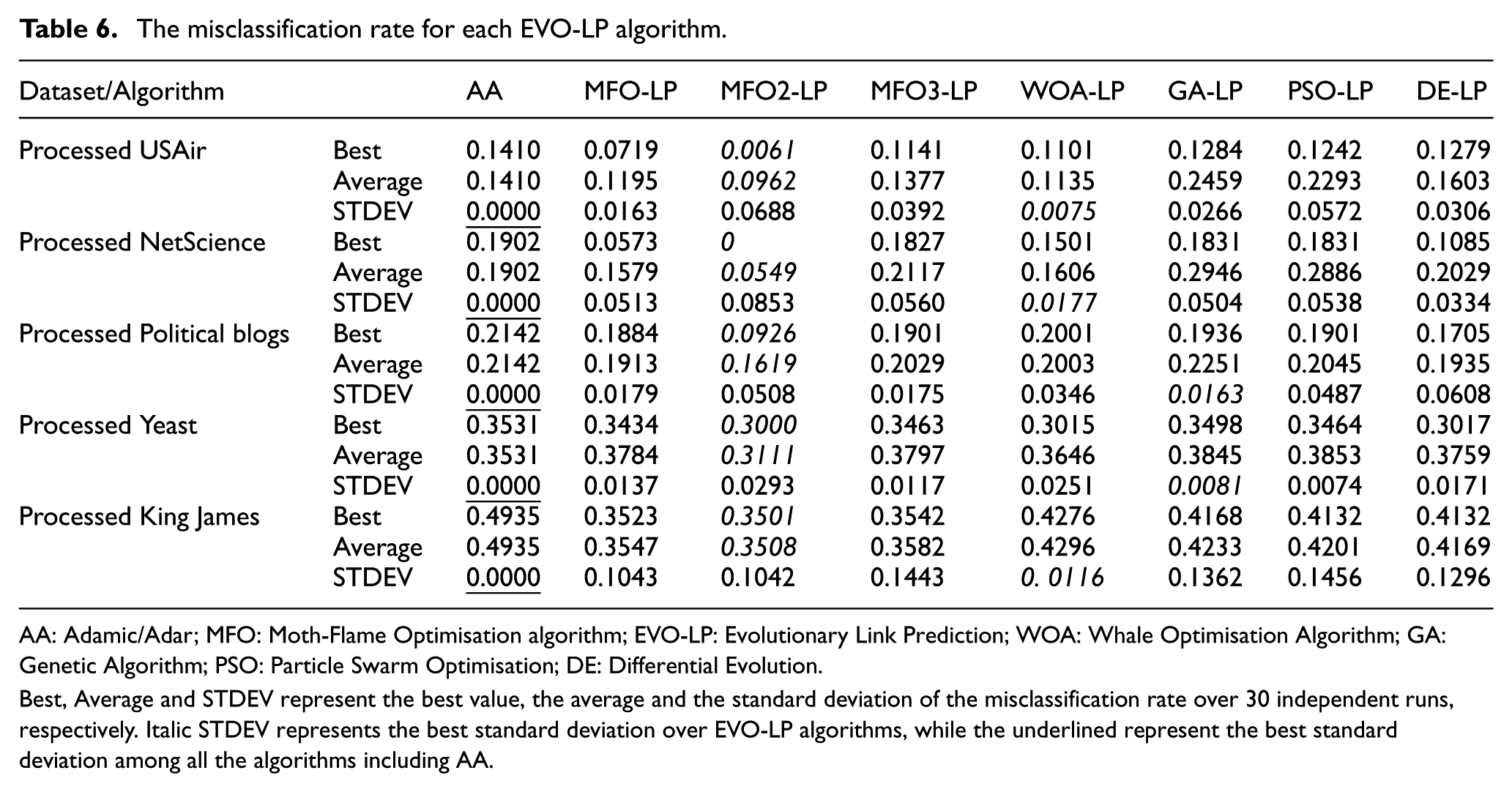
AA: Adamic/Adar; MFO: Moth-Flame Optimisation algorithm; EVO-LP: Evolutionary Link Prediction; WOA: Whale Optimisation Algorithm; GA: Genetic Algorithm; PSO: Particle Swarm Optimisation; DE: Differential Evolution.
Best, Average and STDEV represent the best value, the average and the standard deviation of the misclassification rate over 30 independent runs, respectively. Italic STDEV represents the best standard deviation over EVO-LP algorithms, while the underlined represent the best standard deviation among all the algorithms including AA.
As shown in Table 6, all EVO-LP algorithms (MFO-LP, MFO2-LP, MFO3-LP, WOA-LP, GA-LP, PSO-LP, DE-LP) have average misclassification rate scores lower than that for traditional method AA. Among all EVO-LP algorithms, MFO2-LP has the lowest average misclassification rate score. Even for the largest King James dataset, the MFO2-LP is still the best with 0.3508, while the other algorithms get average misclassification rate scores from 0.3547 to 0.4296. MFO2-LP has a standard deviation not as good as that for other algorithms. This means MFO2-LP is less stable than other EVO-LP algorithms. AA has a 0 standard deviation because it is not a meta-heuristic algorithm and gives same results for each independent run for the same set of data.
From Tables 5 and 6, we can find that the misclassification rate scores of the datasets are proportional to their number of instances; an algorithm can get better misclassification rate on datasets with lesser number of instances.
Figure 13(a)–(d) indicates the behaviour of each EVO-LP algorithms during their iterations until getting the best solution that has the lowest misclassification rate. If we take a look at these figures, MFO2-LP clearly has the fastest convergence behaviour among other algorithms across the majority of the datasets. So, it has the ability to find the best solution early in comparison with other EVO-LP algorithms because it uses the hyperbolic (reciprocal) spiral to update search space instead of the logarithmic spiral found in the original MFO. DE-LP is the slowest. MFO-LP, MFO3-LP, GA-LP, PSO-LP and WOA-LP have a convergence speed and behaviour approximately close to each other.

(a) The convergence curves of misclassification rate for each EVO-LP algorithms applied on the processed USAir dataset, (b) the convergence curves of misclassification rate for each EVO-LP algorithms applied on the processed NetScience dataset, (c) the convergence curves of misclassification rate for each EVO-LP algorithms applied on the processed Political blogs dataset and (d) the convergence curves of misclassification rate for each EVO-LP algorithms applied on the processed Yeast dataset.
6.2. Performance metrics
To evaluate the quality of the prediction results, performance metrics such as recall, G-mean, AUC, entropy and computational time are computed for each EVO-LP algorithm over the five processed datasets and 30 independent runs.
6.2.1. Recall
Recall measures how precise and how complete the classification is on the positive class, the existed edges. We need to measure recall which helps to quantify how much is the TPR in the prediction results. If we have high recall, then we can guarantee high values for AUC and G-mean. Highest recall for one algorithm means highest prediction quality among other algorithms. Table 7 shows the recall for each EVO-LP algorithm applied on the five processed datasets. The Best, Average and STDEV represent the best, average and standard deviation of recall over 30 independent runs, respectively. In Table 7, the highest Best and Average are emphasised in bold-face. Bold STDEV represent the best standard deviation over EVO-LP algorithms, while the underline STDEV represents the best standard deviation among all algorithms including AA.
The recall for each EVO-LP algorithm.
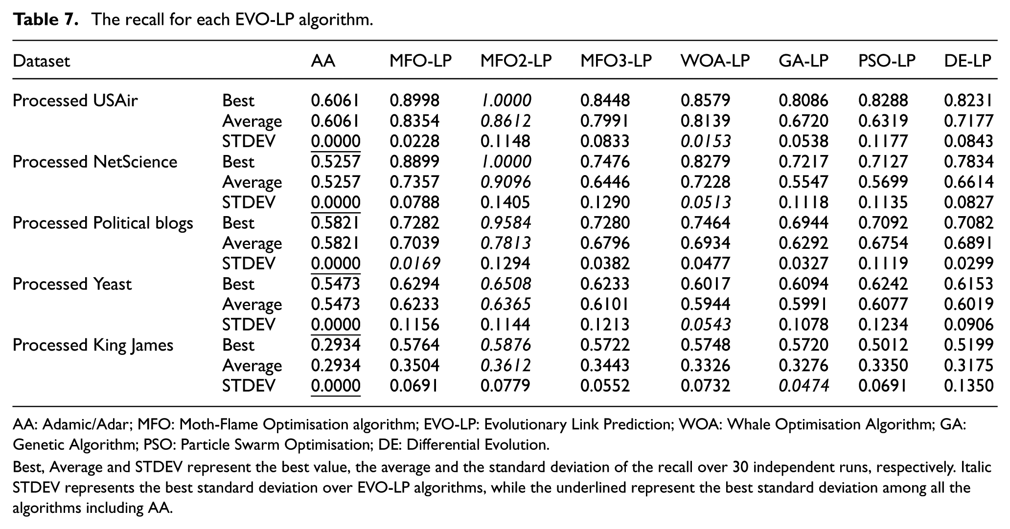
AA: Adamic/Adar; MFO: Moth-Flame Optimisation algorithm; EVO-LP: Evolutionary Link Prediction; WOA: Whale Optimisation Algorithm; GA: Genetic Algorithm; PSO: Particle Swarm Optimisation; DE: Differential Evolution.
Best, Average and STDEV represent the best value, the average and the standard deviation of the recall over 30 independent runs, respectively. Italic STDEV represents the best standard deviation over EVO-LP algorithms, while the underlined represent the best standard deviation among all the algorithms including AA.
As shown in Table 7, all EVO-LP algorithms have average recall scores higher than that for the traditional method AA. Among all EVO-LP algorithms, MFO2-LP has the highest average recall score. Even for the largest King James dataset, the MFO2-LP is still the best with 0.3612, while the other algorithms get average recall scores from 0.3175 to 0.3504, but MFO2-LP has a standard deviation not as good as that for other algorithms.
6.2.2. G-mean
The G-mean measures the balanced performance of a learning algorithm between positive class (class1: existed edges) and negative class (class2: non-existed edges). Highest G-mean for one algorithm means highest prediction quality among other algorithms. Table 8 shows the G-mean for each EVO-LP algorithm applied on the five processed datasets.
The G-mean for each EVO-LP algorithm.
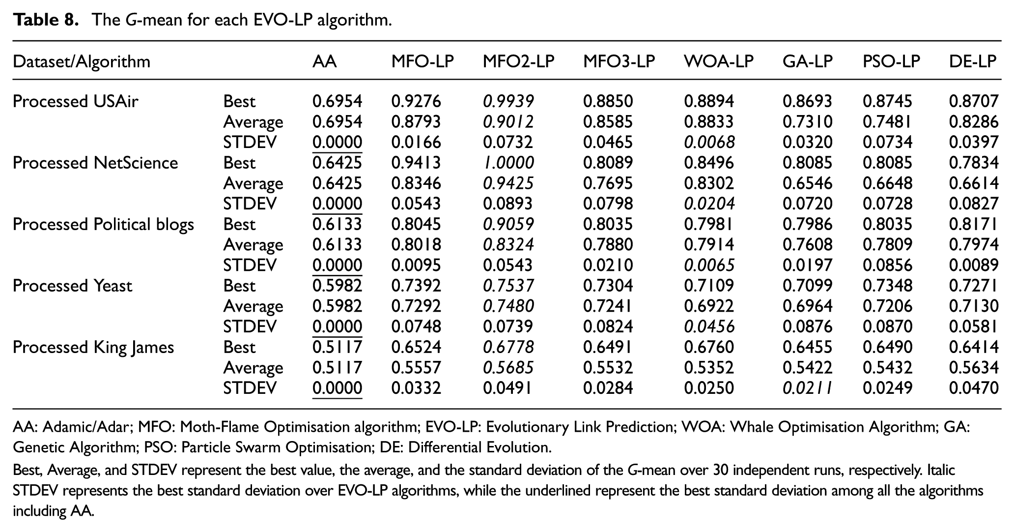
AA: Adamic/Adar; MFO: Moth-Flame Optimisation algorithm; EVO-LP: Evolutionary Link Prediction; WOA: Whale Optimisation Algorithm; GA: Genetic Algorithm; PSO: Particle Swarm Optimisation; DE: Differential Evolution.
Best, Average, and STDEV represent the best value, the average, and the standard deviation of the G-mean over 30 independent runs, respectively. Italic STDEV represents the best standard deviation over EVO-LP algorithms, while the underlined represent the best standard deviation among all the algorithms including AA.
As shown in Table 8, all EVO-LP algorithms have average G-mean scores higher than that for the traditional method AA. Among all EVO-LP algorithms, MFO2-LP has the highest average G-mean score, because MFO2-LPs has the highest recall. Even for the largest King James dataset, the MFO2-LP is still the best with 0.5685, while the other algorithms get average G-mean scores from 0.5352 to 0.5634. On the contrary, WOA-LP has the best standard deviation over other algorithms.
6.2.3. AUC
Greater AUC means better prediction model. Highest AUC for one algorithm means highest prediction quality among other algorithms. Table 9 shows the AUC for each EVO-LP algorithm applied on the five processed datasets.
The AUC for each EVO-LP algorithm.
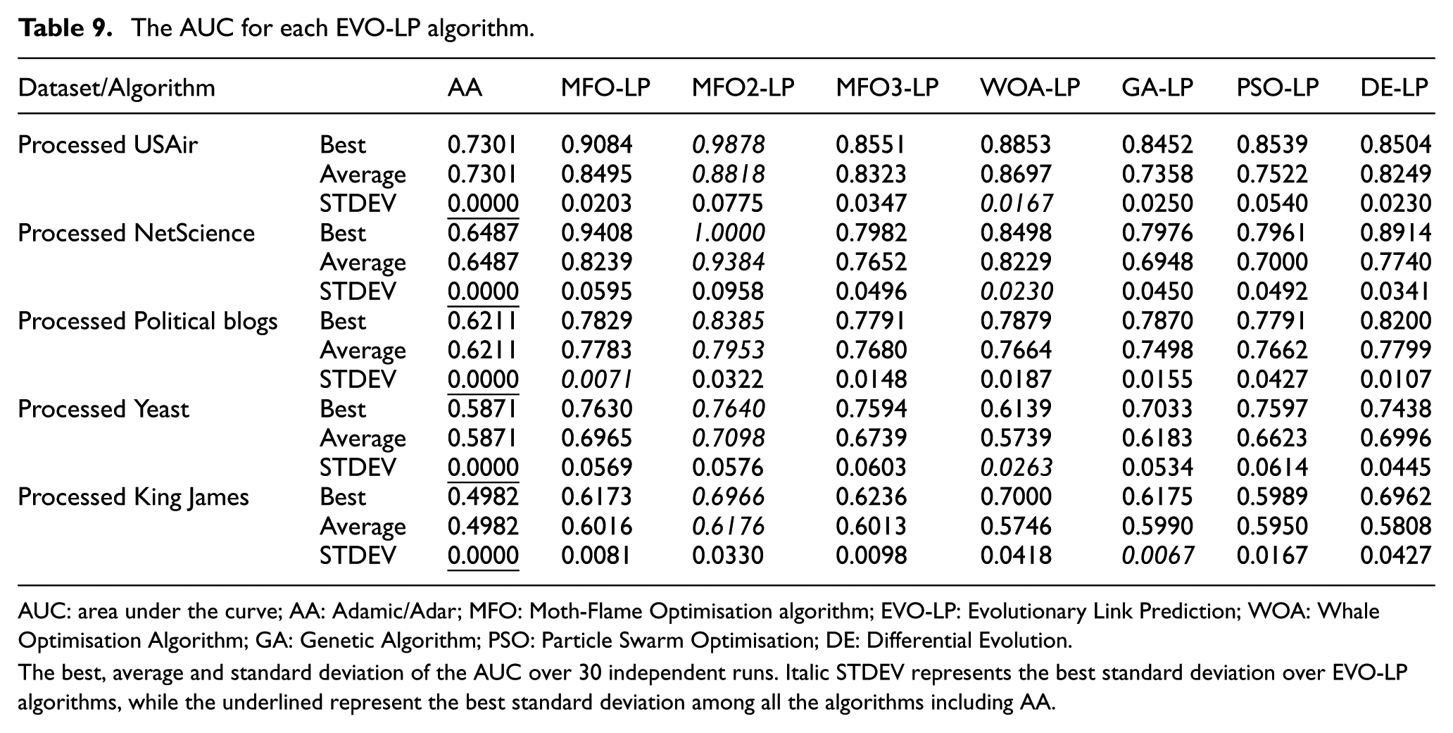
AUC: area under the curve; AA: Adamic/Adar; MFO: Moth-Flame Optimisation algorithm; EVO-LP: Evolutionary Link Prediction; WOA: Whale Optimisation Algorithm; GA: Genetic Algorithm; PSO: Particle Swarm Optimisation; DE: Differential Evolution.
The best, average and standard deviation of the AUC over 30 independent runs. Italic STDEV represents the best standard deviation over EVO-LP algorithms, while the underlined represent the best standard deviation among all the algorithms including AA.
As shown in Table 9, all EVO-LP algorithms have average AUC scores higher than that for the traditional method AA. Among all EVO-LP algorithms, MFO2-LP has the highest average AUC score. This is due to the large value of MFO2-LP’s recall, which means large TPR, and then large AUC. Even for the largest King James dataset, the MFO2-LP is still the best with 0.6176, while the other algorithms get average AUC scores from 0.5808 to 0.6016. The WOA-LP has the best standard deviation over other algorithms.
6.2.4. Entropy
Better prediction results can be obtained, when Entropy becomes closer to zero. Lowest entropy for one algorithm means highest prediction quality among other algorithms. Table 10 shows the entropy for each EVO-LP algorithm applied on the five processed datasets. As shown in Table 10, all EVO-LP algorithms have average entropy scores lower than that for the traditional method AA. Among all EVO-LP algorithms, MFO2-LP has the lowest average entropy score. Even for the largest King James dataset, the MFO2-LP is still the best with 0.8089, while the other algorithms get average entropy scores from 0.8366 to 0.9406. The WOA-LP has the best standard deviation over other algorithms.
Entropy for each EVO-LP algorithm.
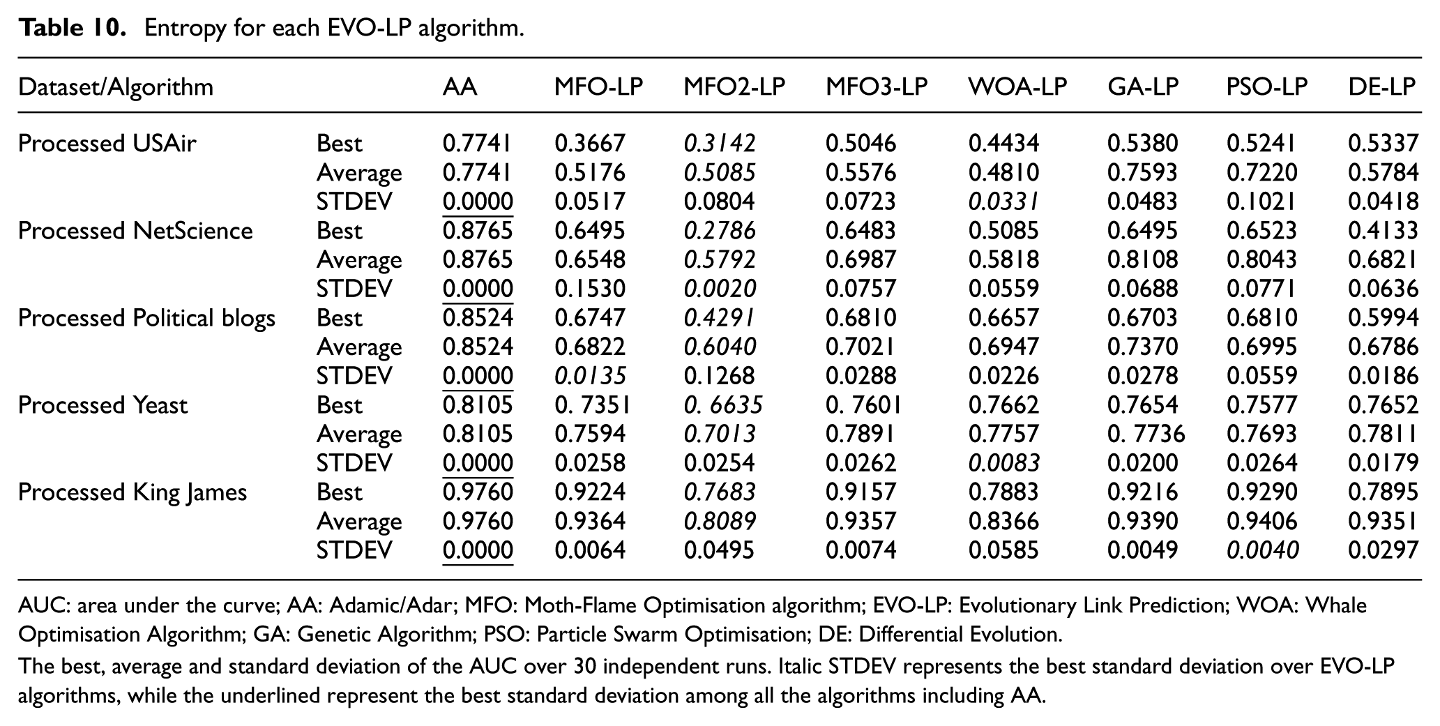
AUC: area under the curve; AA: Adamic/Adar; MFO: Moth-Flame Optimisation algorithm; EVO-LP: Evolutionary Link Prediction; WOA: Whale Optimisation Algorithm; GA: Genetic Algorithm; PSO: Particle Swarm Optimisation; DE: Differential Evolution.
The best, average and standard deviation of the AUC over 30 independent runs. Italic STDEV represents the best standard deviation over EVO-LP algorithms, while the underlined represent the best standard deviation among all the algorithms including AA.
6.2.5. Execution time
Figure 14 indicates the execution time for each algorithm over the five processed datasets. As shown from the figure, EVO-LP algorithms spend less time for execution in comparison with time spending by the traditional algorithm AA. As in formula (26), EVO-LP algorithms depend mainly on the number of instances in the processed datasets, while AA depends mainly on the number of nodes in the observed network. AA complexity is O(K2 N) [3], where K is the average degree and N is number of nodes in the network. Number of nodes in the network is usually much larger than the number of instances produced from preprocessing the network, as in our work. Therefore, EVO-LP algorithms performed faster than AA algorithm.
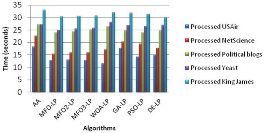
Execution time of the algorithms.
Over the EVO-LP algorithms, we can observe that MFO-LP and their versions MFO2-LP and MFO3-LP have the minimal execution time. This is because MFO-LP has a complexity of O(t s x), where t is the maximum iterations, s is the population size and x is the number of instances. Due to s and t are the same for each algorithm, x will affect the execution time. Comparing Table 5 with Figure 14, when the number of instances in the dataset increases, the execution time will increase proportionally.
7. Conclusion and future work
This study presents a meta-heuristic framework based on clustering and using a processed datasets for solving link prediction problem. This framework is divided into preprocessing stage and link prediction stage. For each stage, there are a number of experiments conducted, as discussed previously, and conclusions are built upon these experiments.
The merits of this study lie in each step of the methodology of EVO-LP framework. Each step can be considered valuable in itself and complement to other steps. This section discusses these merits as follows. To ensure the gradation in the number of instances in the processed dataset, a variety of networks from different fields, such as social, biological, information and publication networks, are selected with varied number of nodes and already existed edges. In our approach, the number of instances in the processed dataset depends on the already existed edges in the original network proportionally.
Furthermore, dividing the original dataset into training and testing sets supports the prediction process and takes the benefits of supervised learning besides the unsupervised learning that can be found in the prediction stage by using data clustering process. Choosing 80/20 ratio based on the Pareto Principle [52] was successful. EVO-LP algorithms proved their success in the prediction quality results and execution time.
In addition, dataset distribution helps in specifying whether instances of each class are disjoints or overlapped. Availability of overlapping in the dataset reduces the prediction quality. So, overlapping should be reduced as possible. Therefore, the weighting score process should be applied to increase both the recall and the specificity of the processed dataset’s classes. As a result, the overall prediction quality will be improved well.
Data under-sampling and feature selection are very important processes because both of them help in increasing the prediction quality. Under-sampling the major class leads to improve both recall, TPR of the first class (existed edge) and specificity, true negative rate for the second class (non-existed edges) and then prevents one class dominate other class. Therefore, the performance of prediction measured by G-mean and AUC will increase significantly.
Preprocessing stage makes the complexity of our approach depends on the number of instances in the processed dataset, not on the number of nodes or edges in the original dataset. This is the reason that EVO-LP algorithms outperform the traditional similarity–based link prediction methods such as AA in both prediction quality and execution time.
The misclassification rate was chosen as a cost function to evaluate the prediction result. As illustrated in Section 3.2.3, this result is produced by applying data clustering through using SSE. We let misclassification rate decides whether the prediction result is approved or not because we cannot just depend on SSE as a cost function. This is because in some cases we can have small SSE but with large misclassification rate.
Also, we focused to measure the recall which helps to quantify how much is the TPR in the prediction results. If we have high recall, then we can guarantee high values for AUC and G-mean. Highest recall for one algorithm means highest prediction quality among other algorithms.
The experimental results show that the misclassification rate scores of the datasets are proportional to their number of instances; an algorithm can get better misclassification rate on datasets with lesser number of instances. This brings our attention to the need for dividing the dataset instances into number of subsets and sends each subset to one processor in parallel approach.
EVO-LP was applied using number of well-regarded meta-heuristic algorithms which are MFO-LP, MFO2-LP, MFO3-LP, GA-LP, PSO-LP, WOA-LP and DE-LP. A comparison between these algorithms was conducted in terms of recall, G-mean, AUC, classification error rate, entropy and the execution time. The experimental results show that applying MFO2-LP for link prediction outperforms other regarded meta-heuristic algorithms in terms of prediction results and execution time. Consequently, utilising the MFO2 for EVO-LP framework to produce MFO2-LP achieves the best prediction results in a reasonable amount of time.
Finally, processing dataset as in this work, make the dataset composed of number of rows. Each row represents an instance. These instances are independent of each other. This composition of processed dataset facilitates the division process into number of subsets. So, each subset can contain number of rows easily. By division, we can get higher prediction quality and less execution time. This division can be done through applying parallel approach and distribute each subset of data on processors. It is our future work to develop parallel EVO-LP for link prediction problem efficient in both prediction quality and execution time.
Footnotes
Declaration of conflicting interests
The author(s) declared no potential conflicts of interest with respect to the research, authorship and/or publication of this article.
Funding
The author(s) received no financial support for the research, authorship and/or publication of this article.