A semantic-based video scene segmentation using a deep neural network

Abstract

Video scene segmentation is very important research in the field of computer vision, because it helps in efficient storage, indexing and retrieval of videos. Achieving this kind of scene segmentation cannot be done by just calculating the similarity of low-level features presented in the video; high-level features should also be considered to achieve a better performance. Even though much research has been conducted on video scene segmentation, most of these studies failed to semantically segment a video into scenes. Thus, in this study, we propose a Deep-learning Semantic-based Scene-segmentation model (called DeepSSS) that considers image captioning to segment a video into scenes semantically. First, the DeepSSS performs shot boundary detection by comparing colour histograms and then employs maximum-entropy-applied keyframe extraction. Second, for semantic analysis, using image captioning that benefits from deep learning generates a semantic text description of the keyframes. Finally, by comparing and analysing the generated texts, it assembles the keyframes into a scene grouped under a semantic narrative. That said, DeepSSS considers both low- and high-level features of videos to achieve a more meaningful scene segmentation. By applying DeepSSS to data sets from MS COCO for caption generation and evaluating its semantic scene-segmentation task results with the data sets from TRECVid 2016, we demonstrate quantitatively that DeepSSS outperforms other existing scene-segmentation methods using shot boundary detection and keyframes. What’s more, the experiments were done by comparing scenes segmented by humans and scene segmented by the DeepSSS. The results verified that the DeepSSS’ segmentation resembled that of humans. This is a new kind of result that was enabled by semantic analysis, which was impossible by just using low-level features of videos.

Keywords

Deep learning image captioning keyframe extraction shot boundary detection video scene segmentation

1. Introduction

Video is one of the most commonly used multimedia data along with image and audio. With the rise of information technology, video data’s volume has increased exponentially [1,2]. Because of the high acceleration of the networks, providing real-time streaming for high-quality video became possible, which led to an increase in the users who enjoy video content and to the significant growth of companies that deal with video content, such as YouTube and Facebook, as various video contents were consumed by the increased user base [3,4]. With this increase in the demand for video data, constant efforts have been made to understand and analyse them to produce high-quality video contents as well as to develop search engines and recommendation systems for high-quality video content [2 –5].

When dealing with such large amounts of visual data, efficient and effective management is an important challenge [6 –9]. To do this, effective methods of processing, organising, summarising and indexing in a semantically meaningful manner are required. When processing videos, a video shot is usually taken as the basic unit. Currently, shot detections on various transitions are now quite reliable [10,11]. Nonetheless, to process video tasks on higher levels, obtaining a description of scenes for videos is a crucial need. The definition of a video scene is as follows: a unit that constitutes a group of continuous shots sharing a flowing narrative and concept. The very nature of the scene itself is based much more on semantic structures than are shots. Video scene segmentation is the process of partitioning a video into a set of shots grouped under a common semantic meaning; it has countless applications, such as video summarisation and retrieval [6,12].

Although many studies have reported satisfactory performance in video scene segmentation, they mostly struggle to provide the users with the scene they desired from the video, because they overlook the semantic elements of shots and keyframes and focus more on detecting scenes by means of low-level features [2 –4]. Thus, in this article, we propose a Deep-learning Semantic-based Scene-segmentation model (called DeepSSS) that considers image captioning to segment a video into scenes semantically by detecting and generating semantic information from shots and keyframes in the video. In other words, high-level features, aside from low-level features, have been taken into consideration to generate a more meaningful scene segmentation. What makes DeepSSS unique is that, unlike existing scene-segmentation approaches, it attempts to detect the semantic information embedded in the shots and keyframes, extract it from the video and analyse it. To do so, DeepSSS benefits from a method that generates text to describe keyframes and uses it to compare similarities between keyframes, a cutting-edge technique that has been made possible by deep learning. As a result, DeepSSS advances beyond existing approaches by extracting semantic relationships between shots and using this data to segment videos into scenes semantically.

The structure of this article is as follows: section 2 presents contemporary trends and research about existing scene segmentation and detection. Section 3 provides a specific description of DeepSSS. Section 4 illustrates the performance and experimental results of our proposed model. Finally, section 5 provides discussion and conclusion.

2. Related research

During the last decade, many researchers have worked on scene segmentation. For example, Rasheed and Shah [13] proposed a method of using a two-pass algorithm to detect scenes within movies and TV shows, where the initial pass uses backward shot coherence, detecting scene boundaries based on colour histogram similarities between the shots presented in the window. The second pass, however, merges the segmented parts into larger scenes based on each scene’s similarity in motions to retain more continuity throughout each scene.

In a similar attempt by Rasheed and Shah [14], a shot similarity graph (SSG) was used. The SSG, a weighted undirected graph, then computes the similarities between nodes while using the similarities between nodes as weights in the graph based on each node’s colour histogram and motion information. The SSG, using a normalised-cut method, is then split into smaller story units [15]. This is a divisive method, unlike the previous one, to segment the movie into scenes.

A temporal video segmentation was proposed by Zhai and Shah [16]. This method initialised an arbitrary number of scene boundaries, which are automatically updated with diffusion and jumps. A Markov Chain Monte Carlo process controls the updates of the model parameters. Many of these methods depend on local or global constraints. Gu et al. [17] reported that local temporal continuity should be considered as much as the global distribution of time and content. In an energy-maximisation-based segmentation (EMS) proposed by Gu and colleagues, content and context energy represent the global and local constraints. The energies are then optimised in two steps. In order to estimate the initial scene label values, content energy is modelled using energy maximisation (EM) to fit a generative model, which is then followed with the iterative conditional modes (ICMs). The ICM is used to find global optimisation using context energy.

The selection of proper features, such as colour, texture, motion vectors and appropriate distance-measuring methods, were traditionally the most efficient methods that video segmentation has relied on [18,19]. Selecting different features or focusing on different homogeneities resulted in drastically different scene-segmentation results, even for the same videos. With segmentations usually obtained at shot level, previous scene segmentations mostly relied on similarities across shots, whereas previous approaches [13,14] used a colour histogram as the main computing feature and used a single-length path that considered only pairwise similarity to measure the continuity between shots.

In a recent attempt, Lu et al. [20] proposed a scene-detection method specifically for automatic summarisation of surveillance videos. The problem with the approach is that, if performed on data sets different from the one originally used, the accuracy of the results degrades greatly. However, our proposed model (which is a visual–text hybrid in nature), unlike previous existing methods, can work on various videos in different domains, since it uses a text-generation method (by benefitting from deep neural networks) that describes an image to extract semantic information from the extracted keyframes for scene detection.

3. DeepSSS: Deep-learning Semantic-based Scene-segmentation model

Figure 1 illustrates the overall architecture of our proposed model (called DeepSSS), including four distinct stages. The first stage is shot boundary detection (see section 3.1); it detects shots from the video and extracts them. Next is keyframe extraction (see section 3.2); it extracts keyframes that represent the shot from the shots we got in the previous stage. Third, a line of text describing the extracted keyframes is generated (see section 3.3). These texts are used to analyse the keyframes’ semantic elements and compare their similarities to each other. The final stage is scene assembly (see section 3.4); the generated texts along with the extracted keyframes are used to calculate the similarities between shots and then assemble them, completing the proposed model.

Figure 1.

Architecture of the DeepSSS.

3.1. Shot boundary detection

Shot boundary detection is the most common and fundamental task in video analysis. In this task, shot boundaries are extracted from the full video. Generally, a video is structured hierarchically and consists of frames, shots and scenes. Shots are structured by a continuous flow of frames, and frames within those shots have strong correlations with each other [21]. Therefore, a shot is the most basic unit that can have semantic information among the elements constituting video contents.

Normally, a shot boundary is detected according to the transitions between shots, which can be divided into sudden transitions, which happen between shots, such as cut transition, dissolve, fade in/out and wipe, and gradual transition, which performs the transitions gradually [22]. The method of shot boundary detection is as follows: (1) extract features from each frame, (2) calculate the similarities between each frame from the extracted features and (3) detect the shot boundary by detecting the frame that sticks out from the other frames in the flow.

For shot boundary detection in DeepSSS, we used an RGB (Red, Green, Blue) colour histogram, which provides the distribution of RGB colours from the pixels of the whole frame. The histogram of each colour channel has been generated using the following equations

His t_{C} (I) = \sum_{a = 1}^{m} \sum_{b = 1}^{n} F (a, b)

(1)

where C = R, G or B; I is the extracted frame; the size of the frame is m × n; and F(a, b) is the intensity of the colour channel C at position (a, b). The similarities between frames are calculated by means of the distances between the calculated histograms. In this article, we have also used the separation between classes as a means of measurement for the pattern classification task and used the Bhattacharyya distance (equation (2)), which provides useful information when extracting features, when calculating the similarities between frames [23]

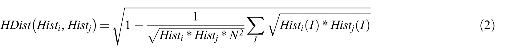
HDist (His t_{i}, His t_{j}) = \sqrt{1 - \frac{1}{\sqrt{His t_{i} * His t_{j} * N^{2}}} \sum_{I} \sqrt{His t_{i} (I) * His t_{j} (I)}}

(2)

Here, the distance value shall be 0 if the two frames are alike and 1 if the two frames are completely different

\sum_{i = 1}^{n} HDist (His t_{i}, His t_{i + 1}) = {\begin{matrix} 1 & if Dist > γ \\ 0 & else \end{matrix}

(3)

In shot boundary detection, if the result of equation (2) is greater than or equal to the fixed threshold value γ, we consider that the two frames differ in colour distribution and consider it a shot boundary (equation (3)). In this article, we set the γ value as 0.25, since we could confirm that the best performance was obtained with it.

3.2. Keyframe extraction

In this section, we extract the keyframes that represent the shots extracted through shot boundary detection. Since colour is not greatly affected by the spins or movement of the input image, it is one of the most key features in image processing. To represent colour, we use colour spaces, such as RGB and HSI (Hue, Saturation, Intensity). Colour-histogram-based techniques such as these are faster than shape or texture techniques.

For keyframe extraction, we calculate the entropy of each frame in the shot and select the maximum-entropy frame within each shot as a keyframe (equation (4))

Ent (I) = - \sum_{i} (p_{i} lo g_{2} (p_{i}))

(4)

Value p is the histogram for intensity frame I.

3.3. Extracting semantic information form keyframe

Recently, there have been various propositions for using deep learning to analyse images [24], and various studies (such as Vinyals et al. [25] and Wang et al. [26]) on image-captioning techniques, generating texts that describes the image, have been in progress. In this case, the generated text gives a semantic description about the image. Therefore, we have established the following hypothesis:

Hypothesis. A semantically similar frame will generate a semantically similar text description.

Then, we can generate text descriptions from the keyframe to analyse the semantic similarities between keyframes that represent each shot, therefore comparing the semantic similarities between shots. In this article, a deep-learning-based method of generating text describing the content from an image has been applied to the DeepSSS to semantically analyse keyframes and thereby detect semantic scenes.

For text generation, DeepSSS has applied the text-generating method using long short-term memory (LSTM) proposed by Wang et al. [26]. An LSTM is a variation of a recurrent neural network (RNN), which performs well in machine translation [27], speech recognition [28], sequence generation [29] and so on. An LSTM model is composed of cells with multiple gates attached, and the cells behave in several ways, depending on the values of the gates that each cell is connected to. In short, the weights are trained on the same principle of how a value of a hidden layer is trained, and the learning process uses a gradient descent that uses the output error. The LSTM is a memory cell C that encodes the knowledge at all stages of the observed input up to the current stage (Figure 2).

Figure 2.

LSTM memory block.

The cell is controlled by the gate. In this layer, multiplication is applied; therefore, if the gate value is 1, then the gated layer’s value is kept, but if the gate value is 0, then the gated layer’s value becomes 0. Three gates are being used to control whether to forget the current cell value (forget gate f), if it should read its input (input gate i), or whether to output the new cell value (output gate o). The definition of gate, cell update and output is as follows (equations (5)–(10))

i_{t} = σ (W_{ix} x_{t} + W_{im} m_{t - 1})

(5)

f_{t} = σ (W_{fx} x_{t} + W_{fm} m_{t - 1})

(6)

o_{t} = σ (W_{ox} x_{t} + W_{om} m_{t - 1})

(7)

c_{t} = f_{t} ⊙ c_{t} + i_{t} ⊙ h (W_{cx} x_{t} + W_{cm} m_{t - 1})

(8)

m_{t} = o_{t} ⊙ c_{t}

(9)

p_{t + 1} = softmax (m_{t})

(10)

The ⊙ represents the product with a gate value, and the various W matrices are the trained parameters. The nonlinearities are sigmoid (·) and hyperbolic tangent h (·). The final equation, m_t, is used to feed a Softmax, producing a probability distribution p_t over all words.

The LSTM is trained to predict each word after the sentence after it has seen the image as well as all preceding words as defined by p(S_t|I, S₀, …, S_{(t − 1)}). For all LSTMs to share the same parameters and for the output m_{(t − 1)} of LSTM at the time of t − 1 to be fed to the LSTM at the time of t, a copy of the LSTM memory is created for the image and sentence word (Figure 3).

Figure 3.

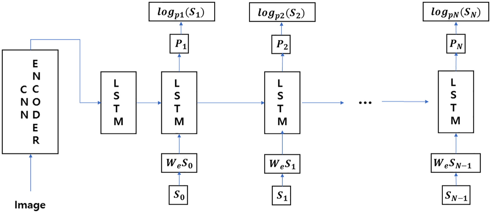
LSTM model for sentence generation.

All recurrent connections are transformed into unrolled versions of feed-forward connections. In other words, if we denote the input image and S = (S₀, …, S_N) as a text description of the image, the unrolling procedures is read as follows (equations (11)–(13))

x_{- 1} = CNN (I)

(11)

x_{t} = W_{e} S_{t}, t \in {0, \dots, N - 1}

(12)

p_{t + 1} = LSTM (x_{t}), t \in {0, \dots, N - 1}

(13)

Here, we represent each word as a one-shot vector S_t, with the vector’s dimension equal to the size of the dictionary. A special start word and special end word are denoted as S₀ and S_N, respectively, to designate the boundaries of each text string. The end word S_N also functions to facilitate the LSTM signal that a complete text is generated as a full sentence. Both the image and the word are mapped on the same space. This happens as the image is done using vision convolutional neural network (CNN) and the words are done using word embedding. The image I is input only once at time t =−1. In Vinyals et al. [25], it was verified that feeding the image at each time step as an extra input yields inferior results, because the network can explicitly exploit noises in the image and overfits more easily. The loss is the sum of negative log likelihood of correct words for each stage (equation (14))

L (I, S) = - \sum_{t = 1}^{N} lo g_{pt} (S_{t})

(14)

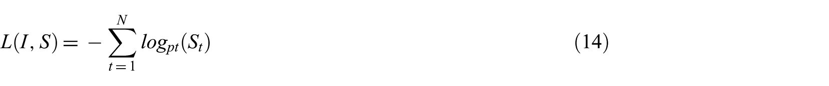
The loss above can be minimised for all of the LSTM’s parameters, image embedding CNN and word embeddings, W_e. The image–text pair set’s training proceeds through the model above. Once the training is finished, the DeepSSS generates a text description of the image. The text represents the image semantically through a new text description with the word-by-word format.

3.4. Assemble scene

In this section, we finally calculate the similarities between keyframes and assemble the shots to scenes, completing our scene-segmentation process. To do this final process, we should solve the following problems. The first is when the shots are semantically connected to the same scene yet have drastically different histograms from the surrounding shots. These kinds of problems usually occur when the scene in the video is colourful and dynamic. The second is the opposite of the first one; when the shots are not semantically linked yet the histogram is similar. This usually happens in video contents such as documentaries. The solution for these kinds of problems was to calculate the similarities from the histogram and the generated texts. Although the problems above cannot be solved using histograms alone, it can be solved using the generated texts, since the semantic information is embedded in those texts.

Similarity comparison for the generated text describing keyframes can be done by extracting its parts of speech through part-of-speech tagging. From the extracted parts of speech, we have used the nouns only (NN), adjectives (JJ) and verbs (VB) for calculating similarities. For calculating similarities between the extracted texts, we applied the Jaccard similarity method (equation (15))

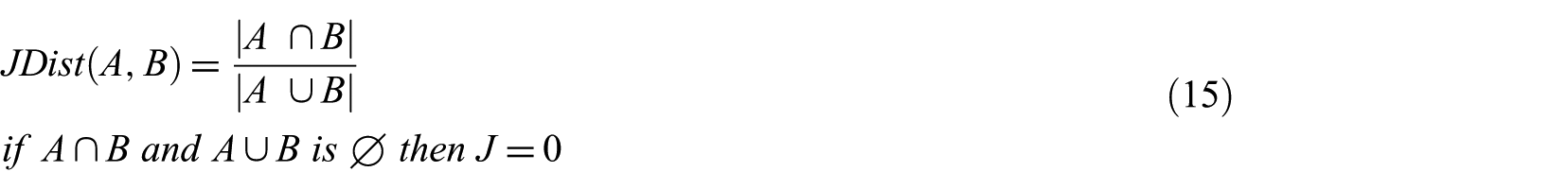
\begin{matrix} JDist (A, B) = \frac{| A \cap B |}{| A \cup B |} \\ if A \cap B and A \cup B is \emptyset then J = 0 \end{matrix}

(15)

A and B are the result sets of the generated texts from each frame passed through the part-of-speech tagging process. The value becomes closer to 1 as the texts become more similar, but if the texts become more different, the value converges to 0. Originally, in Jaccard similarity, when both the denominator and the numerator are empty, the value is 1. In contrast, in this article, because when the generated texts are similar, the value converges to 1, and when the denominator and numerator are empty, the similarity between texts cannot be calculated; we have proposed that if the denominator and numerator are both empty, the value will be 0 to prevent any contradictions.

To assemble the shots into scenes, the similarity of the two keyframes is calculated through both histogram and text. If the calculated difference is higher than the threshold value, the scene is divided. Table 1 shows the framework for scene assembly.

Table 1.

Scene assembly algorithm.

Input: Pair of keyframes, Pair of generated textsOutput: Scenes
1 Read all keyframe and sentence pairs 2 Start_point, end_point 3 For i = 1: n 4 Calculate RGB histogram of frame i and i + 1 5 Calculate $HDist (Keyfram e_{i}, Keyfram e_{i + 1})$ 6 Calculate $JDist (Sentenc e_{i}, Sentenc e_{i + 1})$ 7 if ( $ADist (HDist, JDist) ⩽ θ$ ) 8 put $Fram e_{i}$ in end_point 9 i = j 10 break 11 else if( $ADist (HDist, JDist) ⩽ θ$ )and i < mini_count 12 continue 13 else 14 put $Fram e_{i + 1}$ in end_point 15 put i to i + 1 in scene 16 put $Fram e_{i + 1}$ in start_point 17 end

Input: Pair of keyframes, Pair of generated textsOutput: Scenes

1 Read all keyframe and sentence pairs
2 Start_point, end_point
3 For i = 1: n
4 Calculate RGB histogram of frame i and i + 1
5 Calculate

HDist (Keyfram e_{i}, Keyfram e_{i + 1})

6 Calculate

JDist (Sentenc e_{i}, Sentenc e_{i + 1})

7 if (

ADist (HDist, JDist) ⩽ θ

)
8 put

Fram e_{i}

in end_point
9 i = j
10 break
11 else if(

ADist (HDist, JDist) ⩽ θ

)and i < mini_count

12 continue
13 else
14 put

Fram e_{i + 1}

in end_point
15 put i to i + 1 in scene
16 put

Fram e_{i + 1}

in start_point
17 end

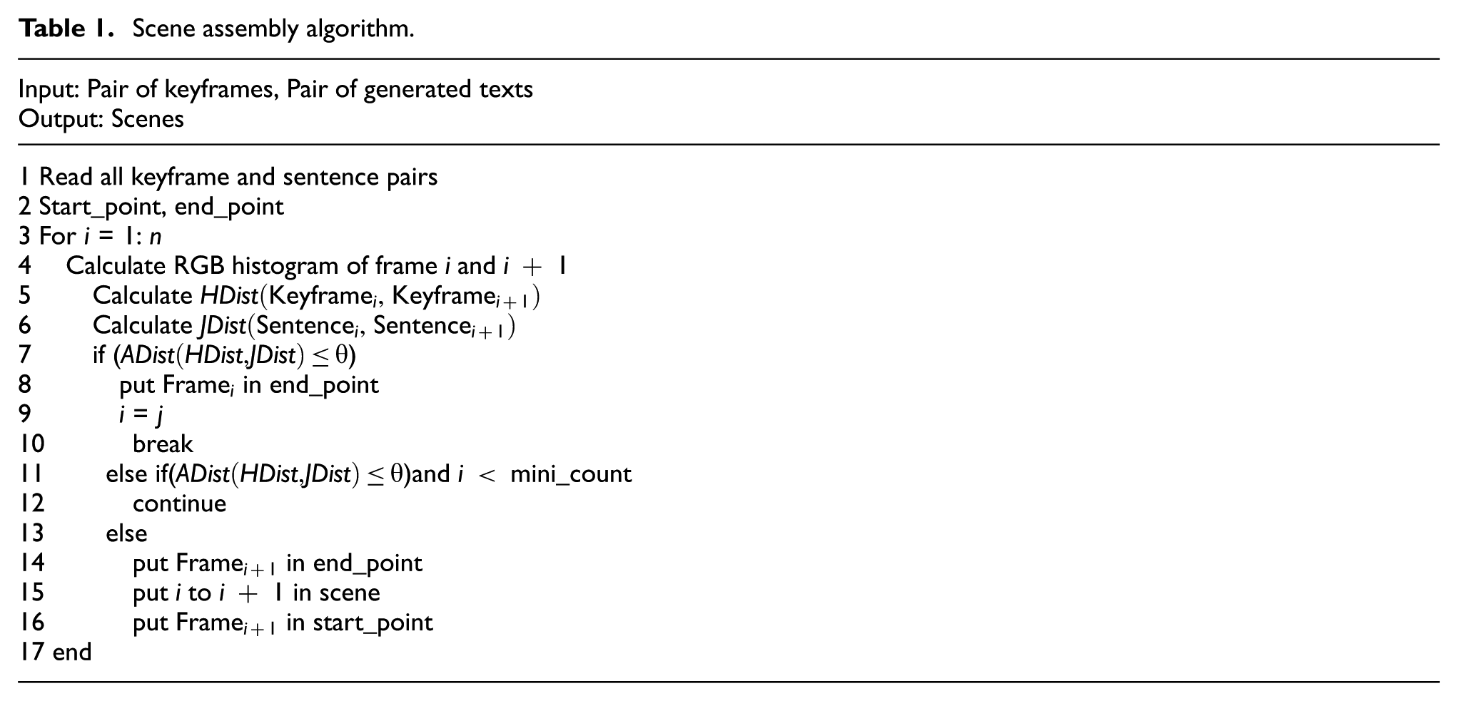
Where n is the total number of keyframes; mini_count is the minimum number of shots to form a scene, which in this article will be eight, as proposed in Krizhevsky et al. [24]. θ is the fixed threshold value that determines the scene. ADist is the equation where the similarity calculations of the histogram and texts are finally calculated, as presented in equation (16)

ADist (HDist, JDist) = α * JDist + (1 - α) * HDist

(16)

where α is the threshold value between 0 and 1 that determines whether to add more weight between histogram similarity or text similarity. Therefore, ADist will conclusively have the value of 1 if the two keyframes’ colour and meaning are similar and will be 0 if they are not similar. In Algorithm 1 (see Table 1), the scene is finally divided according to the value of θ.

4. Experiments

To evaluate the proposed approach, in this section, we test DeepSSS on a TRECVid 2016 data set. The CPU model of the computer used for the experiment was the Intel Core i7-6700; the RAM capacity was 32 G; the GPU was the NVidia GeForce 1080 model; and the operating system was Ubuntu version 16.04. The programming language was python 3.5, and we used the deep-learning library of TensorFlow 1.0.

4.1. Data sets

In this article, for a more objective and accurate performance evaluation of the DeepSSS, two data sets have been used: MS COCO [30] and TRECVid 2016 [31]. The MS COCO data set was used to train the proposed model’s extraction of semantic information from keyframes. The data used consisted of 82,783 training image sets, 40,504 validation image sets and 40,775 test image sets. Each image had five sentences describing it.

The TRECVid 2016 [31,32] data set was a publicly available evaluation data set for video-content-based analysis and retrieval, and has been consistently updated since 2009. The data set provides various types of multimedia data sets. In this article, we used the IACC.3 data set of 2016. The data set consists of approximately 4600 Internet archive videos of 144 GB with a length of 600 h in MPEG-4 format. The videos lengths were between 6.5 and 9.5 min, with an average of 7.8 min. Because of lack of time and the massive size of the data set, for this experiment, we randomly extracted only 10 videos from the data set for the evaluation of DeepSSS.

4.2. Evaluation metrics

We evaluated DeepSSS based on two tasks: (1) accuracy of shot boundary detection and keyframe extraction and (2) accuracy of semantic scene segmentation.

First, the shot boundary detection and keyframe extraction were evaluated through recall, precision and the F-measure metric as shown in equation (17)

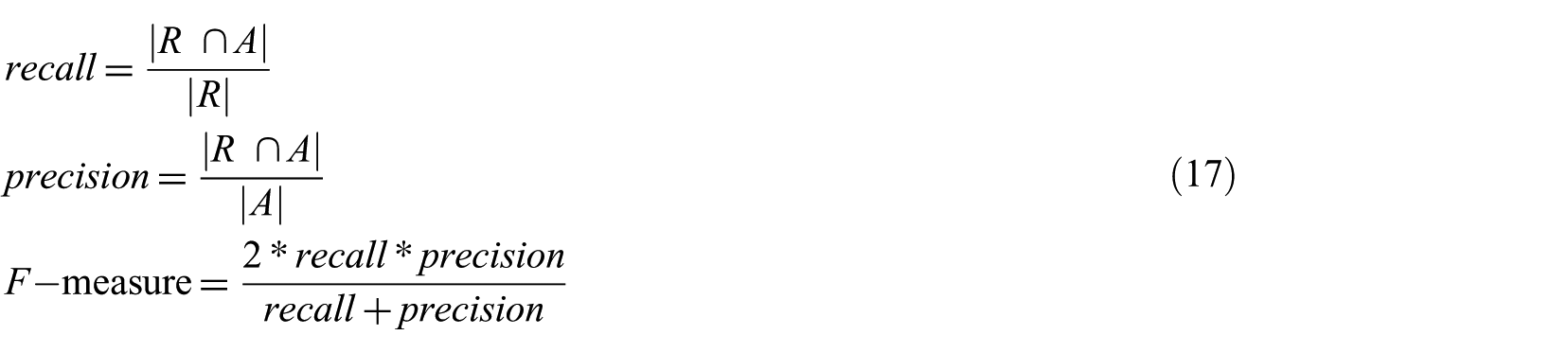
\begin{matrix} recall = \frac{| R \cap A |}{| R |} \\ precision = \frac{| R \cap A |}{| A |} \\ F - measure = \frac{2 * recall * precision}{recall + precision} \end{matrix}

(17)

A is the set of automatically detected shot boundaries and keyframes from the models and R is from the answer sets; ‘recall’ is the percentage of the correct answers (shot boundaries and keyframes) that the model automatically detected from the whole answer set; ‘precision’ is the percentage of correct answers the model automatically detected out of all the shot boundaries and keyframes the model automatically detected. Both of these values, recall and precision, are in a trade-off relationship. Therefore, the F-measure combines the recall and precision value into a single value. These three values, recall, precision and F-measure, are often used in other shot boundary detection and keyframe extraction studies to verify the accuracy of a model, which led to our decision to use the very same verification method to establish the superiority of the proposed model in this article.

Second, the semantic scene segmentation has been evaluated by coverage and overflow [33] as in equation (18)

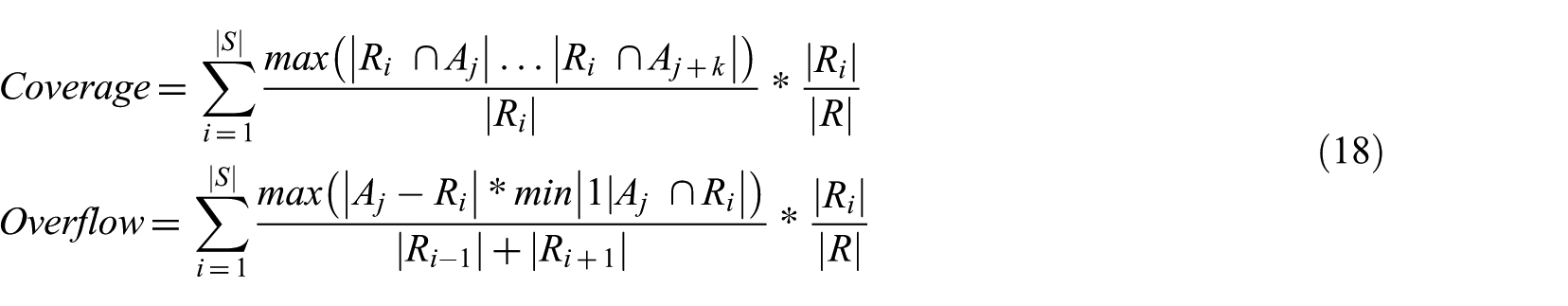
\begin{matrix} Coverage = \sum_{i = 1}^{| S |} \frac{\max (| R_{i} \cap A_{j} | \dots | R_{i} \cap A_{j + k} |)}{| R_{i} |} * \frac{| R_{i} |}{| R |} \\ Overflow = \sum_{i = 1}^{| S |} \frac{\max (| A_{j} - R_{i} | * \min | 1 | A_{j} \cap R_{i} |)}{| R_{i - 1} | + | R_{i + 1} |} * \frac{| R_{i} |}{| R |} \end{matrix}

(18)

where A is a set of automatically detected scenes and R is the answer set. S refers to the total number of scenes. Coverage refers to how much the automatically detected scenes cover the scenes of the answer set. The closer the value is to 1, the better the performance. Overflow refers to how much the automatically detected scenes deviate from the scenes of the answer set. The closer the value is to 0, the better the performance.

4.3. Result on semantic scene segmentation

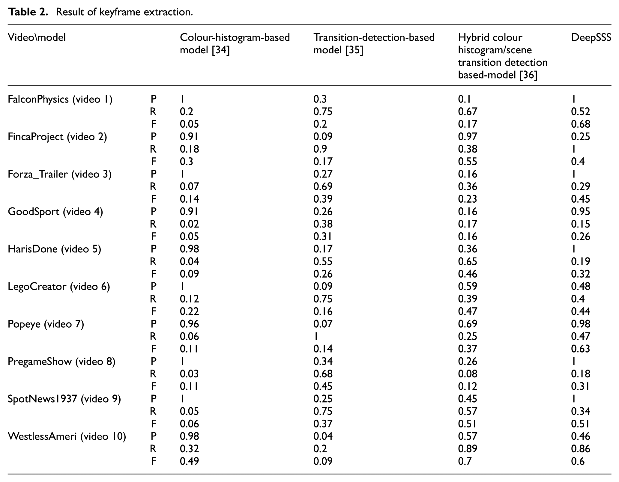
In this article, to evaluate scene segmentation, we have compared the colour-histogram-based model [34], scene-transition (fades/cut in/outs to blacks) detection-based model [35] and the hybrid model based on both colour histogram and scene-transition detection [36]. We have used 10 random Internet archive videos from the TRECVid 2016 data set. Table 2 compares the keyframe extraction results of the above three models and DeepSSS. In Table 2, P refers to Precision, R to Recall and F refers to F-measure. Experimental results show that the colour-histogram-based model shows a very low recall value, compared with its exceedingly high precision value, because it extracted an excessive number of keyframes. Eventually, it extracted a keyframe only when a change was detected in the colour histogram and therefore showed poor results. For the transition-detection-based model, although it had the highest recall rate, its precision was relatively too small, indicating low performance. The hybrid model had almost identical precision and recall values and was more stable than the other two approaches.

Table 2.

Result of keyframe extraction.

Video\model		Colour-histogram-basedmodel [34]	Transition-detection-basedmodel [35]	Hybrid colourhistogram/scenetransition detectionbased-model [36]	DeepSSS
FalconPhysics (video 1)	P	1	0.3	0.1	1
	R	0.2	0.75	0.67	0.52
	F	0.05	0.2	0.17	0.68
FincaProject (video 2)	P	0.91	0.09	0.97	0.25
	R	0.18	0.9	0.38	1
	F	0.3	0.17	0.55	0.4
Forza_Trailer (video 3)	P	1	0.27	0.16	1
	R	0.07	0.69	0.36	0.29
	F	0.14	0.39	0.23	0.45
GoodSport (video 4)	P	0.91	0.26	0.16	0.95
	R	0.02	0.38	0.17	0.15
	F	0.05	0.31	0.16	0.26
HarisDone (video 5)	P	0.98	0.17	0.36	1
	R	0.04	0.55	0.65	0.19
	F	0.09	0.26	0.46	0.32
LegoCreator (video 6)	P	1	0.09	0.59	0.48
	R	0.12	0.75	0.39	0.4
	F	0.22	0.16	0.47	0.44
Popeye (video 7)	P	0.96	0.07	0.69	0.98
	R	0.06	1	0.25	0.47
	F	0.11	0.14	0.37	0.63
PregameShow (video 8)	P	1	0.34	0.26	1
	R	0.03	0.68	0.08	0.18
	F	0.11	0.45	0.12	0.31
SpotNews1937 (video 9)	P	1	0.25	0.45	1
	R	0.05	0.75	0.57	0.34
	F	0.06	0.37	0.51	0.51
WestlessAmeri (video 10)	P	0.98	0.04	0.57	0.46
	R	0.32	0.2	0.89	0.86
	F	0.49	0.09	0.7	0.6

Although there were minor differences depending on the type or genre of the video, the DeepSSS, on average, performed better in extracting keyframes than did the other models. Figure 4 shows the average values of Precision, Recall and F-measure for each model. Note that DeepSSS’F-measure value is the highest. However, the overall low value of Recall indicates that there is room for improvements.

Figure 4.

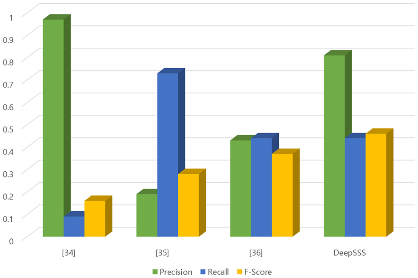
Result of 10 videos’ average evaluation values.

We intended to use the TRECVid 2016 data sets to evaluate the DeepSSS’ semantic scene segmentation. However, according to our research, a data set for semantic scene segmentation does not exist yet. Therefore, the TRECVid video data was manually segmented into scenes and used as an answer set. The answer set was created by test subjects. A dozen average adults of both genders were hired to mark the videos in order to segment them semantically. Then, by binding the common parts that most test subjects pointed out as a semantic boundary for a scene, and smoothing around the more uncommon boundaries, the test subjects marked semantic boundaries. Table 3 shows the results of the hybrid model [36] and the semantic scene segmentation of DeepSSS. The hybrid model’s scene segmentation was the result of using histogram distances, whereas the DeepSSS is a hybrid method, using both histogram distance and sentence similarity for scene segmentation.

Table 3.

Result of semantic scene segmentation.

Video\model		Hybrid colour histogram/scene transition detection based-model [36]	DeepSSS
FalconPhysics (video 1)	Coverage	0.37	0.6
	Overflow	0.62	0.32
FincaProject (video 2)	Coverage	0.31	0.75
	Overflow	0.67	0.19
Forza_Trailer (video 3)	Coverage	0.21	0.62
	Overflow	0.77	0.31
GoodSport (video 4)	Coverage	0.24	0.63
	Overflow	0.71	0.29
HarisDone (video 5)	Coverage	0.18	0.75
	Overflow	0.74	0.22
LegoCreator (video 6)	Coverage	0.34	0.66
	Overflow	0.61	0.31
Popeye (video 7)	Coverage	0.33	0.65
	Overflow	0.59	0.27
PregameShow (video 8)	Coverage	0.27	0.65
	Overflow	0.58	0.3
SpotNews1937 (video 9)	Coverage	0.3	0.69
	Overflow	0.68	0.28
WestlessAmeri (video 10)	Coverage	0.38	0.61
	Overflow	0.57	0.23

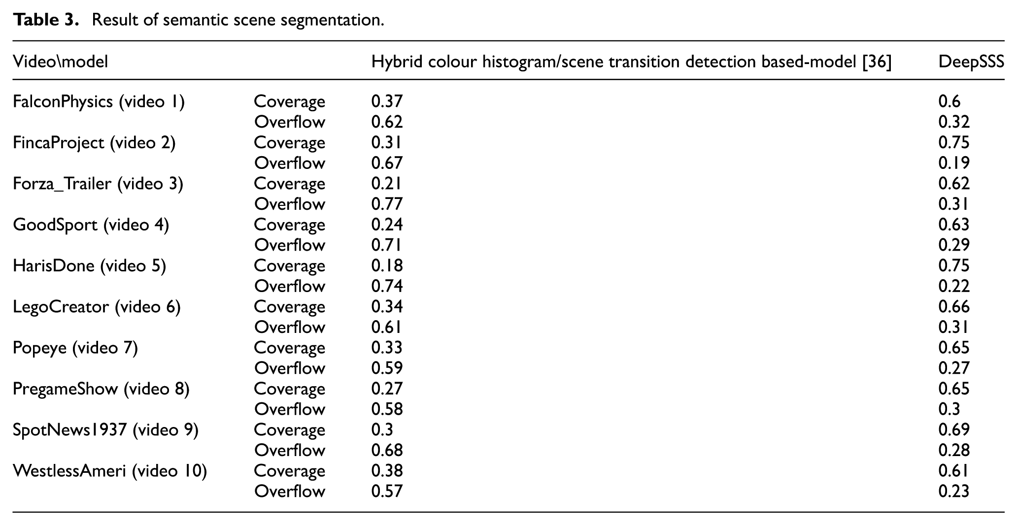
The experimental results show that for the hybrid model [35], the coverage was so low (average 0.29) that it is clear no semantic scene segmentation has taken place. However, DeepSSS’ mean coverage average of 0.66 shows that it can segment video into scenes in a way that resembles how a human would do it, proving the validity of the hypothesis established earlier in this article.

5. Discussion and conclusion

In this article, we have proposed a Deep-learning Semantic-based Scene-segmentation model (called DeepSSS). The DeepSSS performs shot boundary detection by comparing colour histograms, performing maximum-entropy-applied keyframe extraction, and for semantic analysis, DeepSSS generated semantic text descriptions from the keyframe using deep learning and by comparing each keyframe attributed it to scene segmentation. The scene segmentation was performed by a hybrid method of using both histogram distance and text description similarity values. By applying DeepSSS to data sets from MS COCO for caption generation and evaluating its semantic scene-segmentation task results with the data sets from TRECVid 2016, we demonstrated quantitatively that DeepSSS outperforms other existing scene-segmentation methods that uses shot boundary detection and keyframes.

The experiment revealed that, because there is a difference in the histogram similarity calculation, there is no significant improvement over the results of previous methods. In other words, the more the shots composing the video are changed, and the more spectacular the scene, the lower the performance.

This is the limitation of methods that merely use colour histograms, because the colour value of a simple image always stays at a certain level of detection of the shot. For performing scene segmentation using this method, the colour histogram’s limits are inherent; scenes cannot be analysed semantically, and the best that can be achieved is scene segmentation by simple colour value. Nonetheless, unlike previous scene-segmentation methods, DeepSSS benefits from high-level features, aside from low-level features, offering better performances and thereby achieving results similar to those of human segmentation. This demonstrates that high-level feature-based analysis uses a process similar to that of a human being.

In the future, full video-based scene detection rather than keyframe-based detection should be considered in order to achieve better performance, posing the additional challenge of solving the problem of the volume of calculation required when using full video. Moreover, more data sets are required to conduct more comprehensive experimental studies on scene segmentation. In this study, since there were not many data sets for the scene segmentation, detailed comparison experiments across a variety of data sets were difficult. To overcome this limitation, the TRECVid 2016 video data set was constructed through human input. Consequently, it would be better to test DeepSSS with more data sets in the future.

Footnotes

Declaration of conflicting interests

The author(s) declared no potential conflicts of interest with respect to the research, authorship and/or publication of this article.

Funding

This work was supported by the Ministry of Culture, Sport and Tourism (MCST) and Korea Creative Content Agency (KOCCA) in the Culture Technology (CT) Research & Development Program 2018 (No. R2016030031).

References

Enser

The evolution of visual information retrieval. J Inf Sci 2008; 34(4): 531–546.

Nemati

Naghsh-Nilchi

AR.

Incorporating social media comments in affective video retrieval. J Inf Sci 2016; 42(4): 524–538.

Kim

Lee

Han

, et al. Exploring characteristics of video consuming behaviour in different social media using K-pop videos. J Inf Sci 2014; 40(6): 806–822.

Albanese

Molinaro

Persia

, et al. Discovering the top-k unexplained sequences in time-stamped observation data. IEEE T Knowl Data En 2014; 26(3): 577–594.

Albertson

Examining feedback in interactive video retrieval. J Inf Sci 2012; 38(6): 501–511.

Wactlar

HD.

The challenges of continuous capture, contemporaneous analysis and customized summarization of video content, 2001, https://pdfs.semanticscholar.org/9de4/0d04535729707aaad62410ed8a6b2fdfc25e.pdf

Hooshyar

Yousefi

Lim

Data-driven approaches to game player modeling: a systematic literature review. ACM Comput Surv 2018; 50(6): 90.

Hooshyar

Park

, et al. Early diagnosis of dementia from clinical data by machine learning techniques. Appl Sci 2017; 7(7): 651.

Yun

Hooshyar

, et al. Developing a hybrid collaborative filtering recommendation system with opinion mining on purchase review. J Inf Sci 2018; 44(3): 331–344.

10.

Naphide

Huang

TS.

A probabilistic framework for semantic video indexing, filtering, and retrieval. IEEE T Multimedia 2011; 3(1): 141–151.

11.

Del Fabro

Böszörmenyi

. State-of-the-art and future challenges in video scene detection: a survey. Multimedia Syst 2013; 19(5): 427–454.

12.

Ioannidis

Chasanis

Likas

Weighted multi-view key-frame extraction. Pattern Recogn Lett 2016; 72: 52–61.

13.

Rasheed

Shah

Scene detection in Hollywood movies and TV shows. In: Proceedings of the 2003 IEEE computer society conference on computer vision and pattern recognition, Madison, WI, 18–20 June 2003, vol. 2, pp. II–343. New York: IEEE.

14.

Rasheed

Shah

. A graph theoretic approach for scene detection in produced videos. In: Multimedia information retrieval workshop, 2003, http://crcv.ucf.edu/papers/Rasheed_sigir03.pdf

15.

Shi

Malik

Normalized cuts and image segmentation. IEEE T Pattern Anal 2000; 22(8): 888–905.

16.

Zhai

Shah

. A general framework for temporal video scene segmentation. In: 2005 tenth IEEE international conference on computer vision (ICCV 2005), Beijing, China, 17–21 October 2005, vol. 2, pp. 1111–1116. New York: IEEE.

17.

Mei

Hua

, et al. EMS: energy minimization based video. In: 2007 IEEE international conference on multimedia and expo, Beijing, China, 2–5 July 2007, pp. 520–523. New York: IEEE.

18.

Deselaers

Keysers

Ney

Features for image retrieval: an experimental comparison. Inform Retrieval 2008; 11(2): 77–107.

19.

Deselaers

Keysers

Ney

. Features for image retrieval: a quantitative comparison. In: Joint pattern recognition symposium, Tübingen, 30 August–1 September 2004, pp. 228–236. Berlin; Heidelberg: Springer.

20.

Zhou

, et al. Unsupervised, efficient and scalable key-frame selection for automatic summarization of surveillance videos. Multimed Tools Appl 2017; 76(5): 6309–6331.

21.

Yeo

Zhu

Sun

, et al. A framework for sub-window shot detection. In: Proceedings of the 11th international multimedia modelling conference 2005 (MMM 2005), Melbourne, VIC, Australia, 12–14 January 2005, pp. 84–91. New York: IEEE.

22.

Koprinska

Carrato

Temporal video segmentation: a survey. Signal Process: Image 2001; 16(5): 477–500.

23.

Cooper

Liu

Rieffel

Video segmentation via temporal pattern classification. IEEE T Multimedia 2007; 9(3): 610–618.

24.

Krizhevsky

Sutskever

Hinton

GE.

ImageNet classification with deep convolutional neural networks. In: Advances in neural information processing systems, Lake Tahoe, NV, 3–6 December 2012, pp. 1097–1105. New York: Curran Associates.

25.

Vinyals

Toshev

Bengio

, et al. Show and tell: lessons learned from the 2015 MS COCO image captioning challenge. IEEE T Pattern Anal 2016; 39(4): 652–663.

26.

Wang

Yang

Bartz

, et al. Image captioning with deep bidirectional LSTMs. In: Proceedings of the 2016 ACM on multimedia conference, Amsterdam, 15–19 October 2016, pp. 988–997. New York: ACM.

27.

Cho

van Merrienboer

Gulcehre

, et al. Learning phrase representations using RNN encoder-decoder for statistical machine translation, 2014, https://arxiv.org/abs/1406.1078

28.

Graves

Mohamed

Hinton

Speech recognition with deep recurrent neural networks. In: 2013 IEEE international conference on acoustics, speech and signal processing (ICASSP), Vancouver, BC, Canada, 26–31 May 2013, pp. 6645–6649. New York: IEEE.

29.

Sutskever

Vinyals

QV.

Sequence to sequence learning with neural networks. In: Advances in neural information processing systems, Montreal, QC, Canada, 08–13 December 2014, pp. 3104–3112. Cambridge, MA: MIT Press.

30.

Lin

Maire

Belongie

, et al. Microsoft coco: common objects in context. In: European conference on computer vision, Zürich, 6–12 September 2014, pp. 740–755. Cham: Springer.

31.

Awad

Fiscus

Michel

, et al. TRECVid 2016: evaluating video search, video event detection, localization, and hyperlinking. In: Proceedings of TRECVid 2016, Gaithersburg, MD, 14–16 November 2016.

32.

Thornley

McLoughlin

Johnson

, et al. A bibliometric study of video retrieval evaluation benchmarking (TRECVid): a methodological analysis. J Inf Sci 2011; 37(6): 577–593.

33.

Vendrig

Worring

Systematic evaluation of logical story unit segmentation. IEEE T Multimedia 2002; 4(4): 492–499.

34.

Hoi

SCH

Wong

LLS

Lyu

Chinese university of hongkong at trecvid 2006: Shot boundary detection and video search. In: TRECVid 2006 Workshop, Gaithersburg, Maryland, NIST, 2006. pp. 76–86.

35.

Porter

SV.

Video segmentation and indexing using motion estimation. PhD Thesis, University of Bristol, Bristol, 2004.

36.

Huo

Wang

. Effective algorithms for video shot and scene boundaries detection. In: 2016 IEEE/ACIS 15th international conference on computer and information science (ICIS), Okayama, Japan, 26–29 June 2016, pp. 1–6. New York: IEEE.