Does Earning More Than Your Spouse Increase Your Financial Satisfaction? A Comparison of Men and Women in the United States,1982 to 2012

Abstract

Scholars have argued that both husbands and wives are less satisfied if wives outearn their husbands because this violates the norms of the male breadwinner model. Some scholars find support for this hypothesis when studying the division of household work, marital dissolution, or depression, but other scholars do not find clear evidence. This article adds to this literature by asking how people’s roles in bringing money into the household (as a primary or secondary earner) affect how they feel about that money itself. Analysis of decades of U.S. data finds a clear and consistent result: individuals—whether men or women, whether committed to the male breadwinner model or not—are all more satisfied with their family’s financial situation when they earn more than their spouse. Here, generic social psychological processes (like relative deprivation) appear to trump even powerful worldviews, like the male breadwinner model.

Keywords

relative deprivation relative income financial satisfaction male breadwinner model

Introduction

Scholars have been deeply interested in the consequences of married women’s increased labor market participation over the past 50 years for all members of the household, including husbands, children, and wives themselves (Blau & Kahn, 2007; Blossfeld & Drobnic, 2001; Inglehart & Norris, 2003). Building off of this literature, researchers have increasingly examined the role that earning more than one’s spouse has on many outcomes, like the division of household labor (Bittman, England, Sayer, Folbre, & Matheson, 2003), negotiating purchasing decisions (Nyman, 1999; Ward-Batts, 2008), and marital dissolution (Sayer, England, Allison, & Kangas, 2011). This concern over spouses’ relative incomes is all the more pressing, now that in the United States, the percentage of wives earning more than their husbands (as long as they both earn some income) has risen from 18% in 1987 to 29% in 2012 (U.S. Department of Labor, Bureau of Labor Statistics, 2014).

Researcher expectations have been grounded primarily in the idea that the male breadwinner model—with men being the primary (or exclusive) provider and women being responsible for children and the household (Cunningham, 2008)—was normative for all couples. Researchers looked for evidence that as wives earned more, strains on couples would increase, thereby destabilizing the marriage (Sayer et al., 2011) or precipitating coping behaviors from both parties to preserve traditional gender roles (Bittman et al., 2003; Pierce, Dahl, & Nielsen, 2013). Overall, the evidence has been mixed, with some effects observed on subsets of couples (e.g., on divorce, see Sayer et al., 2011; on coping behaviors, see Sullivan, 2011a, 2011b).

Besides the changes in behavior studied above, researchers have also examined how relative income within the couple may affect individuals’ subjective well-being, whether their mental health (Crowley, 1998), global happiness (Gong, 2007), or satisfaction with their marriage (Gong, 2007; Gray-Little & Burks, 1983). Here, too, results have been somewhat inconclusive. One additional dimension of subjective well-being that has not received much consideration, at least in the United States, is satisfaction with one’s financial situation. It should be studied further, however, because it has been strongly linked with individuals’ overall levels of well-being and welfare (Easterlin, 2006), “depression (St. John et al., 2006), . . . perceived health (Cairney, 2000), workplace productivity (Epstein & Ward, 2006), . . . mortality (Blazer et al., 2005)” (DePianto, 2011, p. 774), food consumption (Briers & Laporte, 2013), and gambling and lottery playing (Callan, Ellard, Shead, & Hodgins, 2008).

Given the mixed record of finding relative income effects outlined above, why analyze yet another potential outcome? Satisfaction domain theory (Easterlin & Sawangfa, 2009; Lam & Rotolo, 2001) predicts that relative spousal income should have a strong and clear effect on an individual’s financial satisfaction because, not surprisingly, income is highly salient to the evaluation of one’s finances. This theory also predicts, however, that income (relative or absolute) may not affect satisfaction in other domains of life, like family life or marriage, which might partly explain null results from earlier studies (e.g., Gong, 2007; Rojas, 2007). As Easterlin (2003) notes, “Social comparison affect[s] utility less in the nonpecuniary than pecuniary domains” (p. 11176), meaning relative income will affect people’s opinions about their income situation but may not spill over into other domains. Furthermore, an extensive experimental literature finds “even subtle reminders of money” lead subjects to become quite distracted about anything other than money (Vohs, Mead, & Goode, 2008, p. 208). We should expect, therefore, that people’s different roles in bringing money into the household, either as a primary or secondary earner, will influence how they feel about that money, when they are asked about it.

Recognizing its direct relation to relative spousal income, some scholars have begun to study financial satisfaction, but mostly in Europe (Ahn, Ateca-Amestoy, & Ugidos, 2014; Bonke, 2008; Bonke & Browning, 2009; Rojas, 2007). The United States is a natural site, however, to study the role of relative income among spouses on financial satisfaction because here achieving a high income is a particularly important value (DiPrete, 2007; Verbakel & DiPrete, 2008); and so, income differences within the family may be more visible (and more crucial) in the United States than in most European countries, with more communitarian and egalitarian traditions (Bonke, 2008). The United States also has above-average levels of female participation in the labor force, especially full-time employment (Cotter, England, & Hermsen, 2009, as cited in Sayer et al., 2011); and consequently, many couples have two full-time working members, and this produces a strong possibility that women can earn as much as, if not more than, men. This article, therefore, focuses on the United States.

Last, this article directly confronts the male breadwinner ideology in affecting people’s satisfaction with their financial situation. A major limitation of previous research is that it has relied on an unarticulated premise that the traditional male breadwinner model is the standard against which all couples compare their own income situation, but this has not been tested. Occasionally, researchers compare their results in Northern Europe, which is seen as less tied to the male breadwinner model, with those in Southern Europe, which is thought more traditionalist (Bonke, 2008). Not only have the results of these broad comparisons not been fully consistent with theoretical expectations but this type of approach is also too reliant on stylized understandings of the differences between welfare state regimes, without acknowledging tremendous individual heterogeneity in the adoption of a male breadwinner perspective within countries. This article will ascertain each person’s commitment to traditional gender roles and then incorporate it directly into the analysis.

Against this backdrop, this article seeks to answer the following questions. First, are husbands more financially satisfied when they earn more than their wives, but wives less satisfied when they earn more, as predicted by the male breadwinner model? Second, is the relationship between financial satisfaction and relative income dependent not just on being a man or a women but also on one’s level of gender traditionalism? We analyze decades of public opinion data from the United States to answer these questions.

Male Breadwinner Model, Gender Display, and Gender Deviance Neutralization

For most of the past century in the United States, the male breadwinner model was the dominant ideal (England, 2010; Sayer et al., 2011). This model for family relations is premised on specialization between husbands and wives, with men responsible for bringing money into the household through wage work and women responsible for the workings of the home, including caring for children (Cunningham, 2008). This model was structurally embedded in legal arrangements like Social Security payment schemes that favor male workers over female ones (Pascall & Lewis, 2004). This model, though never close to being realized by many families, nonetheless still holds sway over the public’s evaluations of marriage, work, and family (Pascall & Lewis, 2004).

Scholars have tried to determine how relative income among spouses relates to this male breadwinner model in our time. Spouses are aware of what is typically expected of them as husbands and wives. Some spouses who deviate from the male breadwinner model in earnings might attempt to compensate with gender-normative roles in other parts of family life. If husbands are not the main provider, for instance, they might look for ways to display traditional masculinity by refusing to do household tasks (e.g., laundry, cooking, child care), even if they have time to do them (Bittman et al., 2003), or by initiating an affair (Munsch, 2012), or by maintaining sexual prowess by taking erectile dysfunction medication (Pierce et al., 2013). This is part of a gender display strategy or “doing gender” (West & Zimmerman, 1987). If men are unable to be the primary provider and the gender role ambiguity is unsatisfactory, they may display higher levels of depression (Crowley, 1998; Pierce et al., 2013) and perhaps commit higher rates of violence toward women (Atkinson, Greenstein, & Lang, 2005).

Likewise, if wives earn more than their husbands, they may try to minimize this reality, by performing the role of stay-at-home wives, spending a disproportionate amount of their time on household tasks (Bittman et al., 2003; Greenstein, 2000), or by not asserting their full bargaining power in household decisions (Atkinson & Boles, 1984; Lundberg, Pollak, & Wales, 1997; McRae, 1987). This is part of a gender deviance neutralization strategy (Simister, 2013). If women earn more than their spouse and find this position untenable, they may be more likely to depart the marriage (for a review on this, see Sayer et al., 2011) or medicate themselves for anxiety and insomnia (Pierce et al., 2013).

Some empirical evidence concerning relative income and financial satisfaction already points toward a dynamic consistent with the male breadwinner model. In the most sophisticated study to date, Bonke (2008) studies 11 European countries, examining changes in individuals’ financial satisfaction, as the share of income that the wife contributes to the household grows. He occasionally finds that men’s financial satisfaction declines as their wives earn more (e.g., in Belgium and Luxembourg), which is what the male breadwinner model would predict. Additionally, Ahn et al. (2014) find that in Spain, men are more financially satisfied if they earn more than their wives.

The theoretical expectations above would lead to the following hypothesis:

Hypothesis 1a: Husbands will be more financially satisfied when they earn more than their wives, but wives will be less satisfied when they earn more.

Social Comparison, Relative Income, and Spouse as a Reference Group

Other theoretical perspectives, however, generate alternative hypotheses. Like the gender display and gender deviance neutralization perspectives, the social comparison perspective (Walker & Smith, 2002) starts from the fact that one spouse knows she or he makes more than the other. But unlike those other theories, the social comparison perspective argues that gender norms do not define how individuals respond to their relatively superior income positions. Instead, social comparison is ubiquitous and inevitable (Clark, Frijters, & Shields, 2008; Easterlin, 1995; Layard, 2006; Turley, 2002), and it occurs when people mainly judge their situation not based on the absolute (or objective) value of the things they have, but on the relative value of those things, compared with what people, whom they consider their equals, have.

The original instance of social comparison was “relative deprivation,” coined by Stouffer, Suchman, DeVinney, Star, and Williams (1949) to explain some puzzling results of their massive study of the military. For instance, they wondered why African American soldiers stationed in the South were more satisfied than African American soldiers in the North, even though the South was more segregated and hostile to African Americans. This and other “apparent puzzles assumed the wrong referent comparisons. Immediate comparisons . . . were the salient referents” (Pettigrew, 2002, p. 351): African American soldiers compared themselves with those most similar to them and most near to them—that is, civilian African Americans in the region where they were stationed. African American soldiers in the South felt relatively better off, compared with the limited and unjust living conditions of Southern African American civilians, while African American soldiers in the North were comparing themselves unfavorably with the freer and more prosperous African Americans around them. These concepts have been extended many times in the past half century since (Pettigrew, 2002).

For social comparison to operate within couples, however, individuals must consider their spouse a legitimate peer to compare against, and there are reasons to think this happens. Few people are more similar than spouses are to each other (Kalmijn, 1998), which would make them prime candidates for social evaluation. Both exchange theory (Ward-Batts, 2008) and bargaining theory lead us to conclude that spouses utilize their individual resources, like earnings, to ensure that their preferences receive full consideration when household decisions are made (Lundberg et al., 1997; Sayer et al., 2011).

Some empirical evidence exists to support this theory as well, since Bonke (2008) also finds in the Netherlands and Greece, women gain greater financial satisfaction as they earn more.

Based on existing theory and this limited empirical evidence, we could hypothesize that a generic social–psychological processes (like social comparison) will trump the norms of the male breadwinner ideal, meaning:

Hypothesis 1b: Both men and women will report increased financial satisfaction when they earn more than their spouse.

The Pooling Model of Household Production

The social comparison theory is not the only alternative theory to consider. Individuals may not allow their own financial satisfaction to depend on making more than their spouse at all. Spouses may not feel like they are competing against each other but instead feel like they are cooperating. If they are pooling all of their resources, this could mean they are only thinking in terms of their absolute total income, as both the neoclassical household economics (Becker, 1991) and the “marriage as a social institution” (Amato, Booth, Johnson, & Rogers, 2007, as cited in Sayer et al., 2011) theories predict.

This is also what Bonke (2008) found in a large proportion of European countries: null results. Specifically, more than a third of the time (in 8 out of 22 equations he runs), he got null findings for men and/or women in European countries, meaning the financial satisfaction of husbands and/or wives is completely unrelated to how much income the wife contributes. He does not present any overall theory for why he gets null results in certain countries for certain sexes, but this ought to lead us to consider that relative income does not have to matter for couples. Moreover, Rojas (2007) finds that in Mexico, financial satisfaction for both men and women is tied only to total family income, not the amount each spouse contributes, perhaps indicating pooling of all resources.

Based on this reasoning and evidence, we could hypothesize:

Hypothesis 1c: Neither men nor women will report increased financial satisfaction when they earn more than their spouse.

Revisiting the Male Breadwinner Model, Considering Gender Traditionalism

There is one final possibility regarding relative income which the existing literature has not addressed. As mentioned earlier, marriage as an institution is often connected to the traditional male breadwinner model, and researchers frequently appear to conflate being a husband with feeling an obligation to act traditionally masculine and being a wife with needing to act traditionally feminine. This approach is clearly too simplistic and fails to acknowledge the tremendous individual heterogeneity in the adoption of the male breadwinner perspective (for a similar critique concerning domestic abuse, see Atkinson et al., 2005). Moreover, research in masculinities has shown that there is not a singular “masculinity,” and masculinites are subject to change, both individually and collectively (Connell & Messerschmidt, 2005).

Analysts should ascertain each person’s commitment to traditional gender roles, and then incorporate that directly into the analysis, as opposed to simply relying on sex as a proxy for it. To our knowledge, the literature has not tested for this possibility.

Given the above analysis, we would make the following prediction:

Hypothesis 2: Only if they subscribe to traditional gender roles, will husbands be more financially satisfied when they earn more than their wives; and only if wives subscribe to traditional gender roles, will they be less satisfied when they earn more.

Data and Method

Data and Analytic Sample

The data come from the Cumulative General Social Survey (GSS), which has been providing a premiere record of American opinions and behaviors since 1972. For most of its history, the GSS was an almost annual survey of the noninstitutionalized, English-speaking population of the United States who were 18 years or older. It is now conducted every 2 years and interviews Spanish speakers as well. Its response rate is over 70%.

We selected our analytic sample as only full-time working individuals who are married and who have a full-time working spouse. This provides the strongest basis for social comparison since these spouses are equivalent on their work statuses, which should enhance their sense of similarity to each other and bring their incomes closer to each other. Only complete cases were used here as well. Observations were pooled across all the surveys between 1982 and 2012, and this amounts to a minimum of 58 observations to a maximum of 266 observations for individual survey “years.”

Dependent Variable

Our dependent variable is family financial satisfaction, which is an answer to the following question: “We are interested in how people are getting along financially these days. So far as you and your family are concerned, would you say that you are (1) not satisfied at all with your present financial situation (2) more or less satisfied or (3) pretty well satisfied?” (This question wording reflects our reverse-coding on the variable.)

Key Independent Variable

Our main independent variable is a dummy variable for whether the respondent makes more than their spouse (=1), and 0 otherwise.¹ This was calculated by first creating the spouse’s income by subtracting the respondent’s income from the total family income (Hout, 2004; Ligon, 1989).

Creating the spouse’s income in this way could be problematic because it attributes nonlabor income (investment income, gifts, government aid, etc.) to the spouse. This does not appear to be a consequential problem, however, because we are able to compare our created measure of spousal income with separate questions that were asked in isolated years of the GSS about how much money the respondents made relative to their spouses. As Table 1 illustrates, when we place our imputed spousal income into this table, it performs well, showing very similar income differences between the respondents and their spouses. In 1996, our measure produces a median difference in incomes of $9,335 for when respondents say they earn much more than their spouse, while when the respondents say that their spouse earns much more, that median income difference is −$12,687. These numbers are of similar magnitude, though obviously with opposing signs. (Medians were used to better handle skewed income data, especially for some cells with very few observations.) When the respondents say that they earn about the same as their spouse, the difference in their incomes is a median of $1.²

Table 1.

The Calculated Median Difference in Earnings Between Husbands and Wives, Utilizing Our Imputation Method.

	Earnsmor (1988, 1994)			Earnmore (1996)
	Men	Women		All
Husband earns much more	$17,190	−$14,234	I earn much more	$9,335
Husband earns a bit more	$7,640	−$4,824	I earn somewhat more	$3,624
Same income for both	$0	−$1,910	We earn about the same	−$1
Wife earns a bit more	−$7,238	$5,730	My spouse/partner earns somewhat more	−$3,626
Wife earns much more	−$14,475	$13,269	My spouse/partner earns much more	−$12,687
	n = 214	n = 222		n = 223

Note. Both the “Earnsmor” (1988, 1994) variable and the “Earnmore” (1996) variable ask the exact same question: “Who earns more money?” The only difference is who the reference for the answers is.

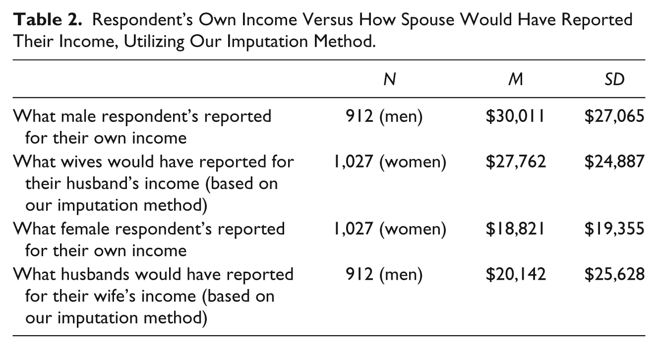
Moreover, based on our methodology, as Table 2 illustrates, for men, they report $30,011 in earnings, on average, while what wives would have reported for their husbands’ incomes (based on our imputation methodology) would be, on average, $27,762. For women, they claim to earn $18,821, on average, while their husbands would have reported their wives’ incomes as $20,142. The actual reported means and our imputed means, therefore, are very similar for each sex, and they are statistically indistinguishable from each other. This indicates that our measure performs quite well.

Table 2.

Respondent’s Own Income Versus How Spouse Would Have Reported Their Income, Utilizing Our Imputation Method.

	N	M	SD
What male respondent’s reported for their own income	912 (men)	$30,011	$27,065
What wives would have reported for their husband’s income (based on our imputation method)	1,027 (women)	$27,762	$24,887
What female respondent’s reported for their own income	1,027 (women)	$18,821	$19,355
What husbands would have reported for their wife’s income (based on our imputation method)	912 (men)	$20,142	$25,628

That said, clearly the lack of a direct measure of spousal income introduces some level of measurement error, but this ought not be problematic, since this error affects both respondents and their spouses equally, meaning that it affects men and women equally as well. If anything, such classic errors-in-variables issues ought to bias any effect sizes toward zero (Wooldridge, 2008), making it harder to detect increases in satisfaction tied to making more than one’s spouse.

Key Control Variable

We created a nontraditional gender ideology measure based on three items asked over the whole of the time series, all with answers ranging from strong agreement to strong disagreement. This scale taps into someone’s commitment to the male breadwinner model. The statements relate to whether (1) it is much better for everyone involved if the man is the achiever outside the home and the woman takes care of the home and family, (2) a working mother cannot establish just as warm and secure a relationship with her children as a mother who does not work, and (3) a preschool child is likely to suffer if his or her mother works (reverse-coded). Greater disagreement with these three statements indicates greater nontraditional gender ideology. We standardized the items and combined them into a scale (Cronbach’s α = .74).

Other Control Variables

Other variables of interest are, and probably most important, the total family income from the past year, logged; sex (male = 0, female = 1); education, measured in total number of years of schooling, top-coded to 20 years; work hours, which refer to the total number of hours worked last week at the person’s job; word score, which is the number of correct answers (out of 10) to vocabulary questions; birth year, which is simply the year the respondent was born, to account for age; survey year, which is the year that survey was administered; an indicator variable for if the respondent was foreign born (=1) or not (=0); an indicator variable for if both of the respondent’s parents were born in the United States (=1) or otherwise (=0); the number of the respondent’s grandparents who were foreign-born; a series of indicators for the respondent’s race, with the reference group being White, and the other choices being African American and any other minority race; the respondent’s answer to a question about how exciting life is, with higher answers indicating increased excitement with life; happiness, with higher scores signaling greater happiness; and an assessment by the interviewer about how cooperative the respondent was with the survey, with higher scores indicating more interest in the survey by the respondent.

Analytic Strategy

Our outcome variable is ordinal in nature, meaning that the categories of opinion are ordered, but it is not appropriate to assume equal spacing between choices. If the opinion variable is assumed to follow a continuous latent distribution, then the appropriate method to employ here is ordinal logistic regression. Based on the proportional odds model, the ordinal logistic regression runs a series of binary logistic regressions, each one based on the probability of being in a lower category versus a higher category at each possible “cut-point” between categories.

Formally, the model is

Log [P (Y \leq j) / P (Y > j)] = α_{j} - β X - β Z, j = 1, 2, \dots, c - 1,

where the log odds are being predicted of being in a higher category than j versus a category as low as, or lower than, j (Agresti & Finlay, 2009); X is a dummy variable if the respondent makes more than his or her spouse; Z is an extensive set of other control variables; and c stands for the number of answer categories. The ordinal logistic assumes that the odds are proportionate across each category jump, but this may not be true; we will note when, and in what way, this assumption is violated. Log odds coefficients are not easy to interpret, and so we have converted all of our resulting logit coefficients into odds ratios (ORs) by simply exponentiating each coefficient for presentation.

Because we have chosen an analytic sample, no sampling weights were applied.

A Final Clarifying Note

In these models, we are not comparing a husband’s satisfaction with the family finances to his own wife’s satisfaction, or vice versa. We do not have the data to do that, and it would answer a different set of questions. What we are doing is comparing equivalent men with each other, but where some men earn more than their wives and where some men earn less than their wives, but they are similar in many other respects, and we are doing the same thing for equivalent women.

Results and Discussion

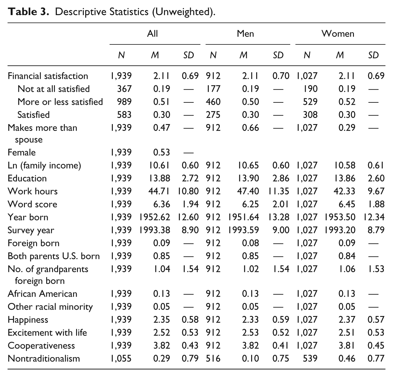
The descriptive statistics found in Table 3 indicate that among married full-time working couples, about half of the respondents are more or less satisfied financially, but approximately 20% are not at all satisfied and 30% are fully satisfied. They generally find life more exciting than not, they are happier than not, and they are almost completely cooperative in their interviews.

Table 3.

Descriptive Statistics (Unweighted).

	All			Men			Women
	N	M	SD	N	M	SD	N	M	SD
Financial satisfaction	1,939	2.11	0.69	912	2.11	0.70	1,027	2.11	0.69
Not at all satisfied	367	0.19	—	177	0.19	—	190	0.19	—
More or less satisfied	989	0.51	—	460	0.50	—	529	0.52	—
Satisfied	583	0.30	—	275	0.30	—	308	0.30	—
Makes more than spouse	1,939	0.47	—	912	0.66	—	1,027	0.29	—
Female	1,939	0.53	—
Ln (family income)	1,939	10.61	0.60	912	10.65	0.60	1,027	10.58	0.61
Education	1,939	13.88	2.72	912	13.90	2.86	1,027	13.86	2.60
Work hours	1,939	44.71	10.80	912	47.40	11.35	1,027	42.33	9.67
Word score	1,939	6.36	1.94	912	6.25	2.01	1,027	6.45	1.88
Year born	1,939	1952.62	12.60	912	1951.64	13.28	1,027	1953.50	12.34
Survey year	1,939	1993.38	8.90	912	1993.59	9.00	1,027	1993.20	8.79
Foreign born	1,939	0.09	—	912	0.08	—	1,027	0.09	—
Both parents U.S. born	1,939	0.85	—	912	0.85	—	1,027	0.84	—
No. of grandparents foreign born	1,939	1.04	1.54	912	1.02	1.54	1,027	1.06	1.53
African American	1,939	0.13	—	912	0.13	—	1,027	0.13	—
Other racial minority	1,939	0.05	—	912	0.05	—	1,027	0.05	—
Happiness	1,939	2.35	0.58	912	2.33	0.59	1,027	2.37	0.57
Excitement with life	1,939	2.52	0.53	912	2.53	0.52	1,027	2.51	0.53
Cooperativeness	1,939	3.82	0.43	912	3.82	0.41	1,027	3.81	0.45
Nontraditionalism	1,055	0.29	0.79	516	0.10	0.75	539	0.46	0.77

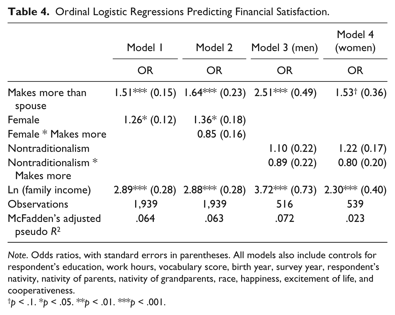
Models 1 and 2 in Table 4 allow us to evaluate our first set of hypotheses. Results from Model 1 support Hypothesis 1b, which claims that making more than one’s spouse, net of gender, increases one’s family financial satisfaction. If individuals make more than their spouse, it increases their odds of being in a higher category of financial satisfaction by 51% (the logit coefficient was 0.41, which when exponentiated, becomes an OR of 1.51), and it is a highly statistically significant result. In fact, after the log of family income and one’s overall level of happiness, whether someone makes more or less than their spouse is the third most important predictor in the model. We also ran models where the “making more” variable was treated continuously, but it did not change our results (full results available on request).

Table 4.

Ordinal Logistic Regressions Predicting Financial Satisfaction.

	Model 1	Model 2	Model 3 (men)	Model 4 (women)
	OR	OR	OR	OR
Makes more than spouse	1.51*** (0.15)	1.64*** (0.23)	2.51*** (0.49)	1.53^† (0.36)
Female	1.26* (0.12)	1.36* (0.18)
Female * Makes more		0.85 (0.16)
Nontraditionalism			1.10 (0.22)	1.22 (0.17)
Nontraditionalism * Makes more			0.89 (0.22)	0.80 (0.20)
Ln (family income)	2.89*** (0.28)	2.88*** (0.28)	3.72*** (0.73)	2.30*** (0.40)
Observations	1,939	1,939	516	539
McFadden’s adjusted pseudo R²	.064	.063	.072	.023

Note. Odds ratios, with standard errors in parentheses. All models also include controls for respondent’s education, work hours, vocabulary score, birth year, survey year, respondent’s nativity, nativity of parents, nativity of grandparents, race, happiness, excitement of life, and cooperativeness.

†

p < .1. *p < .05. **p < .01. ***p < .001.

This means that if there are two equivalent women, and their families both earn the same amount of total money, but one woman makes more than her husband, while the other makes less, then the woman who earns more than her husband is more satisfied with their total family’s income than the woman who earns less, even though it is the exact same amount of total income.³ The same would be true for two men. These results are all the more impressive because of the long list of control variables that make respondents highly equivalent to each other, even being equalized on their overall level of happiness.⁴ The overall fit of this model is moderately strong, with a McFadden’s adjusted pseudo R² of .064.⁵

Perhaps the analysis in Model 1 is too simple and would lead to a premature conclusion. Recall that Hypothesis 1a argued that men and women would react differently to being the main breadwinner, with men being more satisfied and women being less satisfied. Including an interaction between sex and making more money is the appropriate test for this possibility. The results in Model 2 in Table 4 show that the positive effect of being the primary provider appears to work the same way for both men and women because the interaction term does not approach statistical significance. That said, the interaction term is less than 1 (OR = 0.85), which implies a slight tendency for women to gain less satisfaction from making more than their husbands, but this effect is not meaningfully different from zero.

These above results provide evidence against the idea of full pooling of resources in the United States, among full-time working couples (Hypothesis 1c). All people seem to derive more satisfaction from the same amount of absolute income, when they themselves bring the majority of earnings into the household.

It is possible that even though women and men apparently derive the same financial satisfaction from being the primary breadwinner, this is still affected by the person’s overall gender ideology. To test for that, separate models for men and women were run, with an interaction between nontraditional gender ideology and making more money included. Hypothesis 2 is that men who hold more traditional views on gender roles will gain greater satisfaction from being the primary breadwinner, while women who hold traditional views will actually suffer decreased satisfaction as a result of it.

Given our sample of full-time working men and women, it is not surprising that they have higher average scores on the nontraditionalism scale (0.2 for them vs. the full sample average of −0.05), which might appear to make it harder to detect a “male breadwinner effect.” Our sample does not differ that dramatically, however, on this nontraditional ideology measure; see Figure 1 for evidence of this. That chart shows the proportion of people from the full sample and our sample who fall in each of 9 ascending bands of nontraditional ideology. There are fewer lower scores for our sample and more high scores, but the results are not terribly skewed: For instance, 36% of our sample is in the bottom 5 bands, which is not as much as the 49% of the full sample that is in those bands, but is still quite substantial. There is still extensive variation on this measure to test our theories.

Figure 1.

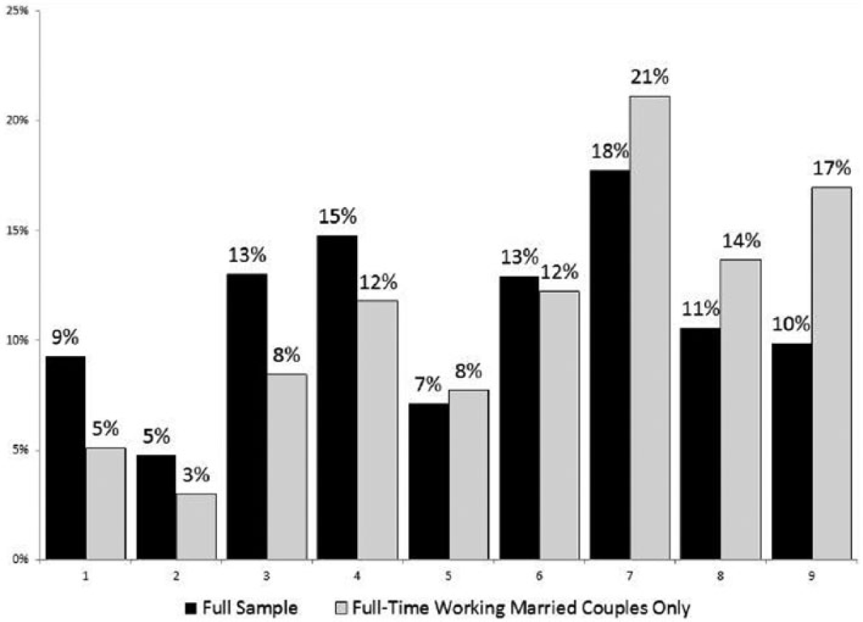
Percentage of people in each band of nontraditional gender ideology, General Social Survey, 1982 to 2012.

For family financial satisfaction, as Model 3 in Table 4 indicates, the interaction of making more money and holding increasingly nontraditional gender opinions for men is not remotely statistically significant and appears to be near zero. This implies that at any level of commitment to traditional masculinity and femininity, men derive the same amount of satisfaction with their family’s financial situation as long as they are earning the bulk of the household’s income. The results for women mirror those of men, as Model 4 indicates, a statistically insignificant interaction term again. If anything, since the interaction term is less than 1 (OR = 0.80), this would imply that contrary to expectations, as women become more feminist in their gender ideology, they actually derive less pleasure from their breadwinner status, compared with how traditional women would feel; but again, the result is not statistically significant.

Robustness Checks

There are a series of additional questions that the above analysis brings to mind, which we ought to consider.

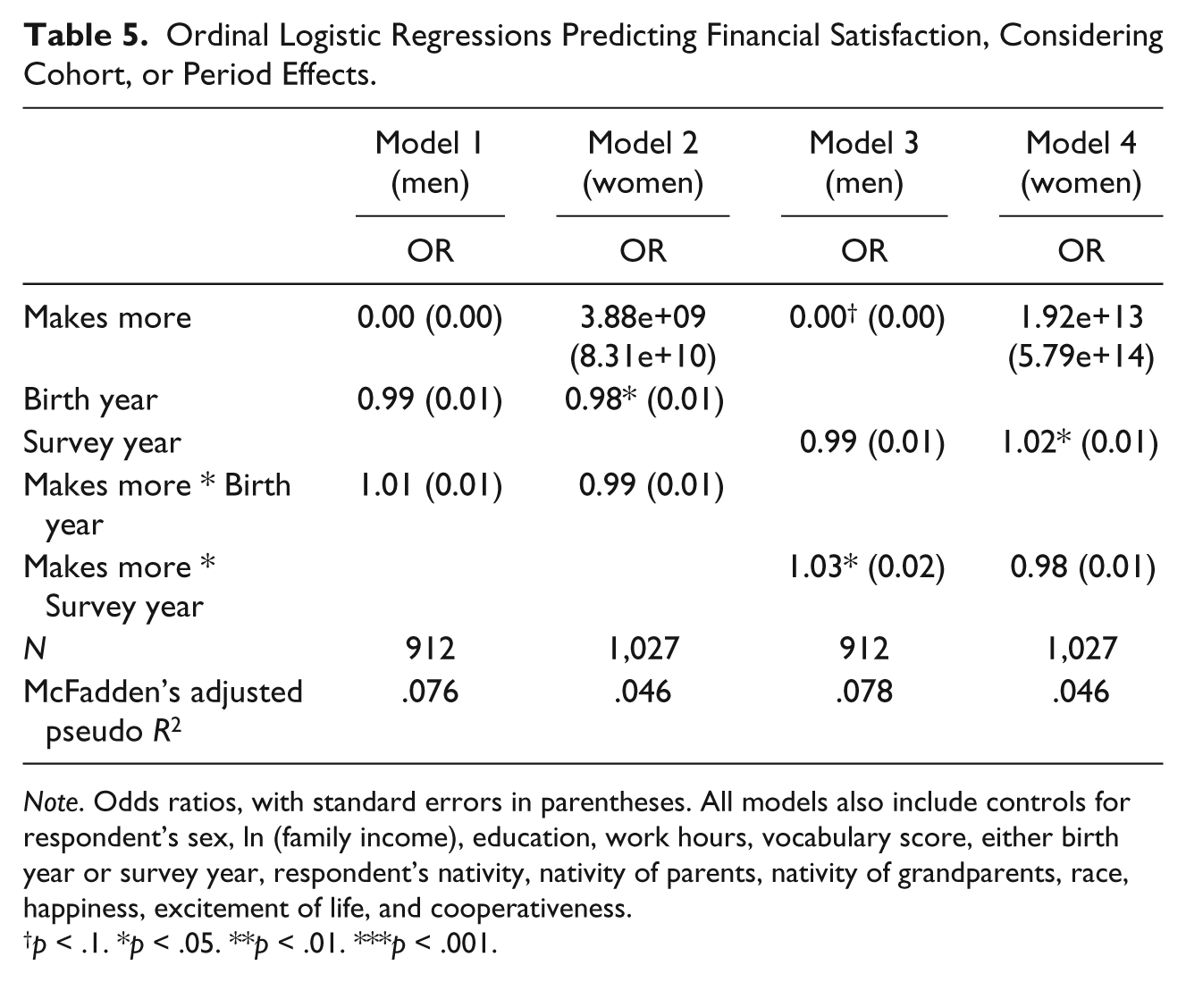
Research Question 1: Has this positive relationship between earning more and financial satisfaction changed across time or for more recent cohorts?

Both gender norms and economic values have changed over the past 40 years, both due to period effects and cohort effects (Inglehart & Norris, 2003). Given the previous literature, we would expect that men were more gratified with their higher earnings prior to the rise of the women’s movement, either as a period effect or a cohort effect—and vice versa for women. As Table 5 shows, there is not much evidence of time variation in this “earning more” effect. Specifically, for both men and women, the interactions on making more money and (linear) birth year are statistically insignificant, indicating that newer cohorts are not feeling differently about making more money. For women, the interaction on making more and (linear) time is also statistically insignificant.⁶ For men, in more recent years, they have been increasing their financial satisfaction more rapidly when they have been making more money than their spouses (OR = 1.03, p < .05), but this is the opposite of what we had hypothesized and the effect size is also quite small.

Research Question 2: Do spouses compare their hourly wages with each other instead of their total annual salaries?

Table 5.

Ordinal Logistic Regressions Predicting Financial Satisfaction, Considering Cohort, or Period Effects.

	Model 1 (men)	Model 2 (women)	Model 3 (men)	Model 4 (women)
	OR	OR	OR	OR
Makes more	0.00 (0.00)	3.88e+09 (8.31e+10)	0.00^† (0.00)	1.92e+13 (5.79e+14)
Birth year	0.99 (0.01)	0.98* (0.01)
Survey year			0.99 (0.01)	1.02* (0.01)
Makes more * Birth year	1.01 (0.01)	0.99 (0.01)
Makes more * Survey year			1.03* (0.02)	0.98 (0.01)
N	912	1,027	912	1,027
McFadden’s adjusted pseudo R²	.076	.046	.078	.046

Note. Odds ratios, with standard errors in parentheses. All models also include controls for respondent’s sex, ln (family income), education, work hours, vocabulary score, either birth year or survey year, respondent’s nativity, nativity of parents, nativity of grandparents, race, happiness, excitement of life, and cooperativeness.

†

p < .1. *p < .05. **p < .01. ***p < .001.

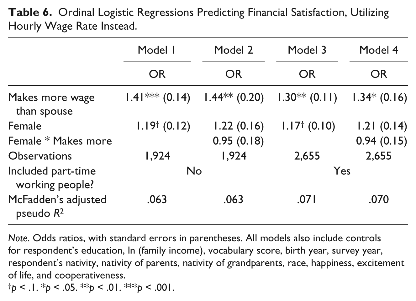
There is a question about what the relevant income comparison should be. Hourly wage is also relevant because spouses could compare their relative hourly wages instead of their relative annual salary (Voydanoff, 1988). When a measure of hourly wage⁷ is used instead, the results are largely the same as for annual salary, though they are somewhat attenuated (in Table 6, Model 1, the OR on making more money using hourly wages = 1.41, p < .001, vs. OR = 1.51, for the original measure using annual salaries). Using a measure of hourly wage also allows us to include people who only work part-time as well as full-time, and when we do that in Model 3 of Table 6, the results are still largely the same as before (OR = 1.30, p < .01).

Research Question 3: Does earning more than their spouse increase individuals’ satisfaction in other domains of their life, like marriage and family, or does it only apply to financially focused parts of their lives?

Table 6.

Ordinal Logistic Regressions Predicting Financial Satisfaction, Utilizing Hourly Wage Rate Instead.

	Model 1	Model 2	Model 3	Model 4
	OR	OR	OR	OR
Makes more wage than spouse	1.41*** (0.14)	1.44** (0.20)	1.30** (0.11)	1.34* (0.16)
Female	1.19^† (0.12)	1.22 (0.16)	1.17^† (0.10)	1.21 (0.14)
Female * Makes more		0.95 (0.18)		0.94 (0.15)
Observations	1,924	1,924	2,655	2,655
Included part-time working people?	No		Yes
McFadden’s adjusted pseudo R²	.063	.063	.071	.070

Note. Odds ratios, with standard errors in parentheses. All models also include controls for respondent’s education, ln (family income), vocabulary score, birth year, survey year, respondent’s nativity, nativity of parents, nativity of grandparents, race, happiness, excitement of life, and cooperativeness.

†

p < .1. *p < .05. **p < .01. ***p < .001.

We have focused on financial satisfaction because we are looking at the effects of different distributions of earnings within the couple, and financial satisfaction obviously has a strong link with earnings. It is reasonable to ask if the result we have here is unique or if it fits into a larger pattern vis-a-vis other domains of life satisfaction. We reran the model developed for financial satisfaction on a series of other variables.

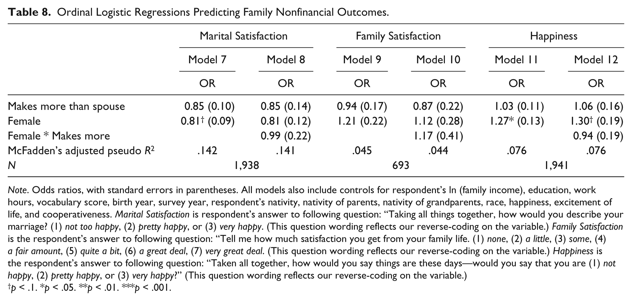
For all of the other financial outcomes, the results are quite similar to that of financial satisfaction. As Table 7 illustrates, both men and women, when they earn more, they are more likely (1) to believe their family is richer than other American families (Model 1: OR = 1.61, p < .001); (2) to believe their financial situation has gotten better (Model 3: OR = 1.21, p < .1); and (3) to say they are more satisfied with the work they do (Model 5: OR = 1.32, p < .01). For nonfinancial outcomes, however, there is no effect associated with earning more money, as Table 8 shows. If they earn more, neither men nor women (1) claim their marriage is more or less happy (Model 7), (2) derive more or less satisfaction from their family life (Model 9), and (3) rate themselves as more or less happy overall (Model 11). We take this as a strong piece of evidence in favor of the domains of satisfaction theory (Easterlin & Sawangfa, 2009).

Table 7.

Ordinal Logistic Regressions Predicting Family Other Financial Outcomes.

	Relative Financial Standing		Improved Financial Situation		Job Satisfaction
	Model 1	Model 2	Model 3	Model 4	Model 5	Model 6
	OR	OR	OR	OR	OR	OR
Makes more than spouse	1.61*** (0.17)	1.85*** (0.28)	1.21^† (0.12)	1.34* (0.19)	1.32** (0.13)	1.20 (0.17)
Female	1.01 (0.11)	1.15 (0.17)	1.00 (0.10)	1.10 (0.15)	1.26* (0.13)	1.16 (0.16)
Female * Makes more		0.76 (0.16)		0.82 (0.16)		1.19 (0.23)
McFadden’s adjusted pseudo R²	.187	.187	.032	.032	.043	.043
N	1,934		1,937		1,937

Note. Odds ratios, with standard errors in parentheses. All models also include controls for respondent’s ln (family income), education, work hours, vocabulary score, birth year, survey year, respondent’s nativity, nativity of parents, nativity of grandparents, race, happiness, excitement of life, and cooperativeness. Relative Financial Standing is the respondent’s answer to the following question: “Compared with American families in general, would you say your family income is (1) far below average, (2) below average, (3) average, (4) above average, or (5) far above average?” Improved Financial Situation is the respondent’s answer to following question: “During the last few years, has your financial situation been getting worse, has it stayed the same, or has it been getting better?” (This question reflects our reordering of the answers.) Job Satisfaction is the respondent’s answer to following question: “On the whole, how satisfied are you with the work you do? (1) very dissatisfied, (2) a little dissatisfied, (3) moderately satisfied, or (4) very satisfied.” (This question wording reflects our reverse-coding on the variable.)

†

p < .1. *p < .05. **p < .01. ***p < .001.

Table 8.

Ordinal Logistic Regressions Predicting Family Nonfinancial Outcomes.

	Marital Satisfaction		Family Satisfaction		Happiness
	Model 7	Model 8	Model 9	Model 10	Model 11	Model 12
	OR	OR	OR	OR	OR	OR
Makes more than spouse	0.85 (0.10)	0.85 (0.14)	0.94 (0.17)	0.87 (0.22)	1.03 (0.11)	1.06 (0.16)
Female	0.81^† (0.09)	0.81 (0.12)	1.21 (0.22)	1.12 (0.28)	1.27* (0.13)	1.30^† (0.19)
Female * Makes more		0.99 (0.22)		1.17 (0.41)		0.94 (0.19)
McFadden’s adjusted pseudo R²	.142	.141	.045	.044	.076	.076
N	1,938		693		1,941

Note. Odds ratios, with standard errors in parentheses. All models also include controls for respondent’s ln (family income), education, work hours, vocabulary score, birth year, survey year, respondent’s nativity, nativity of parents, nativity of grandparents, race, happiness, excitement of life, and cooperativeness. Marital Satisfaction is respondent’s answer to following question: “Taking all things together, how would you describe your marriage? (1) not too happy, (2) pretty happy, or (3) very happy. (This question wording reflects our reverse-coding on the variable.) Family Satisfaction is the respondent’s answer to following question: “Tell me how much satisfaction you get from your family life. (1) none, (2) a little, (3) some, (4) a fair amount, (5) quite a bit, (6) a great deal, (7) very great deal. (This question wording reflects our reverse-coding on the variable.) Happiness is the respondent’s answer to following question: “Taken all together, how would you say things are these days—would you say that you are (1) not happy, (2) pretty happy, or (3) very happy?” (This question wording reflects our reverse-coding on the variable.)

†

p < .1. *p < .05. **p < .01. ***p < .001.

Conclusion

Drawing on the literature on domain satisfaction (Easterlin & Sawangfa, 2009), this article sought to approach the debate over relative income among married couples in the United States differently. As opposed to looking to happiness or marital satisfaction, or even divorce, domains in which many other features of family life are salient and where income concerns may or may not operate at all, we instead looked to people’s satisfaction with their family’s financial situation, where concerns over income (relative or otherwise) ought to be relevant. There indeed, we found relative deprivation operating.

Our findings suggest if we compare two people, who are equivalent in many respects and whose families even have the same incomes, but one of those two people earns more money than their spouse, that person is more confident in his or her family’s financial position. If individuals earn more than their spouse, their total household income is more satisfying to them. In supplemental analyses, we also found that individuals who earn more than their spouse also believe their family is richer than average, their financial situation is improving more rapidly, and their job is more satisfying. Surprisingly, this was true for both men and women. As surprisingly, individuals who earn more than their spouse do not report different levels of marital or family satisfaction, or even happiness, compared with those who earn less. Relative income does not spill over into these other domains, which does comport with some previous research (Gong, 2007).

Overall, this is a vindication for the social–psychological approach to analyzing situations (Pettigrew, 2002). In fact, this article highlights how generic social–psychological comparison processes (like relative deprivation) can trump even widely held heteronormative views, like the traditional male breadwinner model, at least in the case of financial satisfaction and other financial outcomes. It is certainly possible, however, that for still other outcomes and attitudes (and behaviors), earning relatively more than one’s spouse might produce null results or even negative ones in a person’s life.

It need not have turned out this way. After all, Bonke (2008) found over a third of his equations produced no social comparison effects among spouses. The pattern found in the United States here really has no analog to any of the European countries that Bonke investigated (though the United States mirrors Luxemburg closest of all). The strong, clear pattern found here perhaps should not be surprising, however, because the United States is a country where achieving higher income is such a high priority.

This study has a number of limitations that ought to be kept in mind. First among them is that the GSS income measures are crude, compared with other income surveys, and the spousal income measure had to be created by us. This certainly introduces measurement error and it could alter our results in unforeseen ways. Moreover, we only have satisfaction reports from one member of the couple (i.e., the respondent) and not from their spouse as well, which means that we are limited in some of the analyses we can run and information we can compare.

Additionally, this study is still only correlational in nature. We control for an unusually long list of possible confounding variables, but there may still be omitted variables that could bias our results. Without exogenous variation, experimental manipulation or at least panel data, our study cannot make an exceptionally strong claim concerning causality.

Hopefully, the patterns of evidence found here will spur additional research in this area in the United States. We see a number of avenues for future research. It would be helpful to see how our results change for a sample of people who work less than full-time, like students, retired individuals, stay-at-home moms, and laid-off workers (Rogers, 1999; Spitze, 1988; Stutzer & Frey, 2006). Our analysis would be enriched by looking to the relative deprivation dynamics at work for nonmarried couples (Heimdal & Houseknecht, 2003), as well as for couples that include lesbian, gay, bisexual, and transgendered individuals (Carpenter, 2004).

Nevertheless, our study’s findings contribute to the literature that examines the causes and consequences of gender norms. For the past half century, sociologists have sought to understand how gender is produced and reproduced. Research originally focusing on children’s socialization was largely replaced by West and Zimmerman’s (1987) theory of “doing gender,” which posits that gender is a system of social practice that arises largely within interaction. Subsequent scholarship has explored not only how gender is produced through interaction but also how conceptions of gender fundamentally shape social relations (Ridgeway & Correll, 2004). More recent research has explored the relationship between gender that is produced through interaction and gender that is produced through social structure (Martin, 2004). In particular, scholars have examined instances in which conceptions of gender have changed over time and sought to understand why and how this has happened (Connell, 2010; Deutsch, 2007; Zuo, 2004).

Understandings of gender, and gender identity, can vary greatly by individual, context, and across time (Connell & Messerschmidt, 2005). A body of research, however, shows that breadwinning is often tied to masculine identity in men (Connell & Messerschmidt, 2005; Springer, 2010), and the persistence of this tie, despite women’s increased labor participation, is a ripe object of study for gender scholars. Interestingly, and contrary to popular belief, this article shows that financial satisfaction is related to breadwinning position for both men and women, at least for those who are employed full-time and in heterosexual marriages. Why do we find this result?

One possible explanation is that individuals often draw on convenient cultural narratives to understand their social relationships. We designed our study so that participants were asked a question exclusively about their own satisfaction with their family’s finances, which primed them to think mainly about earning money and how they felt about it, but isolated them from other concerns about who makes purchasing decisions or who does the housework. In contrast, in many previous studies, participants were asked to compare their own with their spouse’s income, a question implicitly linked to the breadwinning narrative. Our study may have minimized respondents’ reliance on default normative conceptions of masculinity and femininity; that is, the particular variable we used and our indirect methodology, may have allowed participants to think about financial satisfaction apart from the larger breadwinning narrative, activating more general social psychological responses.

Relatedly, in our study, financial satisfaction is segregated from issues regarding the division of labor in the home. We examined financial satisfaction and some possible causes of it, such as breadwinning, finding that men and women showed similar patterns. The consequences of men’s financial dissatisfaction about secondary earner status, however, may vary greatly from the consequences of women’s financial dissatisfaction, especially in terms of the traditional divisions of household labor (Bittman et al., 2003; Brines, 1994; Greenstein, 2000; Williams, 2007). What our study suggests is that finances, in and of themselves, may be less tied to gender norms than previously thought. Once these, mostly structural, counternormative financial arrangements move into the interactional world of gender, however, men and women may no longer have the same responses to the arrangement. In other words, couples may still be “doing gender” elsewhere, especially concerning child care and household work, but we are not able to observe it.

A persistent question in the gender literature is how to understand the relationship between the effect of income, which is largely structural, and the division of labor in the home, which is largely, but not exclusively, interactional. Zuo (2004) found, for instance, that when wives outearned husbands, men’s attitudes about gender became more egalitarian over time; that is, a counternormative gender structure could produce egalitarian gender interaction but not necessarily the reverse. More generally, “[s]tructural changes,” such as the increasing proportion of female breadwinners, “create the possibility for change at the interactional level” (Deutsch, 2007, p. 119). Our research shows that, when income is isolated from housework, breadwinning may be decoupled from normative conceptions of gender. These findings suggest that more research must be done that segregates money, child care, and other housework, because each is structured differently and negotiated differently in different contexts and across time.

Gender theorists have long assumed that the heterosexual home is a “gender factory” (Berk, 1985). This terminology, like the terminology of “doing gender,” may suggest that the gender order, even when there is deviation, is largely always preserved (Deutsch, 2007; West & Zimmerman, 1987). Perhaps it is, perhaps it is not, but it is a pervasive cultural narrative often upheld, even implicitly, by gender scholars. Findings such as these could foster, not only new avenues of research but alternative narratives about where, and how, the normative gender order may be both done and undone.

Footnotes

Acknowledgements

We thank Ronna Popkin and two anonymous reviewers for their helpful comments.

Authors’ Note

An earlier version of this article was presented at the (August) 2013 American Sociological Association conference in New York City.

Declaration of Conflicting Interests

The author(s) declared no potential conflicts of interest with respect to the research, authorship, and/or publication of this article.

Funding

The author(s) received no financial support for the research, authorship, and/or publication of this article.

Notes

References

Agresti

Finlay

(2009). Statistical methods for the social sciences (4th ed.). New York, NY: Prentice Hall.

Ahn

Ateca-Amestoy

Ugidos

(2014). Financial satisfaction from an intra-household perspective. Journal of Happiness Studies, 15, 1109-1123.

Amato

P. R.

Booth

Johnson

D. R.

Rogers

S. J.

(2007). Alone together: How marriage in America is changing. Cambridge, MA: Harvard University Press.

Atkinson

M. P.

Boles

(1984). WASP (wives as senior partners). Journal of Marriage and the Family, 46, 861-870.

Atkinson

M. P.

Greenstein

T. N.

Lang

M. M.

(2005). For women, breadwinning can be dangerous: Gendered resource theory and wife abuse. Journal of Marriage and Family, 67, 1137-1148.

Becker

G. S.

(1991). A treatise on the family (Rev. ed.). Cambridge, MA: Harvard University Press.

Berk

S. F.

(1985). The gender factory: The apportionment of work in American households. New York, NY: Plenum.

Bittman

England

Sayer

Folbre

Matheson

(2003). When does gender trump money? Bargaining and time in household work. American Journal of Sociology, 109, 186-214.

Blau

F. D.

Kahn

L. M.

(2007). Changes in the labor supply behavior of married women: 1980–2000. Journal of Labor Economics, 25, 393-438.

10.

Blazer

D. G.

Sachs-Ericsson

Hybels

C. F.

(2005). Perception of unmet basic needs as a predictor of mortality among community-dwelling older adults. American Journal of Public Health, 95, 299-304.

11.

Blossfeld

H.-P.

Drobnic

(Eds.). (2001). Careers of couples in contemporary society: From male breadwinner to dual-earner families. New York, NY: Oxford University Press.

12.

Bonke

(2008). Income distribution and financial satisfaction between spouses in Europe. Journal of Socio-Economics, 37, 2291-2303.

13.

Bonke

Browning

(2009). The distribution of financial well-being and income within the household. Review of Economics of the Household, 7, 31-42.

14.

Briers

Laporte

(2013). A wallet full of calories: The effect of financial dissatisfaction on the desire for food energy. Journal of Marketing Research, 50, 767-781.

15.

Brines

(1994). Economic dependency, gender, and the division of labor at home. American Journal of Sociology, 100, 652-688.

16.

Cairney

(2000). Socio-economic status and self-rated health among older Canadians. Canadian Journal on Aging/Revue Canadienne Du Vieillissement, 19, 456-478.

17.

Callan

M. J.

Ellard

J. H.

Shead

N. W.

Hodgins

D. C.

(2008). Gambling as a search for justice: Examining the role of personal relative deprivation in gambling urges and gambling behavior. Personality and Social Psychology Bulletin, 34, 1514-1529.

18.

Carpenter

(2004). New evidence on gay and lesbian household incomes. Contemporary Economic Policy, 22, 78-94.

19.

Clark

A. E.

Frijters

Shields

M. A.

(2008). Relative income, happiness, and utility: An explanation for the Easterlin paradox and other puzzles. Journal of Economic Literature, 46, 95-144.

20.

Connell

(2010). Doing, undoing, or redoing gender? Learning from the workplace experiences of transpeople. Gender & Society, 24, 31-55.

21.

Connell

R. W.

Messerschmidt

J. W.

(2005). Hegemonic masculinity: Rethinking the concept. Gender & Society, 19, 829-859.

22.

Cotter

D. A.

England

Hermsen

J. M.

(2008). Moms and jobs: Trends in mothers’ employment and which mothers stay home. In Coontz

Parson

Raley

(Eds.), American families: A multicultural reader (pp. 379-386). New York, NY: Routledge.

23.

Crowley

M. S.

(1998). Men’s self-perceived adequacy as the family breadwinner: Implications for their psychological, marital, and work-family well-being. Journal of Family and Economic Issues, 19, 7-23.

24.

Cunningham

(2008). Changing attitudes toward the male breadwinner, female homemaker family model: Influences of women’s employment and education over the life-course. Social Forces, 87, 299-323.

25.

DePianto

(2011). Financial satisfaction and perceived income through a demographic lens: Do different race/gender pairs reap different returns to income? Social Science Research, 40, 773-783.

26.

Deutsch

F. M.

(2007). Undoing gender. Gender & Society, 21, 106-127.

27.

DiPrete

T. A.

(2007). Is this a great country? Upward mobility and the chance for riches in contemporary America. Research in Social Stratification and Mobility, 25, 89-95.

28.

Easterlin

R. A.

(1995). Will raising the incomes of all increase the happiness of all? Journal of Economic Behavior & Organization, 27, 35-47.

29.

Easterlin

R. A.

(2003). Explaining happiness. Proceedings of the National Academy of the Sciences, 100, 11176-11183.

30.

Easterlin

R. A.

(2006). Life cycle happiness and its sources: Intersections of psychology, economics and demography. Journal of Economic Psychology, 27, 463-482.

31.

Easterlin

R. A.

Sawangfa

(2009). Happiness and domain satisfaction: New directions for the economics of happiness. In Krishna Dutt

Radcliff

(Eds.), Happiness, economics, and politics: Towards a multi-disciplinary approach (pp. 70-94). Northampton, MA: Edward Elgar.

32.

England

(2010). The gender revolution: Uneven and stalled. Gender & Society, 24, 149-166.

33.

Epstein

G. S.

Ward

M. E.

(2006). Perceived income, promotion and incentive effects. International Journal of Manpower, 27, 104-125.

34.

Gong

(2007). Does status inconsistency matter for marital quality? Journal of Family Issues, 28, 1582-1610.

35.

Gray-Little

Burks

(1983). Power and satisfaction in marriage: A review and critique. Psychological Bulletin, 93, 513-538.

36.

Greenstein

T. N.

(2000). Economic dependence, gender, and the division of labor in the home: A replication and extension. Journal of Marriage and the Family, 62, 322-335.

37.

Heimdal

K. R.

Houseknecht

S. K.

(2003). Cohabiting and married couples’ income organization: Approaches in Sweden and the U.S. Journal of Marriage and Family, 65, 525-538.

38.

Hout

(2004). Getting the most out of the GSS income measure (GSS Methodological Report No. 101). Chicago, IL: NORC.

39.

Inglehart

Norris

(2003). Rising tide: Gender equality and cultural change around the world. New York, NY: Cambridge University Press.

40.

Kalmijn

(1998). Intermarriage and homogamy: Causes, patterns, trends. Annual Review of Sociology, 24, 395-421.

41.

Lam

P. Y.

Rotolo

(2001). Reexamining the relationship between religiosity and life satisfaction. Research in the Social Scientific Study of Religion, 11, 133-153.

42.

Layard

(2006). Happiness: Lessons from a new science. New York, NY: Penguin.

43.

Ligon

(1989). The development and use of a consistent income measure for the General Social Survey (GSS Methodological Report No. 64). Chicago, IL: NORC.

44.

Lundberg

Pollak

Wales

T. J.

(1997). Do husbands and wives pool their resources? Evidence from the U.K. child benefit. Journal of Human Resources, 32, 463-480.

45.

Martin

P. Y.

(2004). Gender as social institution. Social Forces, 82, 1249-1273.

46.

McRae

(1987). The allocation of money in cross-class families. Sociological Review, 35, 97-122.

47.

Munsch

C. L.

(2012). The science of two-timing: The state of infidelity research. Sociology Compass, 6, 46-59.

48.

Nyman

(1999). Gender equality in “the most equal country in the world”? Money and marriage in Sweden. Sociological Review, 47, 766-793.

49.

Pascall

Lewis

(2004). Emerging gender regimes and policies for gender equality in a wider Europe. Journal of Social Policy, 33, 373-394.

50.

Pettigrew

(2002). Summing up: Relative deprivation as a key social psychological concept. In Walker

Smith

H. J.

(Eds.), Relative deprivation. Specification, development and integration (pp. 351-374). Cambridge, England: Cambridge University Press.

51.

Pierce

Dahl

Nielsen

(2013). In sickness and in wealth psychological and sexual costs of income comparison in marriage. Personality and Social Psychology Bulletin, 39, 359-374.

52.

Ridgeway

C. L.

Correll

S. J.

(2004). Unpacking the gender system: A theoretical perspective on gender beliefs and social relations. Gender & Society, 18, 510-531.

53.

Rogers

S. J.

(1999). Wives’ income and marital quality: Are there reciprocal effects? Journal of Marriage and the Family, 61, 123-132.

54.

Rojas

(2007). Communitarian versus individualistic arrangements in the family: What and whose income matters for happiness? In Estes

R. J.

(Ed.), Advancing quality of life in a turbulent world (Social Indicators Research Series, Vol. 29, pp. 153-168). Dordrecht, Netherlands: Springer.

55.

Sayer

L. C.

England

Allison

P. D.

Kangas

(2011). She left, he left: How employment and satisfaction affect men’s and women’s decisions to leave marriages. American Journal of Sociology, 116, 1982-2018.

56.

Simister

(2013). Is men’s share of housework reduced by “gender deviance neutralization”? Evidence from seven countries. Journal of Comparative Family Studies, 44, 311-325.

57.

Spitze

(1988). Women’s employment and family relations: A review. Journal of Marriage and the Family, 50, 595-618.

58.

Springer

K. W.

(2010). Economic dependence and husband’s midlife health: Testing three possible mechanisms. Gender & Society, 24, 378-401.

59.

St. John

P. D.

Blandford

A. A.

Strain

L. A

. (2006). Depressive symptoms among older adults in urban and rural areas. International Journal of Geriatric Psychiatry, 21, 1175-1180.

60.

Stouffer

S. A.

Suchman

E. H.

DeVinney

L. C.

Star

S. A.

Williams

R. M.

Jr. (1949). The American soldier, Vol. 1: Adjustment during army life. Princeton, NJ: Princeton University Press.

61.

Stutzer

Frey

B. S.

(2006). Does marriage make people happy, or do happy people get married? Journal of Socio-Economics, 35, 326-347.

62.

Sullivan

(2011a). An end to gender display through the performance of housework? A review and reassessment of the quantitative literature using insights from the qualitative literature. Journal of Family Theory & Review, 3, 1-13.

63.

Sullivan

(2011b). Gender deviance neutralization through housework: Where does it fit in the bigger picture? Response to England, Kluwer, and Risman. Journal of Family Theory & Review, 3, 27-31.

64.

Turley

R. L.

(2002). Is relative deprivation beneficial? The effects of richer and poorer neighbors on children’s outcomes. Journal of Community Psychology, 30, 671-686.

65.

U.S. Department of Labor, Bureau of Labor Statistics. (2014). Wives who earn more than their husbands, 1987–2012. Retrieved from http://www.bls.gov/cps/wives_earn_more.htm

66.

Verbakel

DiPrete

(2008). The value of non-work time in cross-national quality of life comparisons: The case of the United States vs. the Netherlands. Social Forces, 87, 679-712.

67.

Vohs

K. D.

Mead

N. L.

Goode

M. R.

(2008). Merely activating the concept of money changes personal and interpersonal behavior. Current Directions in Psychological Science, 17, 208-212.

68.

Voydanoff

(1988). Work role characteristics, family structure demands, and work/family conflict. Journal of Marriage and the Family, 50, 749-761.

69.

Walker

Smith

H. J.

(Eds.). (2002). Relative deprivation: Specification, development and integration. Cambridge, England: Cambridge University Press.

70.

Ward-Batts

(2008). Out of the wallet and into the purse: Using micro data to test income pooling. Journal of Human Resources, 43, 325-351.

71.

West

Zimmerman

D. H.

(1987). Doing gender. Gender & Society, 1, 125-151.

72.

Williams

(2007, September 23). Putting money on the table. The New York Times. Retrieved from http://www.nytimes.com/2007/09/23/fashion/23whopays.html?_r=0

73.

Wooldridge

J. M.

(2008). Introductory econometrics: A modern approach (4th ed.). New York, NY: Cengage Learning.

74.

Zuo

(2004). Shifting the breadwinning boundary: The role of men’s breadwinner status and their gender ideologies. Journal of Family Issues, 25, 811-832.