Pairwise Cluster Randomization

Abstract

Background:

Cluster randomization (CR) is often used for program evaluation when simple random assignment is inappropriate or infeasible. Pairwise cluster random (PCR) assignment is a more efficient alternative, but evaluators seemed to be deterred from PCR because of bias and identification problems. This article explains the problems, argues that they can be mitigated through design choices, and demonstrates that the suitability of PCR can be tested using Monte Carlo procedures.

Research Design:

The article presents simple formulas showing how the PCR estimator is biased and explains why its standard error is not identified. Formal derivations appear in a longer companion article. Using those formulas, this article discusses how good design can mitigate the problems with bias and identification. Using Monte Carol simulation, this article also shows how to choose between CR and PCR at the design stage.

Conclusions:

This article advocates for wider use of the PCR design. PCR loses its appeal when the investigator lacks baseline data for matching the clusters. Its use is less compelling when there are a large number of clusters. But when the evaluator is working with a fairly small number of clusters—26 in the running example used in this article—PCR is an attractive alternative to CR.

Keywords

outcome evaluation (other than economic evaluation)design and evaluation of programs and policies methodological development content area

This article reviews the statistical analysis of data collected using pairwise cluster randomization (PCR), a design being applied with increasing frequency in evaluations of health care and social interventions.¹ Although the topic is covered in several articles and books, explanations are often cryptic and obscured by technical language; furthermore, recommended approaches are varied and authorities frequently disagree. This article integrates extant arguments, explains complications when using the PCR design to estimate treatment effects, and recommends design and estimation procedures for program evaluation.

The argumentative method used in this exposition employs Neyman’s randomized treatment assignment mechanism, sometimes called the Neyman-Rubin model of causal inference. This method has been used by others to study the properties of the cluster randomization (CR) design (Middleton & Aronow, 2012; Schochet, 2012) and the PCR design (Imai, 2008; Imai, King, & Nall, 2009) because it provides useful insight into estimation problems and solutions. The estimators discussed in this exposition are based on cluster-level summaries so readers who use individual-level analysis techniques (random effects models, generalized estimating equations, mixed models, and so on) will not find them discussed here.² This limitation is a concession to the restrictions of a short paper, the fact that important estimation issues discussed within the context of cluster-level analyses translate into individual-level analyses, and recommendations by some authorities against using individual-level analysis techniques for PCR (Hayes & Moulton, 2009, p. 241). Estimation is conceptualized at the cluster level, but using individual-level covariates will enter into the discussion.

Although this exposition recasts arguments made by others, it argues points from an intuitive perspective and also raises issues not considered elsewhere. This exposition begins by explaining that the PCR estimator produces biased estimates of treatment effectiveness and that the sampling variance for the test statistic is not identified. This assertion may surprise readers who perceive PCR as simply a way to avoid “bad draws.” Although bias and identification are serious problems, this article shows that the problems are ameliorated by careful matching, prestratification to adjust for cluster characteristics, and poststratification to adjust for unit characteristics. This exposition explains that remedial steps are justified because the PCR design can produce estimates with better mean-squared error properties than those of the CR design. However, this improvement is not guaranteed because of degrees of freedom adjustments, so this topic will receive consideration. After dealing with the theoretical aspects of PCR, the exposition turns to some parametric and nonparametric estimators that offer practical choices when applying the PCR design. The exposition ends with a Monte Carlo procedure recommended for making design decisions. There exist other, nonstatistical considerations for adopting or rejecting the PCR design, and while this exposition touches on a few of those considerations, it refers readers to other sources for brief (Donner & Klar, 2004; Imbens, 2011) and extended discussions (Donner & Klar, 2000; Hayes & Moulton, 2009; Murray, 1998).

PCR in Context

Program evaluators recognize randomization as a device for inferring causal effects of program interventions (Orr, 1999). In a simple random design experiment, the evaluator randomly assigns study subjects to either a treatment group or a control group, and absent spillover from the treatment to the control group, the treatment effect—defined as the mean difference in outcomes for members of the treatment group and the control group—is identified without additional assumptions.

Simple random design experiments are not without critics (Berk, 2005; Heckman & Vytlacil, 2007a, 2007b), and one practical criticism is that experiments can be prohibitively expensive, and another is that treatment effects often spillover into the outcomes for the control group. Cluster randomization (CR) is sometimes offered as a solution. In a CR design, study subjects (hereafter units) are associated with J clusters, the clusters are randomized into treatment and control conditions, and every unit within the treatment clusters is treated and no unit within the control clusters is treated. (There are variations in this design, but this simple version is common and suitable for present purposes.) As an illustration, the author and colleagues are currently evaluating an intervention to reduce resident falls within nursing homes. The nursing homes are clusters, nursing home residents are units, and nursing homes are randomly assigned to treatment or control. The treatment (program intervention) is being introduced at the nursing home level and affects all residents within the treatment nursing homes and none of the residents within the control nursing homes.

The nursing home evaluation illustrates some advantages of the CR design: It is less expensive to train nursing home staff within a random sample of clusters than to train all nursing home staff and then restrict the intervention to a random sample of residents. It is more practical to prevent spillover by introducing the intervention in some nursing homes and to thereby isolate units in control nursing homes from spillover contamination.³ Cluster randomization offers other advantages, but these two will suffice for the present discussion.

A disadvantage of using cluster randomization is that the design is less powerful than is unit-level random assignment for reasons that are recognized by survey sampling statisticians (Kish, 1995) and are described in almost all treatises on cluster randomization that describe how intracluster correlation inflates standard errors and reduces power (Cornfield, 1978; Schochet, 2008). Designing experiments requires estimating statistical power, surely an important topic, but not the principal focus of this article, which instead is concerned with the basic inferential properties of the PCR design. Of course, power depends on inferential properties so in that sense power is an implicit topic and receives attention.

In many but not all cases, an evaluator can improve power by matching K pairs of clusters and hence, by converting a CR design into a PCR design. For example, in the nursing home illustration, there are 26 participating nursing homes, paired into 13 strata using preintervention measures of the rate of resident falls. One member of each pair is randomly assigned to treatment. Pair matching can improve power for the same reasons that stratification can improve accuracy in surveys, although the improvement depends importantly on the quality of the match, as poor matches reduce power. This assertion, which is the most important statistical criterion for choosing between PCR and CR, is justified later. Some additional technical reasons for preferring the PCR to the CR design are discussed elsewhere (Gail, Mark, Carroll, Green, & Pee, 1996).

Despite the advantages of a PCR design, statistical inference is complicated. Even when an evaluator accounts for the clustering, conventional estimators of the average treatment may be biased and standard errors may not be identified. The nature of the problem depends on the purpose behind estimation. A two-by-two classification table (Table 1) provides a useful way to think about the objectives of estimation (Imai, King, & Nall, 2009) and leads to a basic understanding of the problem. One dimension of this table indicates whether the evaluator seeks to draw inferences about the J clusters or else about a somewhat nebulous (Schochet, 2012) population of M clusters from which the J clusters are sampled. The other dimension of the table indicates whether the evaluator seeks to draw inferences about the Σn_j units comprising a sample from the observed clusters or about the ΣN_j units from which the sample was drawn. There are four possible objectives represented by cells A through D.

Table 1.

A Two-Way Classification Table of Research Objectives Identified as A Through D.

Unit and Cluster Choices	J Clusters	M > J Clusters
Σn_j units	A	B
ΣN_j units	C	D

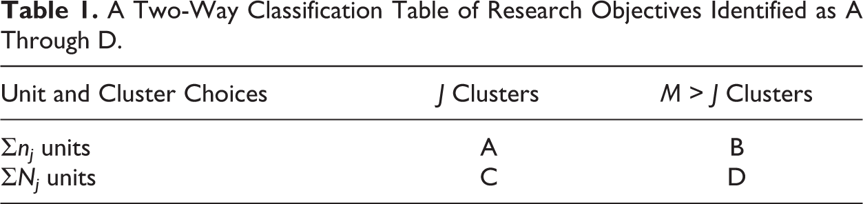
This article assumes that the evaluator seeks to draw statistical inferences about questions that are consistent with cell C. That is, the evaluator seeks to estimate the average treatment effect for the ΣN_j units that could conceptually appear within the fixed J clusters. The author is aware that this is not always the objective. If the J clusters are a probability sample of the M clusters, then the evaluator might make an inference about the M so the focus would be on cell D. The conceptual shift from C to D makes a difference for the estimation problem, and this article will discuss that difference. It is less likely that the evaluator would seek to draw statistical inferences about the Σn_j units rather than the ΣN_j units. Still, cell A is useful for conceptualizing the bias and identification problems posed by CR and PCR designs because important cluster parameters (μ _j or μ _j + δ _j ) are observed⁴ rather than estimated given cell A. Nevertheless, even when cluster parameters are observed, estimates of treatment effectiveness are biased and standard errors are not identified, a point made in this article by presenting the simple variance equation for case A.

The immediate problem considered in this article is (1) why does the bias and identification problem occur and (2) what can an evaluator do to counter the problem? As noted, this problem is discussed elsewhere, but those discussions provide limited insight into the source of the problem, and they may provide ambiguous—and potentially incorrect—advice about estimation. This article provides an intuitive explanation for the problem and, based on that intuition (and some representative mathematics), discusses design and estimation. An expanded companion paper, available from the author, provides mathematical derivations for motivated readers.

Notation

Developing the argument requires Neyman-Rubin’s potential outcome notation. Define Y _ijkt (TR _j ) as the outcome for the ith unit in the jth cluster for the kth pair during period t. The term (TR _j ) indicates that the observations are taken when the cluster is assigned to treatment (TR _j = 1) or when the cluster is assigned to control (TR _j = 0), and only one of these two conditions is observable for a given cluster. Y _ijkt (TR _j ) may be sampled from a larger population within the jth cluster; the cluster population means are μ _jt + TR _j δ _j and variances are $σ_{j t}^{2}$ , where δ _j is the average treatment effect for the jth cluster. When covariates enter the analysis, they are denoted as X _ijkt ; a necessary assumption is that the covariates are independent of treatment assignment, that is, covariates are exogenous. In simple terms, the X _ijkt cannot be determined by treatment assignment.

The notation is redundant because cluster membership determines pair membership; however, at some times the discussion will use index j and at other times it will use index k. The periods are preintervention when t = 1 and postintervention when t = 2. The discussion does not necessarily assume repeated measures (i.e., the same study subjects are observed at preintervention and postintervention), although if repeated measures were available, that availability might be exploited in the estimation, presumably by using change scores or other approaches. There are J clusters, and assuming one-to-one matching, there are K = J/2 pairs. To create the pairs, sort the file based on the average preintervention outcomes using cluster-average measures Y _ijk1 (0) and match so that k = 1 when j = 1 or 2, k = 2 when j = 3 or 4, and so on. (There are other ways to match; Guo & Fraser, 2010; Zhang & Small, 2009; so this approach is illustrative.) Having performed the matching, drop the t subscript because all subsequent calculations will use postintervention data.

At some points in the discussion, the notation is simplified. When using the k subscript without the j subscript, we add a second subscript m, where m = 1 for the first cluster of the kth pair and m = 2 for the second cluster in the pair. This notation will only apply after we have made the matches so we can drop the t subscript and simply write Y _ikm . For simplicity, following randomization within the match pairs, we will always rearrange the order so that m = 1 for the treatment cluster and m = 2 for the control cluster.

Finally, regarding notation, n_j denotes the number of sampled units in the jth cluster, and N_j denotes the population cluster size. Throughout, units comprise a simple random sample from the population, although other probability-based sampling schemes are readily accommodated with suitable notation. The J clusters might be a probability-based sample from a larger population, but assume initially that inferences pertain to treatment effects across the J clusters, not a larger population of clusters, so the sampling of the J cluster is irrelevant. Implications of treating the J clusters as a sample from a larger population are discussed later.

Treating the K Pairs as the Units of Observation

It is possible to think of the data as comprising $\sum n_{j}$ observations, J observations or K observations. All three characterizations are valid, but it will be useful to discuss estimation from the perspective of K observations, each of which provides an estimate of the average treatment effect for clusters within a pair $(δ_{k})$ , namely the mean difference between the outcome for the treatment cluster and the control cluster. The estimated treatment effect across all clusters is then the weighted average of the K pairwise estimates.

\hat{δ} = \sum_{k} ω_{k} {\hat{δ}}_{k} = \sum_{k} ω_{k} (\frac{\sum_{i = 1}^{n_{k 1}} Y_{i k 1}}{n_{k 1}} - \frac{\sum_{i = 1}^{n_{k 2}} Y_{i k 2}}{n_{k 2}}) .

The weights ω sum to one, but beyond that constraint, the evaluator has latitude. The choice of weights is obviously important, given potentially heterogeneous treatment effects. Different estimators discussed in this article and elsewhere apply different weighting schemes and, as a consequence, they may estimate different parameters. Some frequently used estimators estimate parameters that are not easily interpreted.

An evaluator might seek to estimate the average treatment effect when every unit in a population is assigned a weight of one so the average treatment effect for a cluster is given a weight proportional to N_j , and the pair is given a weight proportional to N_k1 + N_k2 . Call this the population average weight. An evaluator might seek to estimate the average treatment effect when every unit in a sample is given a weight of one so the average treatment effect in a cluster is given a weight of n_j , and the pair is given a weight proportional to n_k1 + n_k2 . Call this the sample average weight. The population average weight and the sample average weight are the same, given the sampling is proportional to size. Alternatively, an investigator might seek to estimate the simple average treatment effect across the J clusters. In that case, each cluster receives the same weight as every other cluster. Call this the cluster average weight. Other weights are frequently used including, especially, weighting used to produce efficient estimates of average treatment effects.

Equation 1 implies that an evaluator first estimates the pairwise treatment effect and then averages across the pairs. We prefer this formulation to a regression-based formulation because it is explicit about the weighting and hence about what parameter is being estimated. In contrast, it is often difficult to tell what a regression-based estimator is identifying because the underlying weighting is implicit, a point to which this article turns next.

Regression-Based Estimators

As a contrast to the estimates represented by Equation 1, consider estimators that are based on a regression, such as random effect models and hierarchical models, which use individual-level data. These models implicitly weight the cluster-level treatment effects proportional to the sample size (adjusted for any differences in the unit-level variance within each cluster) plus a constant that appears because of variation in effects across the clusters (i.e. intracluster correlation). Given heterogeneous treatment effects, random effects models and hierarchical models in general do not estimate the same thing as the models discussed in this article. From the perspective of this article, regressions employ a peculiar weighting schemes, driven largely by a quest for efficiency and often (but not necessarily) by an assumption that treatment effects are homogeneous. The estimating equation approach differs because efficiency is seen as a secondary consideration, parameters are typically estimated using the sample size to weight the cluster-level effects, and standard errors are estimated using robust estimation procedures. In summary, regressions based on individual-level data do not necessarily estimate the same parameters as do the cluster-based estimators discussed in this article.

We do not mean this as any implied criticism of using regression models to estimate treatment effects; surely this is an established and venerable approach. Rather, the point is that the cluster-level approach clarifies what is being estimated, a consideration sometimes obscured by regression-based estimates. Another observation is that regression-based approaches appear to be based on a large number of observations: Σn_j . This sample size is misleading, a point emphasized by a sizable literature warning how intracluster correlations inflate standard errors (Cornfield, 1978), but the point is clearer when considering estimation from the cluster-level perspective. A third observation is that regression-based procedures may encourage a thoughtless attitude encouraging use of an apparently more sophisticated but perhaps misleading regression in place of a simpler, readily interpretable cluster-based estimator. Finally, many of the regression-based procedures require some distributional assumptions and those assumptions may be false. Schochet (2012) suggests that evaluators test the sensitivity of their estimates using different estimators, although his approach raises the threat of accepting the estimate that appears best, given the evaluator’s prior opinions. An alternative is to test estimators using baseline data perhaps by using the approaches suggested in the Monte Carlo section on this article. Overall, this article promotes cluster-level estimates on a conceptual level because the cluster-level estimates are transparent about what is being estimated, but it also favors cluster-level estimation on an applied level because of simplicity.

Estimates of Treatment Effectiveness are Biased But Consistent

Starting with the CR design first, a companion paper and the professional literature shows that the CR estimator is biased but consistent as J goes to infinity (Schochet, 2012), provided the size of the treatment effect does not depend on the size of the cluster.⁵ Regardless, the CR estimator will be unbiased if the treatment effects are homogeneous because then the weighting scheme does not matter from a bias perspective.

Moving from Case A to Case C in Table 1, presuming that the sample within each cluster is a simple random sample proportional to size, the story about bias and asymptotic properties does not change. Moving from A to C adds variance to the estimator because the previously known μ _j or μ _j + δ _j must be estimated, but otherwise nothing has changed. Moving from C to D alters the orientation, causing us to think of the data as being a realization of the sample of J clusters from M clusters, and the estimate is unbiased presuming that M is large. (Of course the sampling variance increases when J is treated as a sample from M so just pretending that J is a sample in order to identify the treatment effect is a pyrrhic victory.) We conclude the CR design is biased but consistent in Case C, the case of greatest interest to this article.

Similar storytelling surrounds the PCR design. When J goes to infinity and hence K goes to infinity, the PCR estimator is consistent provided the treatment effect is independent of the sample size (Imai, King, & Nall, 2009) within pairs.⁶ Moving from C to D, the PCR estimate is unbiased provided M is large, but in Case C, the case of greatest interest in this article, the PCR estimator is biased. But PCR is most useful when there are few clusters so asymptotic properties are not compelling, and we must consider bias. Following Imai, King, and Nall—or the proof given in the companion paper—the bias for pairwise matching is given by Equation 2: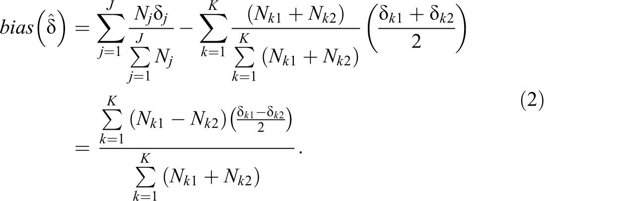

\begin{aligned} b i a s (\hat{δ}) = \sum_{j = 1}^{J} \frac{N_{j} δ_{j}}{\sum_{j = 1}^{J} N_{j}} - \sum_{k = 1}^{K} \frac{(N_{k 1} + N_{k 2})}{\sum_{k = 1}^{K} (N_{k 1} + N_{k 2})} (\frac{δ_{k 1} + δ_{k 2}}{2}) \\ = \frac{\sum_{k = 1}^{K} (N_{k 1} - N_{k 2}) (\frac{δ_{k 1} - δ_{k 2}}{2})}{\sum_{k = 1}^{K} (N_{k 1} + N_{k 2})} . \end{aligned}

In general, the bias represented by Equation 2 will be nonzero, but there are three conditions under which bias disappears, and these conditions have design implications. The first condition is that the intended weighting scheme differs from the one proposed here so that the treatment effect in every cluster receives the same weight, that is, the intention is to estimate a simple cluster-specific average treatment effect. This is seldom the purpose of estimation so this observation provides little comfort. The second condition is that the treatment effect is the same in both clusters of a pair, in which case

δ_{k} = δ_{k 1} = δ_{k 2}

. (The treatment effect can vary across clusters as long as it is constant within pairs.) The third is that the clusters are of equal size so

N_{k 1} = N_{k 2}

within each pair although cluster size can otherwise vary across clusters. Notice that the conditions for unbiased estimation are more lenient in the PCR design than in the CR design because good matching will reduce and potentially eliminate bias.

Unexpectedly, perhaps, random assignment has not guaranteed an unbiased estimate for the treatment effect. Returning to Equation 2, if the problem is that δ and the cluster sizes differ between the clusters within a pair, the bias might still disappear asymptotically, where asymptotic properties depend on the number of pairs increasing to infinity. The intuition is that over a large number of clusters, $(δ_{k 1} + δ_{k 2}) / 2$ will average to $(N_{k 1} δ_{k 1} + N_{k w} δ_{k 2}) / (N_{k 1} + N_{k 2})$ . This asymptotic property will hold, provided the treatment effects are not a function of the cluster size, an assumption that may be reasonable in some settings but not in others. Furthermore, the number of clusters is often a limiting factor so asymptotic properties provide modest comfort. Equation 2 offers some design implications. Before turning to those implication, consider a formula for standard errors of the size of the treatment effect.

Standard Errors Are Not Identified

Using Neyman’s mechanism and applying variance decomposition, a companion paper shows that for cell A in Table 1 the variance for the estimated treatment effects is:

V A R (\hat{δ}) = \sum_{k = 1}^{K} {\{\frac{N_{k 1} + N_{k 2}}{\sum_{k = 1}^{K} N_{k 1} + N_{k 2}}\}}^{2} \{[\frac{σ_{k 1}^{2}}{n_{k 1}} + \frac{σ_{k 2}^{2}}{n_{k 2}}] + {(μ_{k 1} - μ_{k 2})}^{2}\} .

The problem is that while we can estimate the term in brackets, absent making some assumptions, we lack an estimator for the term in parentheses. That is, we can estimate μ _k1 or μ _k2 but not both. (Moving from Case A to C requires the addition of another variance term but does not otherwise resolve the identification problems.) This article will make repeated backward references to Equations 2 and 3 because they are the crux of the problems with bias and identification when dealing with Case C, the case motivating most of the discussion in this article.

Design Considerations

These results are disconcerting. The estimate for the treatment effect is in general biased, and even when it is not, no estimator identifies the sampling variance. These observations have caused some authorities to advise against using the PCR design, but others (Gail et al., 1996) have argued that the biases are typically small, and from a mean-squared error perspective, there is a strong argument for the PCR over the CR design (Imai, King, & Nall, 2009). Nevertheless, making this argument requires some estimator for the variance, considered later when discussing estimators. Prior to that consideration, pause to reflect on some practical aspects of design.

According to Equations 2 and 3, the quality of the match is a key element of estimator performance. According to Equation 2, the bias will be zero when the treatment effects for clusters within a pair are equal: $δ_{k 1} = δ_{k 2}$ . We cannot observe whether this condition holds, but we expect that the condition would hold approximately when the clusters joined in a pair are alike. According to Equation 3, the variance will be identified when, absent treatment, the outcomes for clusters within a pair are equal: $(μ_{k 1} = μ_{k 2})$ . We cannot observe whether this condition holds, but again, we expect that it will hold approximately when the clusters joined in a pair are alike. Good matching is essential.

A second observation follows from the first. A prudent investigator will think carefully about the nature of the treatment effect and, without making assumptions that violate the spirit of random assignment, perform data transformations that will more closely result in additive, homogeneous treatment effects. For example, in the nursing home illustration, it seems sensible to assume that the treatment effect is multiplicative so that the treatment effect varies across units and, specifically, is proportional to the underlying rate of falling for each resident absent the intervention. This suggests estimating the logarithm of the treatment effect for a pair by substituting the logarithm of the mean observed rate of falls for the mean rate of falls in earlier equations. This transformation leads to a model where the logarithm of the treatment effect is plausibly additive and homogeneous within pairs, and consequently, the estimator for the average treatment effect is unbiased. The logarithmic transformation does not guarantee unbiased estimates because the effect can be multiplicative and heterogeneous, but an improved specification is welcome, especially when the transformation only has to work for members of a pair.

A third observation extends the second. In the nursing home illustration, the intervention is partly universal within a nursing home (e.g. removing obstacles that might cause falls for every resident) and partly directed at residents who are predictably at high risk of falling (e.g. case planning for residents based on their fall histories). This suggests that within a nursing home, there are two populations—low-risk and high-risk residents—and that the treatment effect will differ between them. The problem is that the mix of low-risk and high-risk residents may vary across nursing homes, leading to heterogeneity in the treatment effects between nursing homes within a pair. However, if high- and low-risk populations can be distinguished using statistical procedures, the bias might be reduced or removed by poststratification and estimation of the two treatment effects, one for low-risk residents and one for high-risk residents. Because randomization was not predicated on risk, poststratification is a valid estimation strategy.⁷ Continuing to extend this reasoning, the bias might be further reduced by introducing covariates into the analysis instead of or in addition to using poststratification, but discussion of that special topic is reserved because introducing covariates requires special (but simple) manipulation of the data.

Putting these observations together, they imply strategies for reducing bias in the estimated treatment effect and identifying the standard error. With regard to the standard error, looking at Equation 3, a close match will drive the term in parentheses toward zero, and using prestratification to adjust for cluster characteristics and poststratification to adjust for unit characteristics may additionally improve the nearness of the match. The variance is identified or nearly identified. With regard to bias, looking at Equation 2, matching is important to assure that cluster members of each pairs have the same average treatment effects, and beyond pairing, homogeneity of the treatment effect within pairs can be promoted by data transformations, prestratification based on cluster characteristics, and poststratification based on unit characteristics. None of this is doable without substantive knowledge of the programs being evaluated so evaluation is not the exclusive province of statisticians; still, good evaluation requires basic understanding of design considerations.

The discussion assumed matching on preintervention outcome measures, and while this is an attractive strategy for matching, other strategies must be employed when preintervention outcome measures are unavailable (Hayes & Moulton, 2009, p. 77). The absence of good matching variables is one of the reasons why the Medical Research Council (2002) cautioned against using pairwise matching. Furthermore, the use of an alternative matching strategy is required when there are multiple outcome measures.⁸ The relative preference for PCR and CR, and of an intermediate position of stratification into blocks (Hayes & Moulton, 2009; Imbens, 2011),⁹ is likely to differ across disciplines and evaluation topics. In an age of information technology, preintervention outcome measures are often accessible through information systems, increasing the quality of the matches, and the justification for using PCR. However, if an investigator’s concern is with public health interventions in a developing nation, for example, preintervention outcomes measures may be unavailable, and stratification based on location or other observable criteria may be best. The pairwise match might be seen as good in the former case, leading to the PCR design, and questionable in the latter case, leading to a CR design.

Regardless of how he or she matches, an investigator must be mindful of why he or she is matching and that is the principal subject of this section. Most discussions of this topic concern variance reduction, a topic to which this article turns in the following sections, but from Equations 2 and 3, we see that variance reduction is not the only important consideration when matching. From Equation 2, we see that estimation will be least biased if matched clusters have about the same population sizes, and if the size of the treatment effect is about the same within pairs or at least not widely different. From Equation 3, we see that the estimate of the variance will be identified if the mean outcomes in the counterfactual state are the same in the postintervention period. These observations require that the matching criteria be prospective; perhaps the past is prologue but this need not be true. We are using the past to anticipate the future, but a mechanical application of past commonalities among clusters should not substitute for a consideration of future commonalities among clusters including anticipation of capacity and willingness of clusters to implement treatment. The nursing home evaluation is using a mixed strategy of pair matching (based on retrospective data) and stratification (based on the anticipated willingness and ability of homes to implement the intervention). These are forward-looking criteria, which presume that the past is indicative of the future but that anticipate, based partly on subjective assessment, the ability and willingness of nursing homes to successfully implement the treatment.

In sum, knowledge of the substantive problem and thoughtful design can overcome or at least minimize the bias in the estimated treatment effect, a useful observation from a mean-squared error perspective, given that the PCR design can be much more efficient than the CR design. This article has not presented an estimator for the variance, but the following two sections on nonparametric and parametric estimation discuss that issue, after which the article turns to the question of whether and when the PCR design is more efficient than the CR design.

Traditional Nonparametric Solutions

There are two generic forms of estimators for δ, one nonparametric and the second parametric or semiparametric. This section considers the nonparametric estimator. The discussion is introductory and elementary; readers who seek to go beyond this rudimentary summary might consult Sprent and Smeeton (2007). Throughout this section, assume one-on-one matching, and assume that the clusters are about the same size or, if the clusters are not about the same size, that the error distributions are not grossly asymmetric. These are innocuous assumptions (Murray, 1998, p. 116), and interested readers can learn about consequences in rare cases where they fail (Gail et al., 1996).

The Wilcoxin sign rank test makes no distributional assumptions other than an innocuous assumption regarding symmetry. The associated Hodges–Lehman estimator leads to point estimates and confidence intervals. The sign rank test (1) starts with the absolute values of the K estimated treatment effects, (2) ranks then from high to low, assigning 1 to the low rank and K to the high rank, and (3) then sums the ranks for when the k estimated treatment effects are positive. The sum of the ranks is the test statistic. Under the null, the sum of the ranks for the negative and positive outcomes should be about equal, so in expectation the sum S will equal $\sum_{k = 1}^{K} k / 2 = K (K + 1) / 4$ . There is a small probability (1/2) ^K that the sum could be as large as $\sum_{k = 1}^{K} k$ , that is, that the rank score is positive for all K pairs, a somewhat smaller probability that it is positive for K − 1 of the pairs, and eventually a probability of .05 or less it is positive for K, K − 1 … K − C pairs. For a one-tailed test, K − C identifies the critical value of the test statistic.

The Hodges–Lehmann estimator lacks the intuitive appeal of the sign rank test itself, and we will not provide an explanation for deriving a point estimate and confidence intervals. Interested readers might consult Sprent and Smeeton (2007, p. 53) for one explanation and Rosenbaum (2009, p. 43) for an explanation from an alternative perspective. The important point is that we can derive a nonparametric test statistics for the null of no treatment effect, a point estimate for the median treatment effect, and confidence intervals for the median treatment effect without making distributional assumptions—a good thing, given that the variance discussed earlier is not identified.

However, the Hodges–Lehmann estimator leads to an estimated median across the clusters using what was previously called a cluster average weight. Because of symmetry the median should be close to the mean based on the population or sample average weights, provided the clusters are about the same size. If the clusters have much different sizes, however, the Hodges–Lehmann estimator may be much different from the parametric estimators.

The nonparametric estimator has desirable features and is more consistent with the spirit of random assignment than are parametric estimators. The estimated treatment effect is no longer biased, although this quality is purchased at the price of using cluster average weights to identify the median effect across the clusters. There is no need to estimate a sampling variance (i.e., Equation 3) because the permutation test depends exclusively on the design. There is a large sample variance approximation, but this too comes from the design, not the data and specifically does not depend on knowing μ _k1 − μ _k2 . In the spirit of random assignment, the nonparametric estimator has much to recommend it, although its utility is limited when K is small, and it does come at the cost of reduced efficiency compared with the parametric estimator, discussed next.

Parametric, Partially Parametric, and Other Nonparametric Solutions

Nonparametric tests are in the spirit of random assignment because no distributional assumptions are required to interpret test statistics or to derive point estimates and confidence intervals. But by making distributional assumptions, the same sort of assumptions seen as largely innocuous in other settings, we can increase power. So what should be said about substituting parametric estimators for nonparametric estimators? Whatever can be said in general about the substitution, the PCR design poses special problems that stem from random sampling within pairs. The nature of the problem has already been discussed: With the data at hand, we cannot estimate the variance represented in Equation 3 without making additional assumptions. To illustrate the difficulty, and to introduce a regression-based estimator, consider a fixed-effect regression estimator (Bloom, 2005).

Bloom’s (2005) specification is a simple linear model where K dummy variable represents the matched clusters and an additional dummy variable represents the receipt of treatment. The companion paper shows that this estimator reduces to the estimator shown by Equation 2 except for the weighting scheme. In Equation 2, the weights were proportional to N _k ₁ + N _k ₂, so the bias was with respect to the population average weights. Now the weights are proportional to n_k1 + n_k2 . Substituting this new weighting scheme into Equation 2 leads to the conclusion that the estimated treatment effect is biased. The earlier discussion of using design for reducing bias continues to apply, and, moreover, there is really no need for this distinct regression-based estimator. Estimation based on cluster-level summaries will work just as well and they will not obscure the weighting scheme.

The estimated variance is again problematic. Based on results shown in the companion paper, Equation 3 still represents the problem, provided we substitute the sample-specific weights for the population-specific weights. As before, the problem is that we cannot estimate the term in parentheses Δ = μ _k1 − μ _k2 .

In practice, an evaluator would likely not estimate the regression with the above-mentioned specification. He or she might instead apply a more efficient generalized least squares estimator. The Monte Carlo simulation in fact adjusts the fixed-effect estimator to account for heteroscedasticity, although this adjustment is only partial because it does not adjust for the unknown Δ. Adjusting for heteroscedasticity is likely to improve efficiency but, as already shown, does not eliminate the problem with bias. Furthermore, when the treatment effect is heterogeneous across clusters, we cannot be sure that the regression is actually estimating.

We have purposefully shown the regression estimator can be expressed as a cluster-level estimator that adopts a specific weighting scheme, thereby demonstrating that in general the fixed-effect least square estimator will lead to a biased standard error for the estimated treatment effect. Imai, King, and Nall (2009, p. 36) suggest a nonparametric variance estimator that provides an upper limit on the variance regardless of the weighting scheme. Using the notation from this present article, their estimator is:

\begin{array}{l} V A R {(\hat{δ})}_{P C R, I K N} = \\ \frac{K}{(K - 1)} {\sum_{k = 1}^{K} [w_{k} {T R_{k} (\frac{\sum_{i = 1}^{n_{k 1}} Y_{i k 1}}{n_{k 1}} - \frac{\sum_{i = 1}^{n_{k 2}} Y_{i k 2}}{n_{k 2}}) + (1 - T R_{k}) (\frac{\sum_{i = 1}^{n_{k 2}} Y_{i k 2}}{n_{k 2}} - \frac{\sum_{i = 1}^{n_{k 1}} Y_{i k 1}}{n_{k 1}})} - \frac{1}{K} \hat{δ}]}^{2}, \end{array}

where w_k is one of several weighting schemes that sum to 1 and

\hat{δ}

is the estimated average treatment effect across the paired clusters, written as:

\begin{aligned} \hat{δ} = \sum_{k = 1}^{K} w_{k} {\hat{δ}}_{k} \\ = \sum_{k = 1}^{K} w_{k} \{T R_{k} (\frac{\sum_{i = 1}^{n_{k 1}} Y_{i k 1}}{n_{k 1}} - \frac{\sum_{i = 1}^{n_{k 2}} Y_{i k 2}}{n_{k 2}}) + (1 - T R_{k}) (\frac{\sum_{i = 1}^{n_{k 2}} Y_{i k 2}}{n_{k 2}} - \frac{\sum_{i = 1}^{n_{k 1}} Y_{i k 1}}{n_{k 1}})\} . \end{aligned}

Both the treatment effect and the upper limit for its sampling variance are easily estimated by combining cluster-level estimates. The sample statistic is treated as being distributed as Student’s t with K − 1 degrees of freedom. Improvements are possible; interested readers should consult Imai, King and Nall.

It is disconcerting that we cannot estimate the sampling variance, although estimating an upper limit, and designing the analysis to cause the upper limit to be near the true variance, is comforting. There is another way to proceed, which rests on some assumptions and the availability of preintervention data. The necessary assumption is that Δ _k = μ _k1 − μ _k2 does not change from the preintervention period to the postintervention period. This is equivalent to assuming that the mean outcomes under the counterfactual states do not change from the preintervention period to the postintervention period, or if they change, the change is the same for each cluster in every pair of clusters. Then we can estimate Δ_k using preintervention data, and from Equation 3 we can estimate the sampling variance. (An alternative is to assume that Δ _k is the same for all k.) This is admittedly an ad hoc justification.¹⁰

Some generalizations follow from these results. Equation 3 shows that we can reduce variance, to a point, by leaving K fixed and increasing n, but we cannot force the variance to zero without increasing the number of pairs. Apparently, we can reduce the variance toward zero by increasing the number of pairs toward infinity (Schochet, 2012), although this sanguine implication is misleading. The availability of clusters is typically fixed, relatively small, and where large, may be inaccessible because of budget constraints.

This subsection has illustrated a fundamental problem with the PCR design, namely, lack of a straightforward method for estimating Δ _k . Here, the Wilcoxin sign rank test and the Hodges–Lehmann estimator have advantages, partly offset or course by the fact that the nonparametric estimator is less efficient than its parametric counterpart and that the nonparametric approach estimates the median across the clusters, but in the spirit of random assignment—where avoiding assumptions is desirable—the nonparametric estimator has a clear advantage. Perhaps we should not worry too much about the problem and concentrate on making good matches so that the unknown variance component becomes negligible.

Readers of other articles regarding PRC will note the absence of the term intercluster correlation coefficient, often expressed as ρ_A and written as $ρ_{A} = Δ^{2} / (σ^{2} + Δ^{2})$ . Most treatments of PCR begin with ρ_A so where has it gone? Assuming that Δ is the same across clusters, applying the sample weights, solving for Δ², the companion paper shows that the variance term can be expressed using the intercluster correlation coefficient:

V A R (\hat{δ}) = [\frac{2}{n} + \frac{ρ_{A}}{1 - ρ_{A}}] \frac{σ^{2}}{K} .

The rhetoric is that we cannot estimate the variance because we cannot estimate ρ_A but obviously this is the same as not being able to estimate Δ. Nevertheless, this observation ties the discussion in this article into discussions presented in standard sources. Although comparable derivations appear elsewhere, the current derivation—which uses the Neyman mechanism to treat the variance as arising from a sampling problem—clarifies the source and importance of the intercluster correlation coefficient.

PCR or Cluster CR?

Is PCR always better than a simpler CR design? To answer that question, consider an intuitive argument before turning to a more formal argument. Across the population of clusters, the investigator can observe J mean outcomes. Using a CR design, after random assignment an investigator will be able to estimate μ _j + δ _j for 1 … K of these clusters and μ _j for K + 1 … J of these clusters. By chance the investigator might have randomly sampled for treatment K clusters that had the lowest values of μ _j + δ _j , in which case the estimated treatment effect would be much too low; alternatively, by chance the investigator might have randomly sampled for treatment K cluster that had the highest values of μ _j + δ _j , in which case the estimated treatment effect would be much too high. Given random assignment, the extreme highs and lows will balance, but the sampling variance will be high. The relative advantage of the PCR design is that good matching will reduce the probability that these extreme outcomes will occur so that on this ground, the PCR estimator is more efficient than the CR estimator. Somewhat offsetting this advantage is that the CR design provides J data points and J − 2 degrees of freedom for the test statistic based on an unmatched t-test, while the PCR design provides K data points and K − 1 degrees of freedom based on a matched t-test. This reduction in degrees of freedom affects the test statistic and the confidence interval (Klar & Donner, 1997; Martin, Diehr, Perrin, & Koepsell, 1993) because the shape of the t-distribution depends on the degrees of freedom. For example, to reject the null hypothesis using a one-tailed test requires a test statistics of 2.02 when the degrees of freedom equal 5, a test statistics of 1.82 when the degrees of freedom equal 10, a test statistics of 1.75 when the degrees of freedom is 15, and the familiar a test statistics of 1.65 when the degrees of freedom is large.

This degree of freedom disparity has led to an often repeated rule of thumb that the PCR design should be considered only when there are 10 or more pairs (Diehr, Martin, Koepsell, & Cheadle, 1995; Feng, Diehr, Peterson, & McLerran, 2001), although this rule of thumb is qualified by its proposers, and it is disputed by others (Imai, King, & Nall, 2009). This article recommends avoiding the rule of thumb in favor of an approach explained in the Monte Carlo section of this article.

The companion paper shows that the efficiency of the PCR design depends on two factors. The first is the proportion of variance contributed by intracluster correlations. If it is negligible—that is, if there is little variation in μ_j across the clusters—then neither design is superior in terms of efficiency. (We would be concerned with lost degrees of freedom from the PCR design, so the CR design would be preferred.) Intuitively, the evaluator had no chance to make “bad draws” when assigning clusters to treatment and control. Otherwise, for the PCR design to be more efficient, the companion paper shows that the following inequality must hold:

\frac{\sum_{k = 1}^{K} {(μ_{k 1} - μ_{k 2})}^{2}}{J^{2}} < \frac{\sum_{j = 1}^{J} {(μ_{j} - \overset{ˉ}{μ})}^{2}}{J^{2}} .

The inequality is not especially intuitive although it does emphasize that while the evaluator has no control over the term of the right of the inequality (i.e., the CR design), matching provides some control over the term on the left (i.e., the PCR design). The Monte Carlo experiment will illustrate one method for judging whether the inequality holds and, with due consideration for the degrees of freedom, whether the PCR design provides a narrower confidence interval for the average treatment effect than does the CR design.

The comparison is not altogether fair or, at least, not altogether complete. So far the approach has not employed covariates—the X _ijk variables identified earlier. Introducing covariates can greatly alter the problem, perhaps even reversing decisions made on Equation 7 alone. The introduction of covariates is the next topic.

Introducing Covariates

Although there are nJ study subjects, insight has come from reducing the data points to K for the PCR design. Evaluators may be uncomfortable with this reduction; where has all the data gone? What can we do with covariates measured at the unit level; what can we do with cluster-level covariates? There are many ways to introduce covariates into the estimation, depending on the evaluator’s tolerance for assumptions. Hayes and Moulton (2009, p. 237) recommend a two-step approach that is applicable to nonparametric estimators (Gail et al., 1996, p. 1086; Rosenbaum, 2009) and parametric estimators. Readers were notified earlier that this article will not discuss comparatively familiar one-step procedures, which are discussed in textbooks about cluster randomization (Donner & Klar, 2000; Hayes & Moulton, 2009; Murray, 1998) and specialty texts (Baltagi 2005; Bryk & Raudenbush, 1992; Cameron & Trivedi, 2005; Gelman & Hill, 2007).

The first step uses a regression to estimate the conditional mean of the outcome, omitting a treatment variable from the specification. To understand this approach, study Equation 8, the assumed data generation process (DGP) after the intervention:

Y_{i k m} (T R_{k m}) = ξ_{k m} + X_{i k m} β + T R_{k m} δ_{k m} + e_{i k m} .

This assumed DGP has a fixed-effect specific to each cluster, and it allows, but does not require, the treatment effect to vary across clusters. Now, instead of using a dummy variable for every cluster, use a dummy variable for every pair, leading to a revised model specification with a modified error term shown in parentheses:

Y_{i k m} (T R_{k m}) = α_{k} + X_{i k m} β + T_{k m} δ_{k m} + (e_{i k m} + ξ_{k m} - α_{k}) .

Next, drop the treatment variable and incorporate the omitted treatment variable into the error term:

\begin{aligned} Y_{i k m} (T R_{k m}) = α_{k} + X_{i k m} β + (T R_{k m} δ_{k m} + e_{i k m} + ξ_{k m} - α_{k}) \\ = α_{k} + X_{i k m} β + u_{i k m} . \end{aligned}

The first step in the two-step approach is to estimate a regression consistent with this DGP and to use the parameter estimates from that regression to estimate the error terms u_ikm, which is estimated consistently from a regression based on Equation 10 because the error term is independent of the fixed pair effects and the covariates. Consistency requires that the sample size goes to infinity in each pair (McCulloch & Searle, 2001).

The second step is to substitute the residuals from Equation 10 for the Y _ikm (TR _km ) in earlier equations. The matching would be performed based on the average size of the residuals for each cluster. There are three expected consequences: (1) the bias in the estimated treatment effect will be reduced; (2) the standard error for the estimated treatment effect will be reduced; and (3) the estimates of the standard errors will be improved in the sense that the addition of covariates has reduced the problem with identification.

Although we have introduced covariates into the analysis, the conceptualization of the problem and its solution remains at the cluster level. We have simply readjusted the cluster means to partial out (or control for) the effect of factors that differentiate units. This can lead to better matches and to statistics with better properties for statistical inference. The cost is that the evaluator must depart from the pure random design tradition and specify a statistical model, but the model is testable so this departure seems innocuous and can improve estimates of the treatment effect.

Monte Carlo Illustrations

Monte Carlo simulations are often used to investigate the properties of estimators. Sometimes the simulation examines extreme conditions to discover how well an estimator performs under those extreme, sometimes unrealistic conditions. The simulations reported in this article have a different flavor. An investigator is faced with a problem: Should he or she use a CR design instead of a PCR design? If a PCR design, should he or she use a parametric or nonparametric estimator? And if the former, which of the variance estimators discussed earlier is preferable? Is power adequate to justify the study? With baseline data and some assumptions, an investigator can approximate the properties of the estimators and make a reasoned decision about design and analysis. This article uses Monte Carlo simulation in the context of recommending a design step that investigators could take in practice.

Again using the nursing home evaluation to illustrate, the simulation starts with the known preintervention rate of falls¹¹ in every nursing home and assumes that falls are generated by a Poisson process so that the rates and variances are the same within a nursing home. It treats the rate and variance as population parameters determined by the observed preintervention data. The simulation requires three steps repeated over 100,000 replications: In the first step, given the population parameters, it samples a new rate parameter to serve as the preintervention rate.¹² Based on that preintervention rate parameter, it matches the J = 26 nursing homes to create K = 13 pairs, and it randomly assigns one member of every pair to the treatment condition. In the second step, the simulation resamples a new rate parameter and adds a treatment effect equal to δ times that rate parameter; these serve as the postintervention data. In the third step, the simulation applies various estimators to the simulated postintervention data. The simulation is repeated 100,000 times and accumulates (1) the average estimated treatment effect across the 100,000 replications, (2) the standard deviation for the estimated average treatment effect across the 100,000 replications, and (3) the average estimated standard errors for each of the estimated treatment effects across the 100,000 replications.

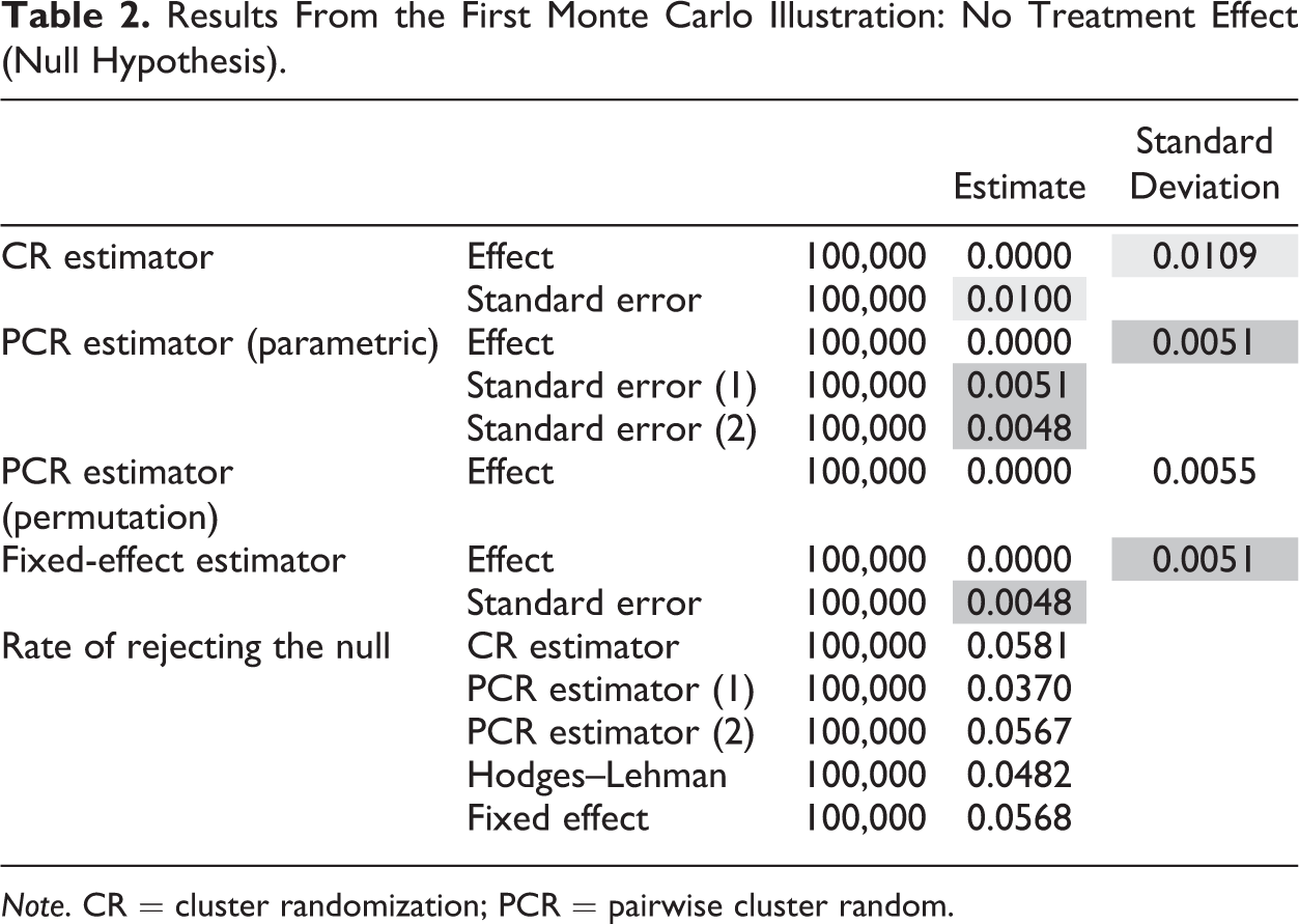
The simulation uses four estimators for each replication: the CR estimator, the parametric PCR cluster-level estimator, the nonparametric (permutation) cluster-level estimator, and the fixed-effect regression estimator. The parametric PCR estimator has two variance estimators: the first is the estimator that uses the preintervention data to estimate Δ and the second is the upper limit estimator. The tables report the observed standard deviation (based on the 100,000 replications) across the estimates in the last column and the average of the estimated standard errors across the estimates in the previous column. Shading links the standard deviations with the corresponding average of the estimated standard errors.

Results are reported in Table 2 when the null hypothesis of no treatment effect (δ = 0) is true. The first estimator is the CR estimator. The CR estimator requires some estimate of the intracluster correlation, and it uses a moment-based estimator from Stata’s metan procedure. The second estimator is the PCR estimator based on the parametric model. The third is the estimator based on the nonparametric model; the simulation uses Stata’s cendif program, which provides confidence intervals for Hodges–Lehmann median differences (Newson, 2002). The fixed-effect estimator is based on a weighted least square regression with fixed effects for the pairs; the simulation uses Stata’s reg procedure with aweights, which are the inverse of the estimated square standard errors for the cluster estimates ignoring the intercluster correlation. The statistic reported in the lower part of the table is the proportion of time across 100,000 replications that the estimated confidence intervals fail to overlap 0. These should be close to 0.05 under the null of no treatment effect.

Table 2.

Results From the First Monte Carlo Illustration: No Treatment Effect (Null Hypothesis).

			Estimate	Standard Deviation
CR estimator	Effect	100,000	0.0000	0.0109
	Standard error	100,000	0.0100
PCR estimator (parametric)	Effect	100,000	0.0000	0.0051
	Standard error (1)	100,000	0.0051
	Standard error (2)	100,000	0.0048
PCR estimator (permutation)	Effect	100,000	0.0000	0.0055
Fixed-effect estimator	Effect	100,000	0.0000	0.0051
	Standard error	100,000	0.0048
Rate of rejecting the null	CR estimator	100,000	0.0581
	PCR estimator (1)	100,000	0.0370
	PCR estimator (2)	100,000	0.0567
	Hodges–Lehman	100,000	0.0482
	Fixed effect	100,000	0.0568

Note. CR = cluster randomization; PCR = pairwise cluster random.

Under the null, the estimated treatment effects should be near 0 over 100,000 replications and that is true for all four estimators. The most noteworthy comparison afforded by this table is between the standard deviation for the CR estimator and the standard deviation for any of the PCR estimators. (See the last column.) The improvement is greatest for the parametric estimators, and it is lesser for the nonparametric estimator. There is little justification for using the CR estimator. Although the simulation suggests that the PCR estimator is more efficient than the CR estimator, little is lost by using the nonparametric estimator instead of one of the parametric estimators, and given that the Monte Carlo simulation has had to make some distributional assumption (Poisson) that might be wrong, there is a strong argument for the nonparametric estimator.

The shading is intended to assist when comparing the true standard deviation across the simulations with the average of the estimated standard errors across the simulations. Comparing the standard deviations with the average for the estimated standard errors, the variance estimates all appear to perform reasonably well, although all understate the variance somewhat. It seems strange that the upper limit estimator is actually less than the standard deviation.

Ideally, the estimators should reject the null with probability .05. The Hodges–Lehman estimator cannot achieve that goal because of a limitation to the permutation test; however, the achieved limit is 0.046143 and that is consistent with this simulation. Looking at the parametric estimators, while the coverage is not precise, the bias when estimating the standard error does not appear serious.

Table 3 has the same structure as Table 2. For Table 3, the simulation assumes a multiplicative treatment effect equal to 0.25, meaning that the rate of falls is reduced by 0.25 in the treatment nursing homes. Because the simulation estimates the treatment effect as being additive, however, the average additive treatment effect built into the simulation is −0.0201.¹³ The purpose of this “misspecification” is to demonstrate the effect of heterogeneous treatment effects. The median is −.01963.

Table 3.

Results From the Second Monte Carlo Simulation: Treatment Effect of −0.0201 (Mean) and −0.01963 (Median).

			Estimate	Standard Deviation
CR estimator	Effect	100,000	−0.0201	0.0096
	Standard error	100,000	0.0095
PCR estimator (parametric)	Effect	100,000	−0.0202	0.0045
	Standard error (1)	100,000	0.0048
	Standard error (2)	100,000	0.0045
PCR estimator (permutation)	Effect	100,000	−0.0191	0.0049
Fixed-effect estimator	Effect	100,000	−0.0183	0.0046
	Standard error	100,000	0.0045
Rate of rejecting the null	CR estimator	100,000	0.6776
	PCR estimator (1)	100,000	0.9955
	PCR estimator (2)	100,000	0.9951
	Hodges–Lehman	100,000	0.9710
	Fixed effect	100,000	0.9797

Note. CR = cluster randomization; PCR = pairwise cluster random.

All the estimators do a tolerable job of recovering the average treatment effect of −0.0201. The nonparametric estimator appears to be less accurate than the parametric estimator, but in fact the nonparametric estimator is recovering the median, explaining the discrepancy. (The treatment effect averaged between the 13th and 14th nursing home is −0.0196.) The fixed-effect estimator appears to understate the treatment effect, and this illustrates an earlier observation about the fixed-effect estimator. The weighted least squares version of the fixed-effect estimator attempts to recover an efficient estimate under an assumption that the effects are homogeneous, and consequently, the fixed-effect estimator employs a different weighting scheme than do the other estimators. Instead of weighting by N_k1 + N_k2 , it attempts to weight by the inverse of $\frac{σ_{k 1}^{2}}{n_{k 1}} + \frac{σ_{k 2}^{2}}{n_{k 2}}$ . Given a Poisson assumption, the nursing homes with the lowest rate of falls will have larger weights than the nursing homes with the highest rate of falls, and the former will have smaller treatment effects than the latter, explaining why the fixed-effect estimator is biased downward.

Perhaps the most telling statistic is the power. As expected, the CR design has the least power, rejecting the null in 67.8% of the repetitions. This is followed by the nonparametric PCR design and the parametric PCR designs, respectively. Using PCR, the study is highly powered to detect a treatment effect that reduces falls by about 25%.

The next simulation sets the multiplicative treatment effect to 0.10. Given the additive units used in the simulation, the average treatment effect is −0.0081 and the median is −0.0079. Table 4 shows the results.

Table 4.

Results From the Third Monte Carlo Simulation: Treatment Effect of −0.0081 (Mean) and −0.0079 (Median).

			Estimate	Standard Ddeviation
CR estimator	Effect	100,000	−0.0080	0.0104
	Standard error	100,000	0.0096
PCR estimator (parametric)	Effect	100,000	−0.0081	0.0048
	Standard error (1)	100,000	0.0050
	Standard error (2)	100,000	0.0046
PCR estimator (permutation)	Effect	100,000	−0.0076	0.0052
Fixed-effect estimator	Effect	100,000	−0.0073	0.0049
	Standard error	100,000	0.0046
Rate of rejecting the null	CR estimator	100,000	0.2039
	PCR estimator (1)	100,000	0.4335
	PCR estimator (2)	100,000	0.4901
	Hodges–Lehman	100,000	0.3843
	Fixed effect	100,000	0.4319

Note. CR = cluster randomization; PCR = pairwise cluster random.

Table 4 demonstrates nothing that was not demonstrable in Table 3, except that Table 4 shows how the Monte Carlo simulation might be used to estimate power. The power for the CR estimator is clearly unacceptable for identifying a treatment effect as low as a 10% reduction in falls. The power for the other estimators do not reach conventional standards of 0.8 so likely we would conclude that no study design could reliably detect a treatment effect as small as the one built into this final simulation.

In some regards, the simulation is too optimistic. It assumes that falls are distributed according to a Poisson process, but it seems more realistic to assume an overdispersed Poisson process. A dispersion parameter could be built into the simulation, but without individual-level preintervention data, it is difficult to anticipate a realistic dispersion parameter. In other regards, the simulation is too pessimistic because it does not assume any adjustments for covariates that will actually be available at the time of data analysis.

There is one other way that the simulation is too pessimistic. In the Monte Carlo simulation, the preintervention and postintervention samples are treated as random draws from known population distributions. In the nursing home illustration, it seems likely that some nursing home residents who were in the nursing home during the preintervention period will remain in the nursing home during the postintervention period. If so, there will be a closer correlation between the preintervention and postintervention data, and consequently, the pairing will be better than is assumed in this simulation and power will be understated.

A Monte Carlo simulation cannot demonstrate that one estimator is better than the other in general, and such a demonstration was not the point of this exercise. Rather, this exercise provided concrete steps for discovering how an estimator is likely to behave based on what is known about preintervention outcomes and what is assumed about the data generation process. Especially useful is the demonstration that while the parametric estimators are biased and while their standard errors are approximate, the bias is small and the approximations are reasonably precise. We could not know this from theory alone. The exercise can also be used to estimate power. In short, the exercise is worthwhile for making design decisions.

Observations

To this point the argument has been descriptive; now the argument shifts to advocacy. As the argument developed, it assumed availability of baseline data used to form the matches. What if the baseline data do not exist? Many evaluators have matched clusters based on cluster characteristics, but this may lead to poor matches if there is no strong logic model linking those characteristics with prospective outcomes, leading to the concern that estimates of treatment effectiveness based on K observations may be less efficient than estimates of treatment effectiveness based on J observations. Score one point for advocates of the CR design.

Whatever the historical record shows about the availability of baseline data, modern evaluators live in an era during which baseline data are frequently available as administrative records. For example, in the nursing home illustration, the nursing homes were able to report the rate of falls for every nursing home during the year before matching occurred. In fact, the nursing home evaluation team is in the process of acquiring the baseline data for every resident across those nursing homes, providing the means to introduce covariates into the design and estimation. Baseline data are increasingly available across health care and social intervention settings, leading to the belief that use of the PCR design is—or should be—on the ascendency.

There remain some technical concerns with identification when using the PCR design. Although perceptions of technical concerns have sometimes inhibited investigators from using the PCR design or caused them to take very conservative steps when designing studies to yield acceptable power, consistent with the arguments made by others, this article argues that the PCR design has advantages in terms of mean-squared error. Furthermore, in an era of easily accessible administrative data, use of a PCR design does not have to rest on a hope and a prayer ensured by unnecessarily large and consequently expensive sample sizes. An investigator can perform useful design tests of estimator performance and power. Conservatism may be warranted but ultraconservatism is wasteful. Finally, many evaluators—especially those in education settings—have the luxury of working with large numbers of clusters, in which case asymptotic properties are likely to yield precise approximations so bias and identification are not so important.

This article has advocated cluster-level analysis in contrast to individual-level analysis, where the latter often takes the form of random effects models in econometrics and hierarchical models across other disciplines. Models suitable for individual-level analysis surely have their places in behavioral research but individual-level analysis tends to obscure what the evaluator must consider when performing a good cluster random design experiment. For example, many of us have trouble unscrambling the weighting used in a hierarchical model and therefore have difficulty understanding what the hierarchical model is actually estimating. Unfairly, perhaps, we are concerned that investigators sometimes “throw a regression at a problem” with the hope or even expectation that the sophisticated regression will reveal something that otherwise will remain obscure using simpler estimators.

This article has taken a different perspective. Starting with cluster-level analysis, and using Neyman’ mechanism, this article has provided an intuitive explanation for why intercluster and intracluster correlations matter when estimating treatment effects. This article has demonstrated that the cluster-level approach is a good way to analyze data, keeping the investigator closer to the random design tradition and preventing the sophistication of an estimator from obscuring what that estimator is actually estimating.

Footnotes

Declaration of Conflicting Interests

The author(s) declared no potential conflicts of interest with respect to the research, authorship, and/or publication of this article.

Funding

The author(s) received no financial support for the research, authorship, and/or publication of this article.

Notes

References

Baltagi

(2005). Econometric Analysis of Panel Data (3rd ed.). New York, NY: John Wiley.

Becker

Krin

Lindermann

Sturm

Eichner

Walter-Young

Nikolaus

(2003). Effectiveness of a multifaceted intervention on falls in nursing home residents. Journal of the American Geriatrics Society, 51, 306–313.

Berk

(2005). Randomized experiments as the bronze standard. Journal of Experimental Criminology, 1, 417–433.

Bloom

(2005). Randomizing groups to evaluate place-based programs. In Bloom

(Ed.), Learning more from social experiments: Evolving analytical approaches (pp. 115–172). New York, NY: The Russell Sage Foundation.

Bryk

Raudenbush

(1992). Hierarchical linear models. Newbury Park, CA: Sage.

Cameron

Trivedi

(2005). Microeconometrics: Methods and applications. Cambridge, UK: Cambridge University Press.

Cheung

Jeffries

Thomson

Milligan

(2008). A simple approach to test for interaction between intervention and an individual-level variable in community randomization designs. Tropical Medicine and International Health, 13, 247–255.

Cornfield

(1978). Randomization by group: A formal analysis. American Journal of Epidemiology, 108, 100–102.

Diehr

Martin

Koepsell

Cheadle

(1995). Breaking the matches in a paired T-test for community interventions when the number of pairs in small. Statistics in Medicine, 14, 1491–1504.

10.

Donner

Klar

(2000). Design and analysis of cluster randomization trials in health research. West Sussex, UK: John Wiley.

11.

Donner

Klar

(2004). Pitfalls and controversies in cluster randomization trials. American Journal of Public Health, 93, 416–422.

12.

Feng

Diehr

Peterson

McLerran

(2001). Selected statistical issues in group randomization trials. Annual Review of Public Health, 22, 167–187.

13.

Gail

Mark

Carroll

Green

Pee

(1996). On design considerations and randomized-based inference for community intervention trials. Statistics in Medicine, 15, 1069–1092.

14.

Gelman

Hill

(2007). Data analysis: Using regression and multilevel/hierarchical models. Cambridge, UK: Cambridge University Press.

15.

Guo

Fraser

(2010). Propensity score analysis: Statistical methods and applications. Thousand Oaks, CA: Sage.

16.

Hayes

Moulton

(2009). Cluster randomization designs. London, UK: Chapman & Hall/CRC Interdisciplinary Series.

17.

Heckman

Vytlacil

(2007a). Econometric evaluation of social programs, Part I: Causal models, structural models and econometric policy evaluations. In Heckman

Leamer

(Eds.), Handbook of Econometrics Volumne 6B (pp. 4780–4874). Amsterdam, the Netherlands: North Holland Press.

18.

Heckman

Vytlacil

(2007b). Econometric evaluations of social programs, part II: Using the marginal treatment effect to evaluate social programs, and to forecast their effects in new environments. In Heckman

Leamer

(Eds.), Handbook of Econometrics Volume 6B (pp. 4878–5143). Amsterdam, the Netherlands: North-Holland Press.

19.

Hill

Scott

(2009). Comment: The essential role of pair matching. Statistical Science, 24, 54–58.

20.

Imai

(2008). Variance identification and efficiency analysis in randomized experiments under the match-pair design. Statistics in Medicine, 27, 4857–73.

21.

Imai

King

Nall

(2009b). The essential role of pair matching in cluster randomization experiments, with applications to the Mexican Mexican universal health insurance evaluation. Statistical Science, 24, 29–53.

22.

Imbens

(2011). Experimental design for unit and cluster randomization trials. International Initiative for Impact Evaluation, 3ie, 1–22.

23.

Kerse

Peri

Robinson

Wilkinson

von Randow

Kiata

. (2008). Does a functional activity programme improve function, quality of life, and falls for residents in long term care? Cluster randomized control trial. British Medical Journal, 337, a1445. doi:L10.113/bmj.a1445

24.

Kish

(1995). Survey sampling. New York, NY: John Wiley.

25.

Klar

Donner

(1997). The merits of matching in community intervention trials: A cautionary tail. Statistics in Medicine, 16, 1753–1764.

26.

Martin

Diehr

Perrin

Koepsell

(1993). The effect of matching on the power of randomized community intervention studies. Statistics in Medicine, 12, 329–338.

27.

McCulloch

Searle

(2001). Generalized, linear, and mixed models. New York, NY: John Wiley.

28.

Medical Research Council. (2002). Cluster randomized trials: Methodological and ethical considerations. London, England: Medical Research Council.

29.

Middleton

Aronow

(2012, 1 5). Unbiased estimation of the average treatment effect in cluster-randomized experiments. Retrieved February 6, 2013, from http://www.joelmiddleton.com/uploads/4/3/1/4/4314860/clusterrand-2011-12-24.pdf

30.

Murray

(1998). Design and analysis of group-randomized trials. New York, NY: Oxford University Press.

31.

Newson

(2002). Parameters behind “nonparametric” statistics: Kendall's Tau, Somers' D and Median differences. The Stata Journal, 2, 45–64.

32.

Neyans

van Haastregt

Dijcks

Martens

van den Heuvel

de Witte

Schols

J. M.

(2011). Effectiveness and implementation aspects of interventions for preventing falls in elderly people in long-term care facilities: A systematic review of RCTs. Journal of the American Medical Directors Association, 12, 410–424.

33.

Orr

(1999). Social experiments: Evaluating public policy progrms with experimental methods. Thousand Oaks, CA: Sage.

34.

Rapp

Lamb

Buchele

Lall

Lindermann

Becker

(2008). Prevention of falls in nursing homes: Subgroup analyses of a randomized fall prevention trial. Journal of the American Geriatrics Society, 56, 1092–1097.

35.

Rask

Parmelee

Taylor

Green

Brown

Hawley

… Ouslander

J. G.

(2007). Implementation and evaluation of a nursing home fall management program. Journal of the American Geriatrics Society, 55, 342–349.

36.

Raudenbush

Martinez

Spybrook

(2007). Strategies for improving precison in group-randomized experiments. Educational Evaluation and Policy Analysis, 29, 5–29.

37.

Rosenbaum

(2009). Design of observational studies. New York, NY: Springer.

38.

Schochet

(2008). Statistical power for random assignment evaluations of educational programs. Journal of Educational and Behavioral Statistics, 33, 62–87.

39.

Schochet

(2012). Estimators for clustered education RCTs using the neyman model for causal inference. Journal of Educational and Behavioral Statistics, 38, 219–238.

40.

Sprent

Smeeton

(2007). Applied nonparametric statistical methods (4th ed.). Boca Raton, FL: Chapman & Hall/CRC.

41.

Ward

Harden

Gibson

Byles

(2010). A cluster randomized controlled trial to prevent injury due to falls in a residential aged care population. Medical Journal of Australia, 192, 319–322.

42.

Zhang

Small

(2009). Comment: The essential role of pair matching in cluster-randomized experiments, with application to the Mexican universal health insurance program. Statistical Science, 24, 59–64.