Reporting Bayesian Results

Model Specification

Both the systematic and the stochastic parts of the model should be specified completely, and a rationale should be provided for choices of functional form and distributions.

In choosing a model, or choosing among models, reporting the procedure used is essential. Beyond the form of the prior distribution (discussed separately), the rationale for the model (both its structure and the probability distributions used) must be described. When more than one possible model is considered, beyond description of all models, procedures for comparing them with other modes, expanding, or modifying them (or combining them by Bayesian model averaging, discussed in a separate section later, or similar methods) should be discussed.

Specifying the Prior Distribution

The prior distribution(s) for the parameters should be described; if priors are informative, a rationale should be provided for that choice; the details of sensitivity analyses to be performed should be specified. Note that sometimes “vague” priors on a parameter can have an effect, even on a different parameter or its standard error (SE).

While similar procedures are used for describing prior and posterior distributions, certain extra vigilance is required for prior distributions. First, note that graphical procedures for presenting prior distributions, while informative in some ways, can be misleading in others. For example, a normal and a t-distribution look similar but have different implications for the frequency of outliers. The beta(0, 0) and beta(.5, .5) distributions are U-shaped and appear to put much of the prior into regions near 0 and 1. However, this is misleading, as an examination of the quantiles of these distributions will show. Another example is the gamma distribution. A gamma(.001, .001) is often used as a default for the precision and is relatively flat over most of its range but is steep near zero. Caution is needed for these and other apparently noninformative priors.

Investigate and Report Sensitivity to Problems With Informative Prior Distributions

A frequent criticism of Bayesian methods is the subjectivity of prior information and the possibility (or probability) that such prior information will bias the inferences made. One way to address this issue is sensitivity analysis using various prior distributions and determining how strongly the results are influenced. A frequently advocated procedure is to select “skeptical” or “conservative” priors for a person who would a priori believe that a treatment did not work well and “enthusiastic” priors for someone who believes that a treatment is promising, along with relatively neutral (uninformative) priors. One can then report how far the posteriors differ after the evidence has been processed. (See Spiegelhalter et al., 2004, Spiegelhalter et al., 1994, for examples.)

Describe the Likelihood

If prior is informative, describe the unnormalized or normalized likelihood. (This is usually not necessary if the prior is uninformative, as the posterior will [approximately at least] equal the normalized likelihood.).

As an intermediate between prior and posterior, the likelihood is often of less interest to a Bayesian, but occasionally its form can be problematic, as when there are no failures (or no successes) in a binary variable. This can lead in turn lead to a posterior distribution that is problematic to summarize. For example, some likelihoods spike at boundaries or have maxima at boundaries, and if priors are not informative, the usual methods for producing credible intervals (CIs) are invalid. Therefore, researchers should report that they have checked for such problems, and what they did if problems were found.

Describe the Posterior Distribution and Present Useful Derived Quantities

The posterior distribution for each quantity of major interest should be described.

To a Bayesian, all information about a parameter or other quantity of interest is contained in the posterior distribution; the question is under what conditions the posterior distribution can be summarized succinctly and what additional information might be useful, even though not strictly necessary. Models with a conjugate prior distribution will have a known posterior distribution, which can be summarized by its parameters, but usually more extensive reporting is preferable.

If the posterior distribution of a parameter is approximately normal, it can be summarized by a mean and SD (or variance or precision). A simple graph or plot of the posterior, or a mean and SD (or variance or precision), contains all the information needed, but Bayesians should supplement these with calculations of areas under various parts of the distribution that will be of interest to the reader. Most obviously, the mean plus and minus a multiple of the SD of the Bayesian posterior distribution (comparable to the SE in classical inference) give a CI (comparable to a confidence interval). The only differences between classical and Bayesian intervals are that (i) a Bayesian may have prior information about the parameter and (ii) a Bayesian interpretation is what everybody wants but cannot have in frequentist-based inference: The probability that the parameter is inside the interval (while the classical interpretation is about long-run frequencies).

Other calculations based on the posterior distribution provide probabilities of interest that should be reported, especially for decision making about the parameters. For example, a researcher may be interested in the probability that an effect size is greater than zero. A decision rule based on whether that probability is less than .025 or greater than .975 would be equivalent to whether 0 is inside the CI. Alternatively, a researcher could be interested in whether the effect was “small” by some definition. She could specify a value of d > 0 and calculate p(θ < −d), p(−d < θ < d), and p(θ > d); in words, these are the probability that θ is significantly negative, small, or significantly large positive. If any of these probabilities is large enough, the researcher can come to a decision about which is true. If evidence seems to concentrate on one of the cut points (−d and d), then the researcher can calculate probabilities of being in a band of width d centered on the cut points and perhaps conclude that θ is almost certainly not small or large. (For more details on this strategy and the relationships between Bayesian and classical methods of the approach, see Rindskopf, 1997; Spiegelhalter et al., 1994.)

One can also approach the reporting question from a somewhat different direction. Begin the same way, by choosing d (or more generally, a lower bound L and upper bound U) for an interval around 0 (or another quantity of interest), and then see where the CI lies in relation to those bounds. As Spiegelhalter et al. (1994) noted, there are six possibilities: The CI can be completely less than L, entirely between L and U, or entirely above U, all of which lead to unambiguous conclusions; or the CI can cross only L or cross only U, each of which eliminates one possibility but leaves two; or the CI can cross both L and U, in which case not enough information is available to come to any conclusion with respect to the question of interest.

You should discuss and justify how the value of d (or L and U) was chosen in the previous examples. Sometimes there is expert opinion on what would be an effect size too small to be of interest. Or if experts disagree, a sensitivity analysis should be done with various experts’ values used. In other cases, measures have known characteristics from long experience using them; an example would be correlations. A researcher might decide that correlations less than .05 in absolute value are too small to be important. In meta-analysis, standardized effect sizes are generally classified as small (.2), medium (.5), or large (.8); from these, one can choose various cut points for calculations. For example, one could argue that if .2 is small, then .1 would be too small to be important and thus choose d = .1.

Reporting for Nonnormal Posterior Distributions

When the posterior distribution is not near normal, complications arise: How to best describe and summarize such a distribution? Describing is often the simplest: A plot of the distribution will often suffice, if it is scaled correctly. (With Markov Chain Monte Carlo [MCMC] methods, discussed in more detail later, outliers occasionally occur, causing some software to produce plots with default axes that are too long. These should be adjusted for publication.)

Summarizing a nonnormal posterior is usually somewhat more difficult. The most common traditional Bayesian strategy is to construct a highest posterior density (HPD) interval. This is an interval where each parameter value inside the HPD has a posterior density greater than any point outside the HPD. This results in an interval in which each value is, in a sense, more probable than those outside the interval. With MCMC methods, if a distribution is unimodal with the mode in the interior of the parameter space, a common strategy is to report, for example, the 2.5 and 97.5 percentile points. This strategy has several important reporting advantages: (i) if the distribution is reasonably symmetric, it will provide a 95% CI without the analyst having to know the form of the distribution, (ii) unlike the HPD, it is invariant to monotone transformations (e.g., from proportions to odds to log-odds, or the reverse), and (iii) these points are well-defined and easy to calculate.

However, in some situations, the distribution is unimodal, but the mode is on a boundary of the parameter space, and the previously described methods will not suffice. Other times, the distribution is too skewed to be adequately summarized by a CI. For description in these cases, in addition to or instead of plots, several quantiles of the empirical or theoretical distribution can be given. One suggestion is to list the .025, .05, .10, .25, .50, .75, .90, .95, and .975 quantiles. These nine numbers should give a reasonable representation of the shape of most distributions.

I will illustrate using a common situation, that of the posterior distribution for an SD (or variance) that is small. The distribution may have its highest point at zero and decrease as the parameter increases. Such a distribution is shown in Figure 1, which is the posterior of the SD of estimated effect sizes in a meta-analysis. The parameter value zero has the highest posterior density, but the distribution is spread over a wide range of values that are plausible (i.e., values for which the posterior density is not very low compared to the maximum). The nine suggested percentiles of this distribution to be reported are

2.5% 5% 10% 25% 50% 75% 90% 95% 97.5%

0.25 0.50 1.00 2.59 5.40 9.20 13.11 15.54 17.72

This supplements the visual display of Figure 1 with more precise summary values that cannot easily be read from the plot.

OPEN IN VIEWER

Figure 1.

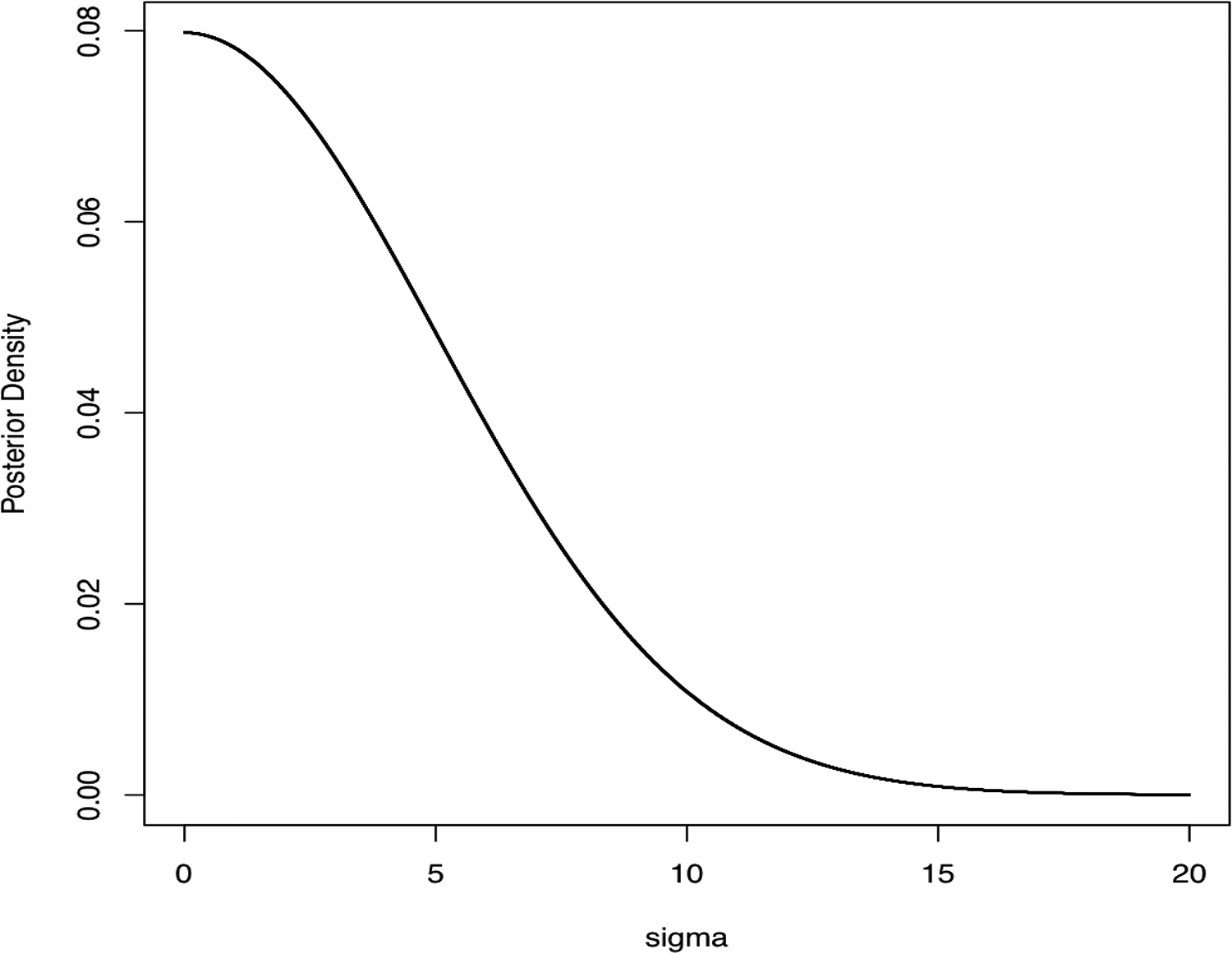
Plot of the posterior distribution of a standard deviation (SD) that shows a mode at the boundary of the parameter space. The 2.5 and 97.5 percentile points would not be a good interval to describe this distribution, nor would the mean and SD.

Point Hypothesis Testing

Testing a hypothesis that a parameter is exactly equal to a specified numerical value (usually zero) would seem to be completely irrelevant to a Bayesian: Most parameters are on a continuous scale (even if the data aren’t), so the probability that a parameter is any particular value, say k, is zero, symbolically p(θ = k) = 0. A Bayesian can only give nonzero probability to a continuously distributed parameter being in an interval, say (a, b). To approach the problem usually of interest in classical hypothesis testing, a Bayesian would normally have to consider the probability that the parameter is “small” in the sense of being in an interval (−d, d), where d is considered small by some standard (as discussed above).

The approach sometimes taken is to deviate from the usual Bayesian approach and adopt a mixture prior, with a certain probability of the parameter being zero, and the rest of the probability spread out continuously over other values. This is hardly ever plausible; one possible exception is extra-sensory perception (ESP). Even when plausible, the results are sensitive to the amount of probability put on the null value, making the results unreliable. If this method is used, the researcher should report sensitivity to the amount of probability put on zero.

Present a Triplot for Primary Quantities of Interest Where Possible

If plots are presented, often it is preferable to include the prior distribution, likelihood, and posterior distribution in one plot; this plot, called the triplot, is the typical Bayesian plot when the prior is informative.

Note that not all prior distributions are reasonable. All informative priors should be checked, and results reported in detail or summarized. Reasonableness of the prior is seen most easily in a triplot, which contains the prior distribution, the likelihood, and the posterior distribution. If the prior is relatively flat in the area of the parameter space where the likelihood is appreciable, then the prior is said to be locally uniform or locally uninformative. If the prior has appreciable mass in areas where the likelihood is (relatively) very low, then the prior is contradicted by the data and should not be considered reasonable (see Albert, 2009; Evans & Moshonov, 2006; Kruschke, 2015; Lunn et al., 2012; O’Hagan, 2004, 2008; Spiegelhalter et al., 2004).

An example of a triplot is shown in Figure 2, which shows plots for a binomial experiment. Notice that in this case, the prior has most of its mass on the left, while the likelihood has most of its mass on the right. The two do not overlap much, indicating a conflict between the prior and the data. Either the prior is inappropriate for these data or the data are inappropriate for this model and prior. In either case, the analyst should note that there is a problem and, if possible, should explore the cause for the discrepancy. An analysis with noninformative priors should be presented for comparison.

OPEN IN VIEWER

Figure 2.

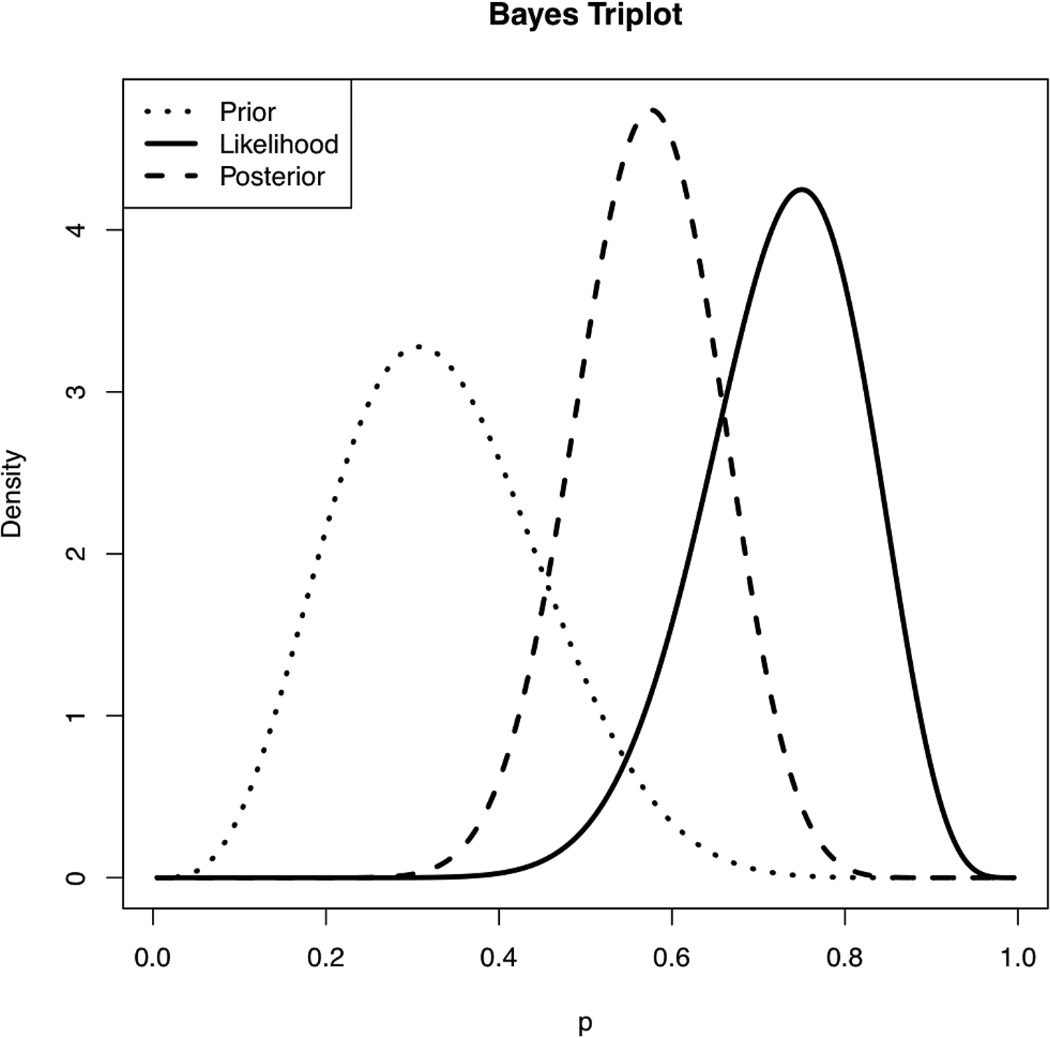
Triplot showing the prior distribution, likelihood, and posterior distribution for a proportion in a case where the prior is inconsistent with the data (likelihood). The prior is a beta(5, 10) distribution, with a mean of .333. The data consist of 15 successes and 5 failures; the observed proportion of successes is .75.

When a triplot is difficult to produce, sometimes a plot of just the prior and posterior distributions will serve reasonably well. In either case, if the prior and posterior are approximately the same, the data are uninformative for the parameter, and this should be reported. As in the triplot, if the prior and posterior modes are inconsistent, there is a problem; perhaps a less informative prior should be considered. At the very least, this should be drawn to the reader’s attention and discussed.

Where prediction is a goal, describe the predictive distribution for future observations

If a prediction or forecast is being made for an observable quantity, the actual distribution and parameter estimates for the predictive distribution should be made available, a set of summary statistics to describe the distribution, or a graphical summary should be provided.

Parameters are unobservable, so one cannot always check whether inferences about them are reasonable. A prediction of observables can be tested. Report all such predictions made on available data either by cross-validation or similar methods. Some methods of checking predictions concentrate on particular aspects of a distribution (e.g., the maximum value); if this is the case, make and report on several predictions that focus on different aspects of possible failure of prediction.

Where decision making is a goal, describe the set of actions and the utility functions used, present sensitivity analyses for different utility functions and the usual sensitivity to priors

In policy contexts, there are typically multiple stakeholders or groups of stakeholders, each of whom would have different utilities. For example, stakeholders might include the federal government, state and/or local governments, and groups of citizens with different utilities. In medical contexts, the patients’ utilities may differ from health care administrators, regulatory agencies, or even the doctors. A full analysis should report sensitivity to different stakeholders’ utilities.

In decision making, one of course must specify the various options for decisions (actions) but must also specify utilities (costs and benefits) of various possible outcomes. The focus is not on parameter estimation, but the optimal decision. The optimal decision may be sensitive to the choice of utilities, so sensitivity analysis is usually necessary. The results may also be sensitive to prior probabilities, so this must be tested with respect to the decision, instead of with respect to the effect on parameters. Bayesian decision theory is discussed in Berger (1985) and Chapter 9 in Gelman et al. (2013).

Report Complications Arising With Multiparameter Models

If important parameters are correlated, the joint distribution should be plotted pairwise or described.

The situation can become more complicated with more than one parameter; how much more complicated depends on the correlations among those parameters. If the parameters are independent or nearly so, then inference can proceed for each as if it were the only parameter, and the methods of the previous section can apply.

For other situations, it is possible that rewriting the model will make the parameters (nearly) independent. It can also make parameters more meaningful. For example, in a simple linear regression, the slope and intercept are often correlated. Centering the predictor removes or greatly reduces that correlation. The same is true for polynomial models: One can use orthogonal polynomials to control the correlations among parameters. Other models with interactions often have similar problems. Models with more than one predictor often have correlations, sometimes high, among the variables, which result in correlated parameters. Many methods have been suggested in classical/frequentist statistics for dealing with these problems (and most have been adapted by Bayesians), including eliminating variables, principal components, factor regression, ridge regression, and informative priors.

As an example, Figure 3 shows a contour plot for two parameters, which illustrates the nature of this potential problem. It looks similar to, and is often caused by, the problem of two highly correlated predictor variables that represent the problem of collinearity in (generalized) linear models. For our purposes, there are two characteristics of this plot that are most important: First, the (unconditional) variance of each parameter is large; both are estimated with little precision. Second, conditional on one parameter, the other is estimated with high precision; the conditional variance is small, so if you knew the value of one, you would know the value of the other with little error. Thus, merely reporting the (univariate) estimates and SEs may be misleading in this case.

OPEN IN VIEWER

Figure 3.

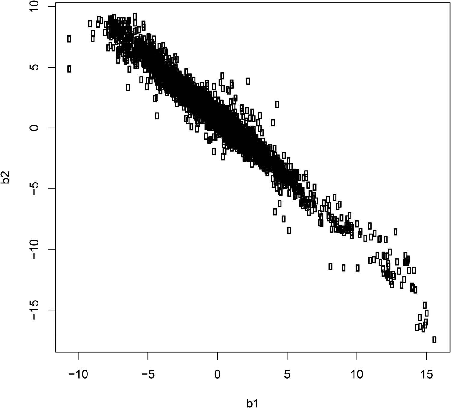
Plot of posterior distribution of two regression coefficients from a highly collinear data set. The unconditional standard error (SE) for each is large, but the conditional SE for each given a value of the other is much smaller.

The problem is more difficult to detect with many parameters, as producing and examining many plots are difficult. With only a few, one could produce a matrix scatterplot, but beyond a handful of parameters, this becomes more problematic. As with collinearity, perhaps the best way to detect this problem is to look for SEs that seem too large for a given sample size. Draw the reader’s attention to any such instances, and describe what (if anything) was done to resolve the issue.

Hierarchical (Multilevel) Models

For multilevel models, explain the rationale for assuming exchangeability (or conditional exchangeability if there are covariates). If it is important to the context, present plots or tables of the shrunken estimates and their confidence intervals.

Hierarchical models are models where one or more sets of parameters in turn have a distribution, requiring the specification of a prior distribution, often known as a hyperprior. In these models, the analyst may additionally be interested in estimating what are, in classical statistics, the random parameters of individual units (e.g., schools, hospitals, work groups) and what are, in classical statistics, fixed parameters. One excellent source (of many) discussing these models is Gelman et al. (2013).

If one of the interests is in estimating random units’ values, these will be what are commonly called shrunken estimates. One of the most useful reporting methods is to present a shrinkage plot, with raw estimates and shrunken estimates plotted in parallel with lines connecting the units across the two lines. An example is in Figure 4. More detailed reporting is sometimes useful, including reporting tables or plotting CIs of shrunken estimates and comparing them to their unshrunken estimates and intervals.

OPEN IN VIEWER

Figure 4.

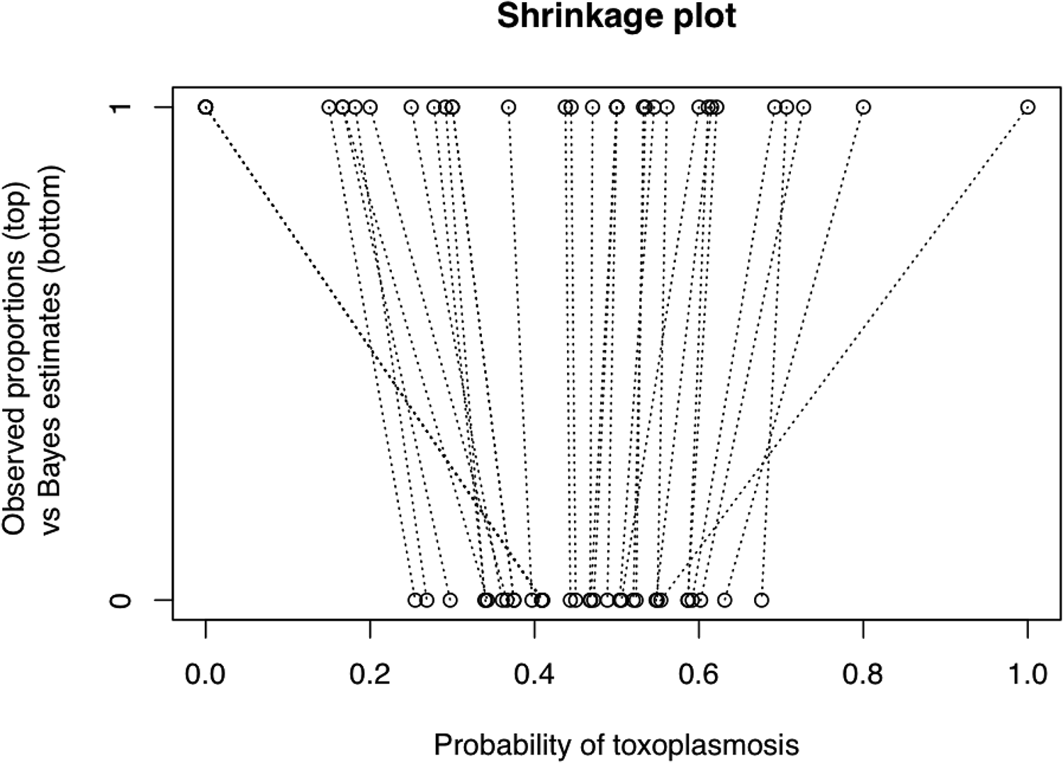
Shrinkage of estimated proportions with toxoplasmosis. Notice that some of the most extreme raw data points are shrunk more than less extreme points, due to very small sample sizes in the extreme points.

If there are few higher level units, then greater care must be exercised. In that case, the variance among these units is not well-estimated, which has implications for the shrinkage estimates. It is useful to present a trace plot (sometimes called a profile log likelihood plot) in these situations: It is a combined plot of the posterior distribution of the SD (often called τ), along with the shrunken estimates plotted as a function of the values of τ. This shows the variability of the shrunken estimates as a function of values of τ that have appreciable posterior probability. Although typically the marginal values of the shrunken estimates are of interest, if there is a large amount of uncertainty about the value of τ, the range of the shrunken estimates is also interesting, and in this case, a trace plot should be provided. (See, e.g., DuMouchel, 1994; Rubin, 1981; Spiegelhalter et al., 2004, p. 97.)

Meta-Analysis

In addition to the usual reporting for multilevel models, forest or caterpillar plots should be provided that include original and shrunken effect size estimates for each study and interval estimates for the quantities of interest. If feasible for the analytic method used, a trace plot (discussed above) should be reported that plots shrunken estimates versus the SD of the residual effects (as in DuMouchel, 1994, Exhibit 3; Rubin, 1981, Figure 2; Spiegelhalter et al., 2004, Figure 3.13).

Meta-analysis is a special case of a hierarchical model in which the observations at the lowest level are not available, but summary statistics (effect sizes) and their SDs (or variances or precisions) are used in the analysis. They therefore inherit some requirements for reporting from the general case of hierarchical models but add some of their own. The trace plot (Hierarchical/Multilevel Models section) showing estimates of effect sizes for each study as a function of the variability among studies, and a histogram of the posterior of that variability, is one of the most useful Bayesian plots. For more details on Bayesian meta-analysis, including examples of displays and plots, see DuMouchel (1994) and DuMouchel and Normand (2000). Similar techniques (and therefore similar reporting methods) are used in institutional comparisons (e.g., death rates from surgery, or average test scores for schools, classes, or teachers in so-called “league tables”).

Adaptive Designs

For adaptive designs, describe the details of all rules for decisions, when these rules were decided (before or during the study), and the consequences (results) of each decision.

Most studies in the social sciences have a sample size fixed in advance. This can be wasteful: A large effect might be easily seen as significant when only a small sample has been collected, obviating the need to test more people. In medicine, not only is this seen as wasteful but also unethical; trials are often stopped before the planned time when one treatment is obviously more efficacious than another. Further, some designs in medicine switch treatment probabilities when one treatment seems (but is not yet proven) to be more effective than another. In some cases, reporting of results is not much more complicated, but reporting the design and analysis and their details takes more care than for simpler designs. All decision rules should be specified, even those that did not occur in a particular study. All decisions that were made should be reported. An important reference for Bayesian adaptive design in clinical trials is Berry et al. (2010).

Computations and Complications With Them

If MCMC or another sampling procedure is used, it should be described in detail: number of chains and, for each chain, the number of burn-in iterations, sampled iterations, and thinning. Describe the methods that were used to check for convergence and their results.

Report Burn-in, and Convergence and Accuracy Checks

Modern computational methods bring with them certain problems that must be addressed in the reporting of Bayesian results to ensure that those results represent the correct posterior distributions. As previously mentioned, these modern methods primarily involve simulation, notably some variation of MCMC methods originally developed by physicists. These methods can be problematic either by causing bias or indeterminacy in estimation, which is fatal (but hopefully rare), or lack or precision, which is merely annoying, and is solvable by running the process long enough. (More complicated models such as mixtures can have yet more problems, beyond those discussed here.)

Simulations using MCMC methods go through two phases: a burn-in, in which the process stabilizes, and a post burn-in phase in which the process has stabilized and gives draws from the posterior distribution. If the burn-in period is too short, the process has not stabilized, and some or all of the draws are not from the posterior. Both to prevent this and to ensure that the process has converged to the right area of the parameter space, analysts often run several computations starting from different parts of the parameter space and observe whether these converge to the same area; each of these computations is called a chain, and often three or four chains are used. All such choices and their results should be reported. Several tests of whether a run has converged are also available, including those of Brooks, Gelman, and Rubin; Raftery and Lewis; Geweke; and Heidelberger and Welch; at least one should be reported.

Report the Accuracy of MCMC Estimates

The MCMC process is efficient to the degree that successive draws from the posterior distribution are independent of previous draws. Analysts should report whether they examined the autocorrelations of various lags, and at what lag the autocorrelations became low. High autocorrelations do not cause bias in estimates but do make it necessary to simulate more data in order to get accurate estimates. The MCMC error is commonly provided by Bayesian software to address this issue. The researcher need not report every value, but if not should at least say how many decimal places of accuracy are attained for important quantities. Alternatively, some programs list the effective sample size (ESS). Reporting the ESS will give the reader important information about the accuracy of the estimates.

Model Assessment, Comparison, and Combination

Describe the procedures used to check the fit of the model (or models) and the results of those checks (and model comparisons). Bayesian specification and model checking have gone through a period of elaboration over the years. Early Bayesian analyses assumed that the one model chosen was the right one and based all inferences on that model. Then, came a period in which models were considered that were expansions of the base model; for example, a negative binomial (gamma-mixed Poisson) as a generalization of the binomial distribution. These expansions paid no attention to the use of the same data more than once and have been replaced by methods such as k-fold cross-validation, bootstrapping, and calibration cross-validation (Draper, 2013) that hold out some data for validation. Other modern approaches try to do away with the restrictive assumptions of particular distributions or functional forms; these result in nonparametric (NP) Bayesian methods. Some of these will be discussed separately, while general principles will be discussed in this section.

Some model checking is the same as for the usual frequentist statistics and will not be discussed. Other tasks are similar in purpose to typical model checking but are done in a different way in the Bayesian context. One of most prominent is called the posterior predictive p value (PPP; Rubin, 1984). This method involves simulating replicate data sets that from the model and computing a statistic on the actual data set and replicates; if the statistic from the actual data set is “unusual” in the context of the statistics produced by the replicates, there is evidence against the model being correct. Because each PPP is typically designed to test only one aspect of the data, the researcher should specify and report a number of such tests to examine different aspects of the model. Report the statistics being used, what they are designed to detect, the number of replicate data sets that are compared to the observed data, and the p values. If any p values indicate problems with the model, either the model should be modified or a sensitivity analysis should be reported showing that the important results are not sensitive to the problem.

A good portion of model checking in a Bayesian context involves a comparison of simpler models with more complex models. Four criteria are commonly used for such model comparisons: Akaike information criterion (or Watanabe–Akaike information criterion), Bayesian information criterion (BIC), deviance information criterion (DIC), and log scores. Some are not usable for certain models because the number of parameters is not straightforward to count (most commonly, there are such issues with hierarchical models and mixture models) and because each method is typically more useful either for prediction or for model selection, but not both (Draper, 2009; Krnjajic & Draper, 2014). For these reasons, a rationale for the method used should be explained.

As examples of problems with measures of fit, the BIC can be used for some types of models but is inappropriate for other types, including hierarchical models and mixture models, because the number of parameters is not as straightforward to calculate as might be expected. The DIC was developed to deal with some problematic situations, such as counting parameters in hierarchical models, but the researcher should determine (and report) whether the DIC appears to be sensible in each specific case (usually a very skewed posterior distribution of a parameter will cause problems even with a simple nonhierarchical model). Normally problems can be detected when pD, the number of estimated parameters, is less than the minimum possible number (or even negative). The researcher should then report any reparameterizations that are done to minimize the problem and the results of that process.

Bayes Factors

If Bayes factors are used, the analyst should specify clearly the models being compared and should present the Bayes factors and an interpretation. Testing sensitivity to priors is particularly important with Bayes factors, as the outcome often depends more on the priors than on the data. In particular, report if unit information priors are used; these avoid some of the problems due to uninformative priors. Kass and Raftery (1995) gave an overview of the uses of Bayes factors.

Bayesian Model Averaging (BMA)

In BMA, the analyst should clearly specify the parameter or function of parameters being estimated and either plot the distribution or list the mean and SD if it is near normal, or list a number of percentiles of the distribution if it is not. Describe how models were generated, and if a reduced set was used for averaging, how the selection was done and which models were used in the averaging.

Bayesians sometimes go beyond the usual process of model comparison, combining different models for purposes of prediction or decision making. In BMA (see Hoeting et.al., 1999), researchers (i) develop a list of all (or a large set of) plausible models, (ii) construct a prior distribution of how likely each model is to be right, (iii) find posterior probabilities of each model being right, and (iv) combine predictions of some useful quantity by averaging the predictions of each model, weighted by the posterior probabilities of each model being correct. For reporting purposes, it is important to document how the list of models was arrived at (how were models generated, and if they were thinned, how the decisions were made). The prior distribution on the probabilities of the models, if not flat, should be described and justified. The posterior probabilities of models should be displayed, and the results of BMA should be compared with the predictions of the best-supported single model.

In some cases related to BMA where there is no quantity being predicted, but model comparison is the desired end (e.g., regression models), the posterior probabilities of the models that are greater than some small amount (e.g., .01) should be reported. In some such applications, the desired outcome is rating each predictor variable on its importance, and in such cases, the researcher may either report for each variable the sum of the posterior probabilities for models containing the variable or plot those probabilities.

Non-Parametric (NP) Bayes

NP Bayes is a recent development and has many promising applications. It is, perhaps, too soon to codify rules for presenting NP Bayesian results. I will outline some reasonable suggestions for one application of NP Bayes. One way to bypass the need to worry about the specification of the form of the prior distribution is to let it be any possible distribution. To allow complete flexibility of the shape of the prior, it is necessary in theory to adopt an infinite dimensional process (in practice, of course, a finite dimensional approximation is used). Typically, the type of process would be specified (usually Dirichlet process or Polya tree), with a prior consisting of a centering distribution and prior sample size. A sensitivity analysis for those specifications should be reported. If these NP methods are used, besides the usual detailed description of the procedure, they should also be compared with the most appropriate parametric model, which may fit just as well and with smaller SEs than the NP version.