



Abstract
The COVID-19 pandemic poses a serious threat to investors in the crude oil market. Furthermore, investors have an increasing need to find a safe haven in their investment portfolios when facing unprecedented risks in crude oil markets during the COVID-19 pandemic. According to a review of the literature, there are contradictory findings on which investment is the safer haven for the oil market. Therefore, this paper aims to evaluate whether bitcoin is a safer haven for the crude oil market than the commonly used gold during the COVID-19 pandemic. Three spillover measurements based on the time, and frequency domains, and a network framework are employed to quantify the return spillover effects among bitcoin, gold and three major crude oil futures markets. We divide the sample into two periods, pre-COVID-19 and post-COVID-19. The results show that bitcoin has a weak safe-haven effect on the crude oil market only over a short period, while gold maintains a good safe-haven ability for crude oil futures across various time horizons (frequencies), both before and after the outbreak of the COVID-19 pandemic. The findings of this study have important implications for policy-makers, crude oil producers and global investors. In particularly, investors cannot ignore the importance of bitcoin and gold in selecting more profitable portfolio policies when searching for safe-haven assets.
Introduction
On March 11, 2020, COVID-19 was declared a pandemic by the World Health Organization (WHO). The COVID-19 pandemic delivered an enormous shock to the global economy and led to the deepest global recession since the Second World War, by far surpassing the recession in 2009 triggered by the global financial crisis (World Bank 2020).
1
The pandemic affected financial markets as well, but its impact has varied in magnitude for different types of commodities. As shown in Figure 1, the price returns of crude oil decreased by nearly 27% between January and June 2020. The West Texas Intermediate (WTI) on the New York Mercantile Exchange (NYMEX) prices tumbled to $19.5 per barrel, falling the bedrock price since 2002. The single most striking observation to emerge from the data comparison was Brent. The per barrel price of the Brent crude plummeted to $−37.63 on April 20, 2020. China’s first oil futures contract, whose trading symbol is SC, began trading with the Shanghai International Energy Exchange (INE) on March 26, 2018; its price reached less than $0.3 per barrel, dropping to the lowest level. Time evolutions for the time series of oil markets returns. Three considered oil futures contracts are Brent, SC and WTI. The sample period for prices (returns) runs from March 26 (27), 2018, to April 26, 2021.
As the most important source of energy worldwide, crude oil has played a prominent role in the global economy (Wei et al., 2017; Li & Wei, 2018; Bai et al., 2019; Chen et al., 2020; Liu et al., 2020; Li et al., 2022). With the financialization of oil commodities, the structure of oil markets has been elevated highly as oil markets are becoming increasingly capitalized (Li et al., 2020a; Liang et al., 2019; Wei et al., 2020b). Therefore, investors have an increasing need to find a safe haven on their investment portfolio when facing unprecedented risks in crude oil markets during the COVID-19 pandemic (Sharma, 2017; Wei et al., 2019; Jefferson, 2020; Li & Dong, 2020; Bai et al., 2021; Liu et al., 2022; Wei et al., 2022a).
Traditionally, gold is considered a safe-haven investment (Ji et al., 2020; Liang et al., 2020b; Mokni et al., 2020; Morema & Bonga-Bonga, 2020; Salisu & Adediran, 2020). The results of Huynh et al., (2020) show that gold can be a good safe-haven instrument due to its independence. Although a vast body of literature has testified to ‘Gone with the Gold’ (Jin et al., 2019; Wei et al., 2020a; Salisu et al., 2020), the safe-haven potential of gold is still time-varying, regime dependent and nonlinear, implying that it varies across different regimes Adekoya et al., (2020). In contrast, some scholars debate that gold and oil markets have become increasingly inefficient in safe-haven assets during the outbreak, which means that gold’s safe-haven properties in the outbreak period have become useless (Mensi et al., 2020).
However, whether bitcoin can replace gold as a safe-haven is also under discussion when investors are sceptical of gold’s safe-haven attributes (Conlon et al., 2020; Corbet et al., 2020; Liang et al., 2020a). Some researchers propose bitcoin as a safe haven for traditional assets for many reasons, including independence from monetary policy, storage of value and limited correlation with traditional assets (Bouri et al., 2016; Stensås et al., 2019; Kliber et al., 2019; Shahzad et al., 2020; Mariana et al., 2021). In contrast, others considering bitcoin as a safe haven are unlikely to be worthwhile (Smales, 2019; Chaim & Laurini, 2019; Geuder et al., 2019; Conlon and McGee, 2020).
More recently, literature that offers contradictory findings on which bitcoin or gold is a safer haven has emerged. The economic impact of the COVID-19 pandemic on the dependence structures between oil and gold prices has not yet been analysed (Bedoui et al., 2019; Wei et al., 2021). Bouri et al., (2020) find that bitcoin’s safe-haven properties are better than those of gold and commodities. In contrast, Dutta et al., 2020), using the DCC-GARCH model, suggest that gold is a safer haven asset than bitcoin for global crude oil markets. Moreover, Thampanya et al., (2020) findings imply that adding gold or cryptocurrency to a stock portfolio does not enhance its risk-adjusted return.
Specifically, it is significant for investors to identify the effective safe-haven assets on crude oil markets in view of the returns on the investment portfolio when the ‘black swan’ events outbreak. Therefore, the main purpose of this study is to evaluate whether bitcoin is a safer haven for the crude oil market than the commonly used gold during the COVID-19 pandemic.
To identify the safe-haven abilities of gold and bitcoin, the concept of a safe-haven asset must first be defined. An asset that is negatively correlated with a main asset during an economic downturn is called a safe-haven asset. The presence of such assets in a portfolio allows possible losses to be overcome under standard market conditions, as well as in times of turbulence (Akhtaruzzaman et al., 2021; Baur & Lucey, 2010; Kliber et al., 2019; Li et al., 2020b).
With regard to methods of measuring safe-haven assets, current research can mainly include the following categories. (1) Static models. For instance, Hasbrouck, (1995) suggests an econometric approach based on an implicit unobservable efficient price common to all markets in measuring price discovery for equities traded on the NYSE and regional exchanges. Anand and Madhogaria, (2012) show the safe-haven ability of gold in situations of dire economic distress by the Granger causality test. However, the static approach takes the form of a single-equation model that fails to describe the variable ordering and dynamic characteristics in the markets. (2) Dynamic models. For example, Joy, (2011) concludes that gold has acted as an effective safe haven against currency risk associated with the US dollar based on a multivariate GARCH model of dynamic conditional correlations. Mariana et al., (2021) also utilize the DCC-GARCH methodology to examine bitcoin and Ethereum as safe-havens for stocks. However, their approach includes dynamic regression and neglects the directionality of information transmission. (3) Other model analysis. Bredin et al., (2015) find that gold acts as a safe-haven asset for a variety of international equity and debt markets for horizons of up to 1 year utilizing wavelet analysis. However, the model does not take into account the investment frequency domain and network analysis.
In terms of safe-haven assets, we find that most of the current studies ignore information transmission, the time–frequency relationship and the network framework relationship between assets and markets. It is crucial to consider these aspects. First, information transmission between assets and the financial market can provide empirical evidence when studying safe-haven assets (Yang et al., 2022; Wang et al., 2022). In addition, considering the frequency can provide strong support for the impact of short-term adjustments, median-term adaptations and long-term policy supervision, which is beneficial for investors to make different choices when connectedness and information transmission vary across time horizons. More importantly, the directional spillover network analysis directly and visually shows that the assets and the financial market act as net spillover recipients or transmitters, which can help investors build suitable investment portfolios with different investment maturities.
Based on the above analysis, this paper employs the connectedness approaches from Diebold and Yilmaz, (2012), Baruník and Křehlík, (2018), and network analysis to evaluate whether bitcoin is a safer haven for the crude oil market than the commonly used gold during the COVID-19 pandemic. The advantages of combining these methods are as follows. (1) The method by Diebold and Yilmaz, (2012) is a well-established approach that is particularly useful in studying information transmission, which appeals to measuring the safe haven of the asset. Moreover, this method solves the problem of researching the spillovers of no more than two markets, such as Granger causality. (2) The Baruník and Křehlík, (2018) method can gain insights into describing the frequency bands (or long-, medium- and short-term horizons) of spillovers, providing a means of estimating the safe haven on the frequency domain. It also avoids the loss of effective information, which is similar to the DCC-GARCH. (3) In view of the network spillover analysis, one advantage of the framework is that it intuitively describes the direction and strength of five markets. Another advantage of using the network is that it is particularly useful in distinguishing the net transmitters and net receivers of a system. (4) The dynamic spillover used in this paper has an important advantage in the evolution of time-varying returns (mainly from four aspects: ‘Total spillover’, ‘Net spillover’, ‘From spillover’ and ‘To spillover’), which allows us to capture gradual and unexpected changes in bitcoin, gold and three crude oil futures and investigate the dynamic spillover effects among markets.
Generally, this study contributes to the research on safe havens during the COVID-19 pandemic. In particular, this study is the first to compare the safe-haven abilities of bitcoin and gold for crude oil markets during the COVID-19 pandemic based on static, dynamic and network perspectives. The empirical results obtained in this work not only demonstrate a return spillover effect in the time and frequency domains but also can help people recognize which market is the main risk transmitter or recipient.
The remainder of this paper is organized as follows. The Evaluation Methodology section is concerned with the methodology. The Data section describes the data. The Empirical Results section presents the findings, focussing on two key themes, namely, static and dynamic analyses. The Robustness Examinations section is concerned with the robustness examinations. The Conclusions section presents the conclusions of this study.
Evaluation Methodology
Spillover Analysis in the Time Domain Using the Diebold–Yilmaz (DY) Method
The process of N-dimensional vector autoregression (VAR) of order


The variance decomposition method measures the proportion of prediction error variance in any endogenous variable affected by different information shocks in the VAR system (Diebold & Yilmaz, 2009, 2011, 2012). It reveals to what extent the trajectory of a variable is due to the impact of itself or other variables in the system. The proportion explained by the variable


The total spillover index

Directional spillover indexes


Traditionally,


Spillover Analysis in the Frequency Domain Using the Baruník–Křehlík (BK) Method
To describe the frequency dynamics (long, medium and short terms) of spillover, Baruník and Křehlík, (2018) consider a spectral representation of variance decompositions based on frequency responses (instead of impulse responses) to shocks. On the basis of the frequency response function

Recent advances in this method facilitate investigation into frequency dynamics.
The generalized causation spectrum can be defined as


The additional condition is that





Similar to Eqs. (6)–(9),

Data
The sample data used in this study consist of three categories, namely, bitcoin, gold and crude oil. Bitcoin is the most popular digital currency, and its daily prices are recorded from the website https://coinmarketcap.com/. The gold price used in this study is the Gold Fixing Price at 10:30 AM (London time) in the London Bullion Market, based on U.S. dollars. Three types of oil markets are selected, namely, the NYMEX-listed West Texas Intermediate (WTI) crude oil market, the Brent crude oil (Brent) market on the London Intercontinental Exchange (ICE) and the Shanghai INE-listed and traded Shanghai crude oil futures (SC).
The markets are selected for the following reasons. On the one hand, current international oil trade is based on three major crude oil quotations. WTI and Brent crude oil futures play the role of benchmark crude oil contracts in North America and Europe, respectively. Since its launch, the daily trading volume of Chinese crude oil futures (SC) has exceeded that of Dubai crude oil futures, becoming the largest crude oil futures contract in Asia and the third largest international oil market (Li et al., 2021; Song & Li, 2015). On the other hand, it is worth noting that SC differs from WTI and Brent in terms of trading hours, product quality, trading geography and currency (Wei et al., 2022b; Zhang et al., 2021). Specifically, SC futures contracts are traded in Chinese yuan (CNY), while WTI and Brent are both traded in US dollars. Trading in Chinese yuan (CNY) not only weakens the pricing control over WTI and Brent to some extent but also facilitates the use of the Chinese currency. Overall, the choice of WTI, Brent and SC as representatives of the crude oil market is useful to study.
Additionally, WTI and Brent crude oil daily prices are collected from the Data Stream, whereas the price of SC is obtained from the Wind Financial Terminal. To enhance the comparability of the data, we initially convert Chinese crude oil futures prices into US dollar-denominated prices through the exchange rate.
2
In addition, the daily returns are computed as
The period selected for analysis in this study is from March 26, 2018, to April 26, 2021. The starting point of the sample period is constrained by the availability of SC data. For improved results, data with inconsistent trading times due to holidays or other factors are excluded, and a total of 735 sample data are obtained. The sample data are further divided into two periods: Period Ⅰ is pre-COVID-19, from March 26, 2018, to January 12, 2020, and period Ⅱ is post-COVID-19, from January 13, 2020, to April 26, 2021. 3
Figures 1 and 2 depict the time series of the returns of bitcoin, gold and crude oil futures over the sample period. Before the outbreak of the epidemic, the yield of the three major crude oil futures changed relatively smoothly. After the epidemic, the volatility was relatively large, particularly from January 2020 to May 2020, after which the volatility was more moderate until August 2020, when it began to fluctuate more volatile again. Before the COVID-19 pandemic, we observed a close dependence on the changes in the returns of bitcoin, gold and the three crude oil futures. In particular, after the COVID-19 outbreak, bitcoin and gold are more closely related. Time evolutions for the time series of Bitcoin and gold returns. The sample period for prices (returns) runs from March 26 (27), 2018, to April 26, 2021.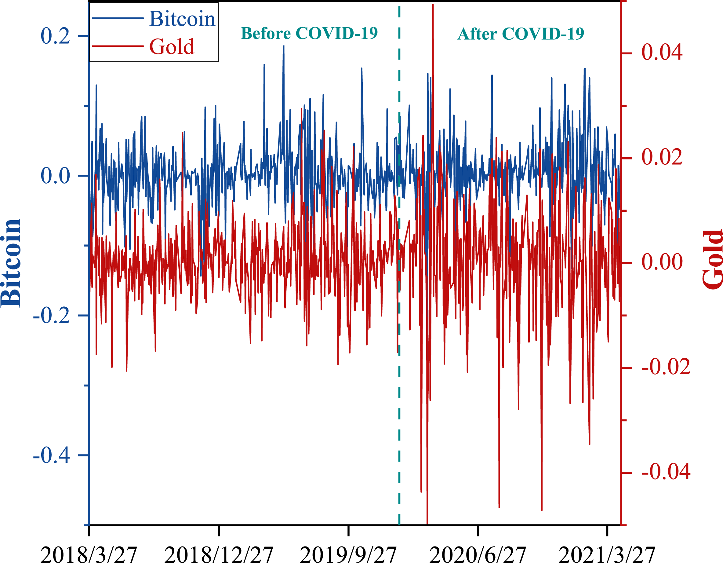
Descriptive Statistics of all Return Series Before the COVID-19 Outbreak.
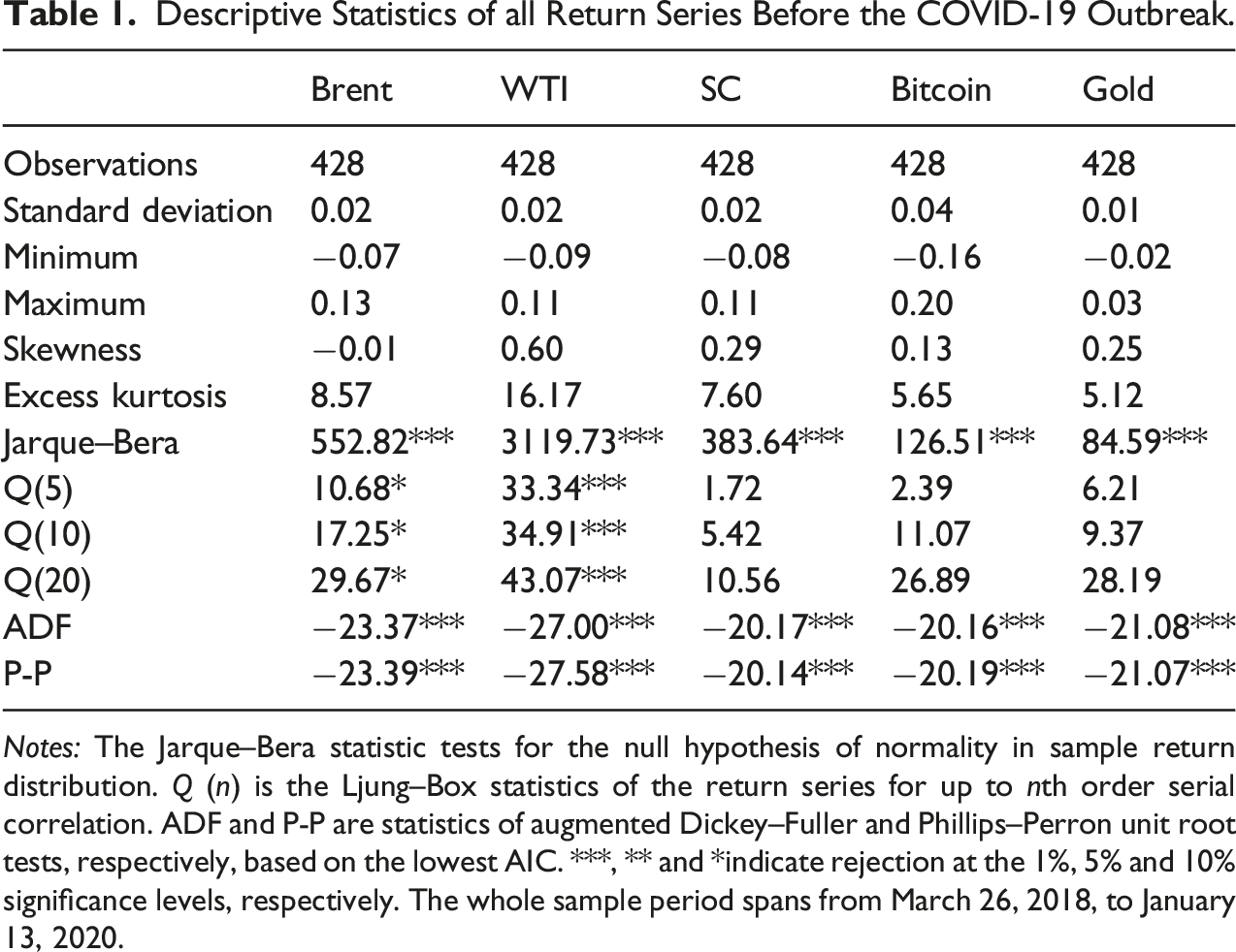
Notes: The Jarque–Bera statistic tests for the null hypothesis of normality in sample return distribution. Q (n) is the Ljung–Box statistics of the return series for up to nth order serial correlation. ADF and P-P are statistics of augmented Dickey–Fuller and Phillips–Perron unit root tests, respectively, based on the lowest AIC. ***, ** and *indicate rejection at the 1%, 5% and 10% significance levels, respectively. The whole sample period spans from March 26, 2018, to January 13, 2020.
Descriptive Statistics of all Return Series After the COVID-19 Outbreak.

Notes: The Jarque–Bera statistic tests for the null hypothesis of normality in sample return distribution. Q (n) is the Ljung–Box statistics of the return series for up to nth order serial correlation. ADF and P-P are statistics of augmented Dickey–Fuller and Phillips–Perron unit root tests, respectively, based on the lowest AIC. ***, ** and *indicate rejection at the 1%, 5% and 10% significance levels, respectively. The whole sample period spans from January 13, 2020, to April 26, 2021.
Empirical Results
Static Analysis Using Full-Sample Spillover Analysis
In the static analysis, we first construct VAR models using the returns of bitcoin, gold, and three crude oil indices in period Ⅰ and period Ⅱ. The lag order of both models is 2 according to the Akaike Information Criterion (AIC). The spillover indexes for the full-sample period are estimated based on 10-day ahead forecast error variance (FEV) decomposition referring to Diebold and Yilmaz, (2012). Then, we mainly analyse the correlation (defined in Eq. (5)) among bitcoin, gold and the three crude oil markets from the time and frequency domains.
Return Spillover Results in the Time Domain.
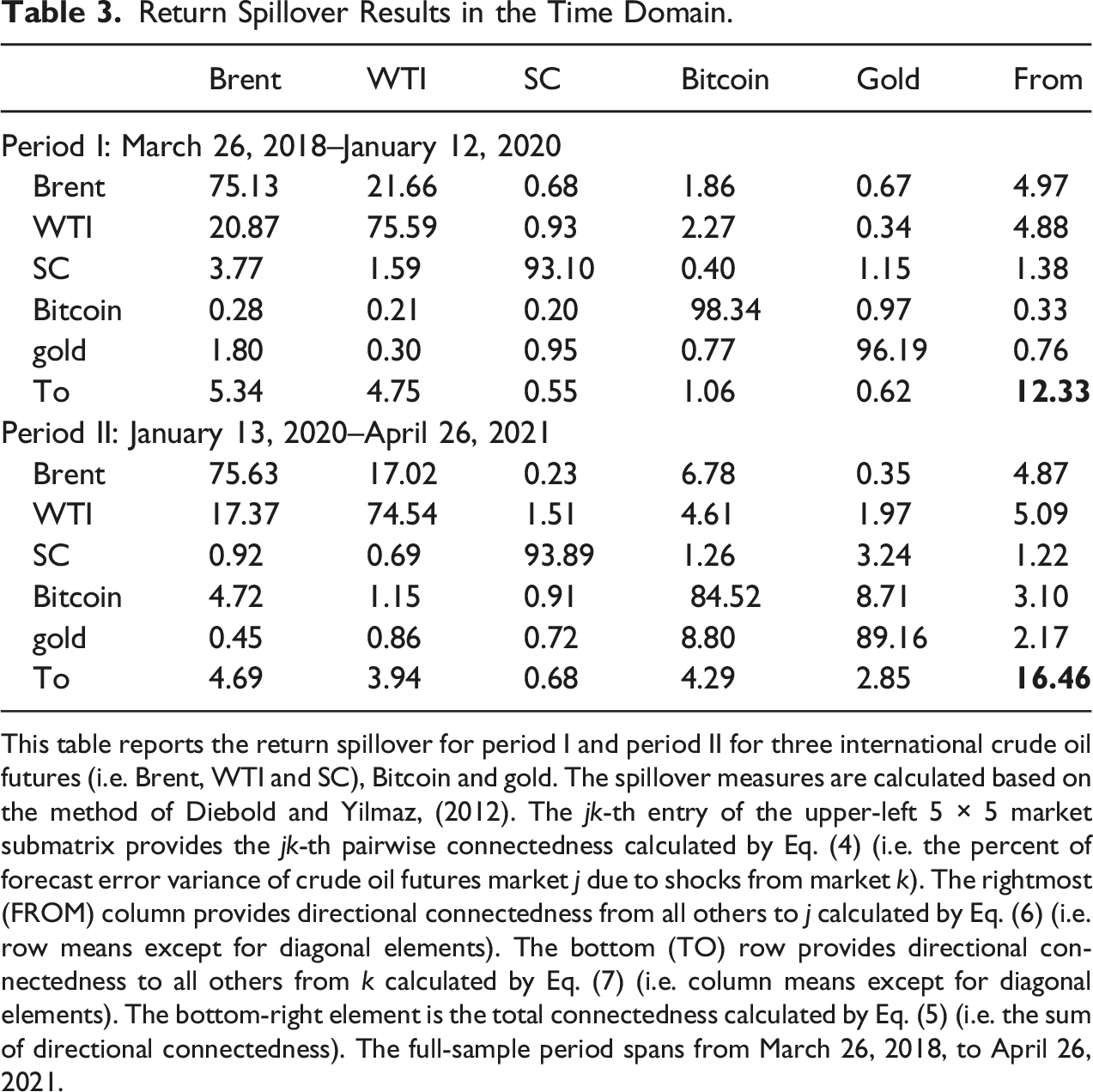
This table reports the return spillover for period Ⅰ and period Ⅱ for three international crude oil futures (i.e. Brent, WTI and SC), Bitcoin and gold. The spillover measures are calculated based on the method of Diebold and Yilmaz, (2012). The jk-th entry of the upper-left 5 × 5 market submatrix provides the jk-th pairwise connectedness calculated by Eq. (4) (i.e. the percent of forecast error variance of crude oil futures market j due to shocks from market k). The rightmost (FROM) column provides directional connectedness from all others to j calculated by Eq. (6) (i.e. row means except for diagonal elements). The bottom (TO) row provides directional connectedness to all others from k calculated by Eq. (7) (i.e. column means except for diagonal elements). The bottom-right element is the total connectedness calculated by Eq. (5) (i.e. the sum of directional connectedness). The full-sample period spans from March 26, 2018, to April 26, 2021.
Overall, the total spillover effect increased from 12.33% before the epidemic to 16.46% after the epidemic. During the epidemic period, the correlation among bitcoin, gold and three crude oil futures markets is enhanced. That is, in this system, the risk of one market is likely to transfer to other markets. Moreover, the correlation between bitcoin and the three crude oil futures markets increased after the outbreak. The spillovers of bitcoin to Brent, WTI and SC increased from 1.86%, 2.27% and 0.40% before the outbreak to 6.78%, 4.61% and 1.26% after the outbreak, respectively. The spillovers of gold to WTI and SC increased from 0.34% and 1.15% before the outbreak to 1.97% and 3.24% after the outbreak, respectively. Thus, bitcoin and gold markets are more closely related to the crude oil market during the outbreak, indicating that investors have the strong choice of liquidity in bitcoin and gold.
Return Spillover Results in the Frequency Domain.
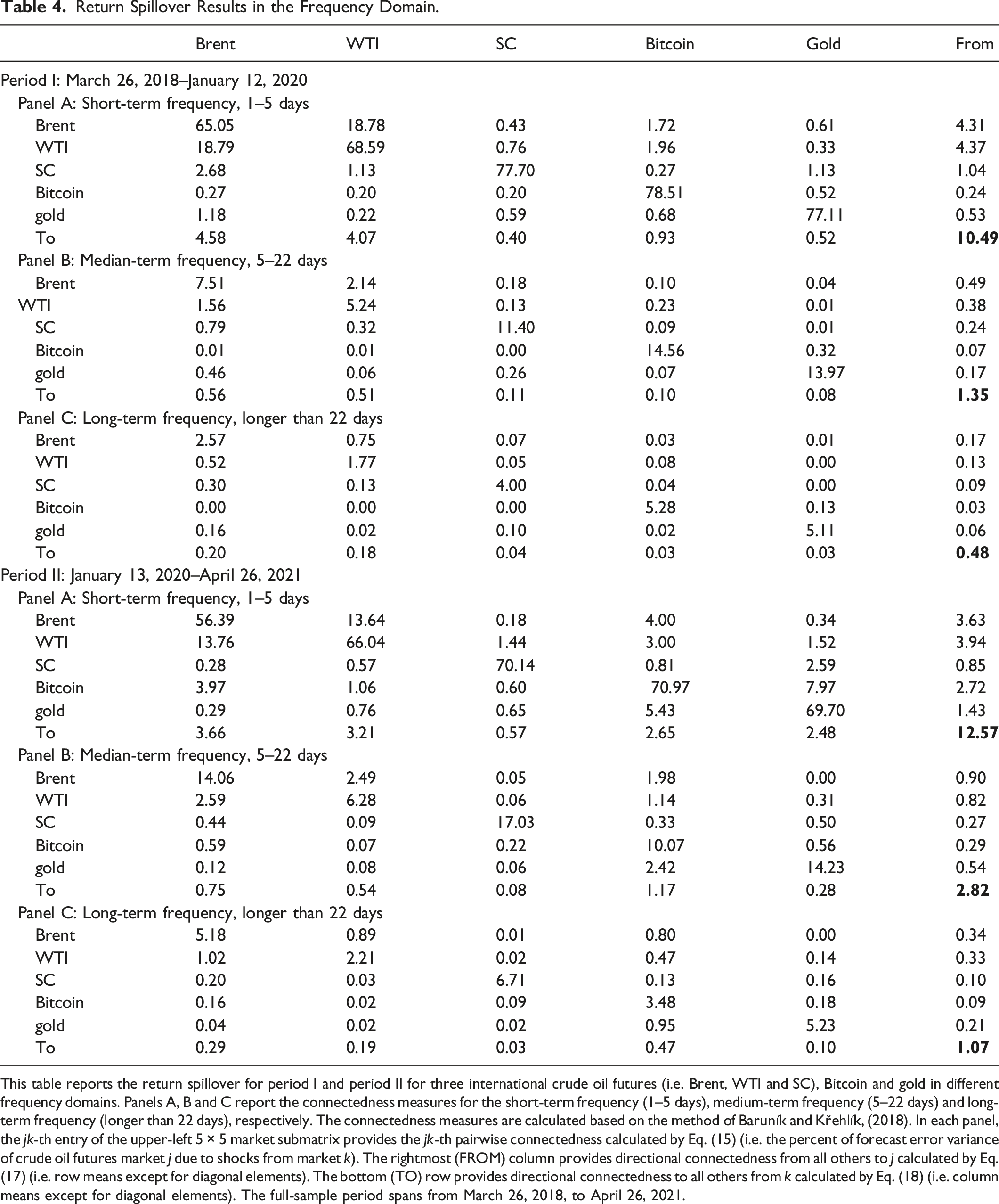
This table reports the return spillover for period Ⅰ and period Ⅱ for three international crude oil futures (i.e. Brent, WTI and SC), Bitcoin and gold in different frequency domains. Panels A, B and C report the connectedness measures for the short-term frequency (1–5 days), medium-term frequency (5–22 days) and long-term frequency (longer than 22 days), respectively. The connectedness measures are calculated based on the method of Baruník and Křehlík, (2018). In each panel, the jk-th entry of the upper-left 5 × 5 market submatrix provides the jk-th pairwise connectedness calculated by Eq. (15) (i.e. the percent of forecast error variance of crude oil futures market j due to shocks from market k). The rightmost (FROM) column provides directional connectedness from all others to j calculated by Eq. (17) (i.e. row means except for diagonal elements). The bottom (TO) row provides directional connectedness to all others from k calculated by Eq. (18) (i.e. column means except for diagonal elements). The full-sample period spans from March 26, 2018, to April 26, 2021.
Before the epidemic, the total spillover effect of the system is 10.49%, 1.35% and 0.48% for the short, medium and long terms, respectively, whereas after the epidemic, the total spillover effect becomes 12.57% (short-term), 2.82% (short-term) and 1.07% (long-term). On the one hand, the spillover after the outbreak is greater than that before the epidemic at each frequency, which is consistent with the results of the DY method. On the other hand, the total spillover decreases from the short term to the long term, whether before or after the epidemic, suggesting that the spillover effect mainly spreads in the short term, and only a few spillover effects spread in the medium and long terms. Thus, in the short term, the relationship among systems is closer, and the return spillover effect is more obvious.
To investigate which market is the net disseminator (or net receiver) during the outbreak, we also calculate the net spillover of each market before and after the outbreak.
The Results of Net Directional Return Spillover Measures.
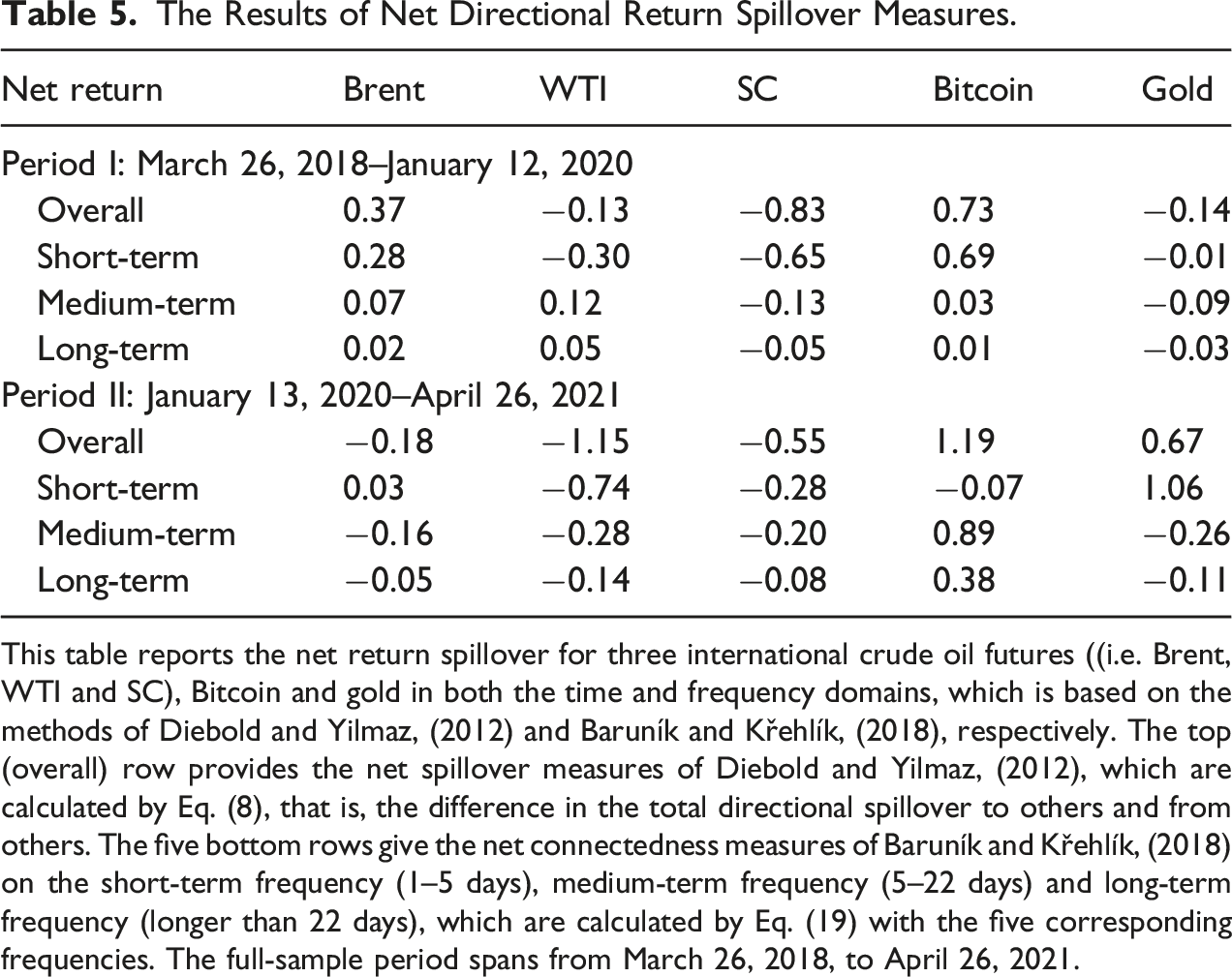
This table reports the net return spillover for three international crude oil futures ((i.e. Brent, WTI and SC), Bitcoin and gold in both the time and frequency domains, which is based on the methods of Diebold and Yilmaz, (2012) and Baruník and Křehlík, (2018), respectively. The top (overall) row provides the net spillover measures of Diebold and Yilmaz, (2012), which are calculated by Eq. (8), that is, the difference in the total directional spillover to others and from others. The five bottom rows give the net connectedness measures of Baruník and Křehlík, (2018) on the short-term frequency (1–5 days), medium-term frequency (5–22 days) and long-term frequency (longer than 22 days), which are calculated by Eq. (19) with the five corresponding frequencies. The full-sample period spans from March 26, 2018, to April 26, 2021.
Network Analysis Using Network Modelling
To better visualize the structure of spillover, we plot the spillover network that specifies the direction and strength of spillover among the five markets. The important parameters are the same as those in the static analysis. Figures 3 and 4 provide the network of pairwise return spillover (defined in Eq. (9)) during press and post-COVID-19. Several important conclusions can be obtained from the network spillover. Directional return spillover network over the pro-COVID-19. Notes: This figure shows the net directional spillover among the Bitcoin, gold and oil markets’ returns. The size of each node indicates the overall magnitude of spillover transmission for each sample, which is measured by pairwise spillover. The thickness of the arrow reflects the strength of the spillover between a pair of variables, with thicker arrows indicating stronger net directional pairwise spillover. Directional-returns spillover network post-COVID-19. Notes: This figure shows the net directional spillover among the Bitcoin, gold and oil markets' returns. The size of each node indicates the overall magnitude of spillover transmission for each sample, which is measured by pairwise spillover. The thickness of the arrows reflects the strength of the spillover between a pair of variables, with thicker arrows indicating stronger net directional pairwise spillover.

Generally, the intersystem spillover effects after the outbreak are greater than those before the outbreak. First, the spillover during the post-COVID-19 period is stronger than that during the pre-COVID-19 period according to a tighter network. Second, after the outbreak, the spillover effect for bitcoin and gold with the three crude oil markets increased significantly. Bitcoin and gold are strongly connected with Brent, WTI and SC. In particular, SC is significantly affected by bitcoin and gold. Third, in view of the three crude oil markets, SC firmly plays the same role. What has changed is that the connection between WTI and Brent weakened. Finally, a weaker spillover network is expected to emerge from bitcoin and gold; however, the relationship between the two has increased after the outbreak (from 0.01% to 0.04%).
Dynamic Analysis Using Rolling-Sample Spillover Analysis
It is widely accepted that spillover effects can vary at any time, and correlations among different markets may increase or decrease under conditions of uncertainty (Sun et al., 2020). However, the full-sample effects are static and represent the average among the five markets, which may overlook any time variation in the spillover effect. Given this, it seems unlikely that any single fixed-parameter model would apply to the full sample. As a result, we study the dynamic spillover effect of markets mainly from four aspects, namely, ‘total spillover’, ‘net spillover’, ‘from spillover’ and ‘to spillover’, based on a 22-day period (contains 1-month observations) with a 10-day forecast horizon referring to Diebold and Yilmaz, (2012).
As shown in Figure 5, at the beginning of the COVID-19 outbreak, the level of short-term risk spillover rose rapidly. Thus, the impact on risk events in the early stage mainly has a short-term influence on each market and aggravates the short-term risk spillover among markets. In March, with the rapid spread of the epidemic, the risk spillover among markets reached the maximum. After May, the spillover effect gradually decreased. The reason may be due to the government’s control of the epidemic situation and people’s understanding and attention to the epidemic situation (e.g. isolation; decreased outdoor activities; and drug research, development and treatment). Dynamic return total spillover. The return ‘Total’ spillover plotted here is computed by the Diebold and Yilmaz, (2011) method of Eq. (5), which is computed based on a 1-month moving window. The sample period for returns is from May 2, 2018, to April 26, 2021.
The time-varying characteristic of net directional return spillover from each market to all other markets is shown in Figure 6. In most cases, the net spillover effects switch to negative and positive territories, suggesting that each market can act as a net or receiver at given points in time. Specifically, in the crude oil market, WTI and Brent show almost the same trend. SC was the opposite; it was negative before the epidemic but became positive after the epidemic. Dynamic return net spillover for sample. The ‘Net’ spillover of returns plotted here is computed by the Diebold and Yilmaz, (2012) method of Eq. (8), which is defined as the difference in the total directional connectedness to others and from others. The dynamic net spillover is computed based on a 1-month moving window. The sample period for returns is from May 2, 2018, to April 26, 2021.
The following conclusions are obtained from Figures 7 and 8. First, the spillover of ‘From’ and ‘To’ have the opposite relationship. The directional spillover almost changes before and after the outbreak. Second, crude oil was greatly affected in April 2020. Finally, at the beginning of the COVID outbreak, especially from January to March 2020, bitcoin and gold show the same trend, but gold is more affected by the outbreak. Thus, gold still maintains a good risk aversion attribute at times of risk. In the short term of risk events, bitcoin also has a certain degree of risk aversion, but compared with gold, it is small. Bitcoin has a little safe-haven effect because it has won the favour of investors due to its convenient trading and high return rates. Dynamic return from spillover for sample. The return ‘From’ spillover is computed based on a 1-month moving window. The sample period for returns is from May 5, 2018, to April 26, 2021. Dynamic return to spillover for sample. The dynamic ‘To’ spillover is computed based on a 1-month moving window. The sample period for returns is from May 2, 2018, to April 26, 2021.

Robustness Examinations
Robustness Analysis by Different Rolling Windows
To establish the robustness of the dynamic results, we employ alternative the three dynamic rolling window sizes of 65-day (one-quarter), 100-day (half-year) and 250-day (1-year) with 10-day forecast horizons, respectively (instead of the 1-month estimates in the Dynamic Analysis Using Rolling-Sample Spillover Analysis section). Then, we also calculate the ‘Total spillover’, ‘Net spillover’, ‘From spillover’ and ‘To spillover’ spanning from the three rolling windows. The following conclusions are obtained.
First of all, as can be seen from Figure 9, it is noticeable that the five markets’ total spillover effects based on three different rolling window sizes (i.e. 65, 100 and 250) increase significantly during the outbreak of COVID-19. More specifically, starting with a lower value of approximately 10%, the total spillover index spike in January 2020 during the pandemic followed a continued decline until April 2021 because of the government’s control of the epidemic situation. Consequently, all these results verify that the spillover indexes follow a similar pattern regardless of the choice of the size of the rolling window, which means that our results are robust and in accordance with the Dynamic Analysis Using Rolling-Sample Spillover Analysis section. Dynamic return total spillover based on different windows. The return ‘Total’ spillover plotted here is computed by the Diebold and Yilmaz, (2011) method of Eq. (5), which is computed based on one-quarter and 1-year moving windows. The sample periods are from July 9, 2018, to August 27, 2018, and April 17, 2019, to April 26, 2021.
Secondly, Figure 10 reports the net directional spillover measure based on three different rolling window sizes (i.e. 65, 100 and 250). Table 6 is organized by the average value of net directional spillover on the basis of Figure 10. The values of the net spillover for gold are always negative both in periods Ⅰ (−0.62%, 0.54% and −0.53%, respectively) and Ⅱ (−0.48%, −0.29% and −0.21%, respectively) with the three different rolling windows, which provides strong evidence that gold remains a safe-haven asset. However, bitcoin has a weak safe-haven effect on the crude oil market when using a 250-day rolling window (−0.11%). Dynamic return net spillover based on different windows. The ‘Net’ spillover of returns plotted here is computed by the Diebold and Yilmaz, (2012) method of Eq. (8), which is defined as the difference in the total directional connectedness to others and from others. The dynamic net spillover is computed based on one-quarter, half-year and 1-year moving windows. The sample periods are from July 9, 2018, August 27, 2018, and April 17, 2019, to April 26, 2021. Dynamic Net Spillover With Different Rolling Windows. Note: The values are produced by the average value of net directional spillover on the basis of Figure 10.

Dynamic From Spillover With Different Rolling Windows.
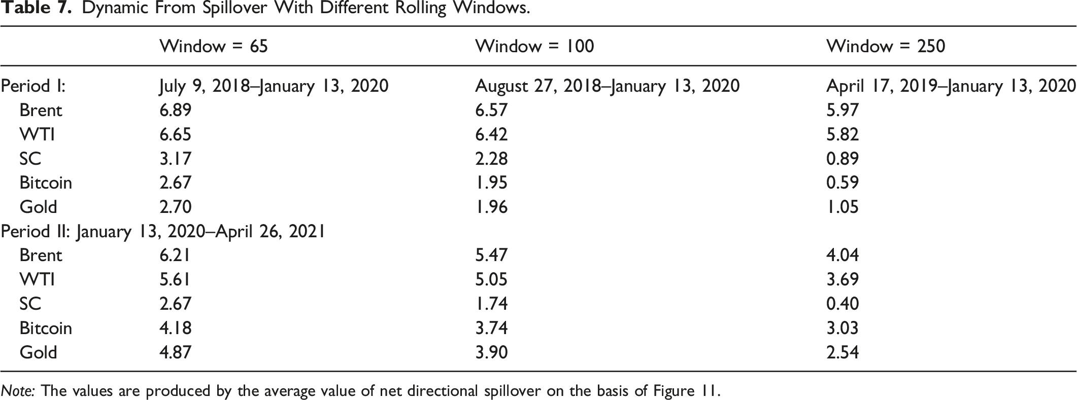
Note: The values are produced by the average value of net directional spillover on the basis of Figure 11.
Dynamic to Spillover With Different Rolling Windows.

Note: The values are produced by the average value of net directional spillover on the basis of Figure 12.
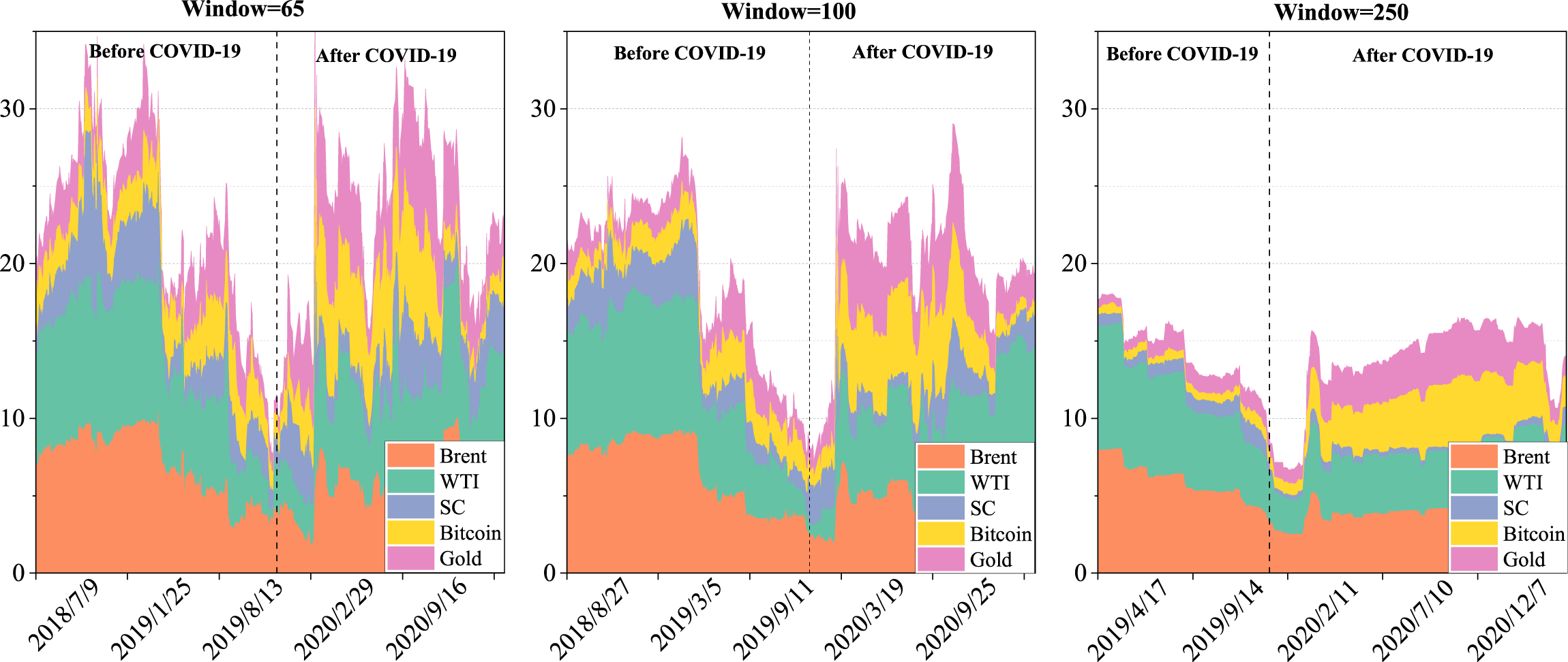
Dynamic return from spillover based on different windows. The dynamic ‘From’ spillover is computed based on one-quarter and 1-year moving windows. The sample periods are from July 9, 2018, to August 27, 2018, and April 17, 2019, to April 26, 2021.
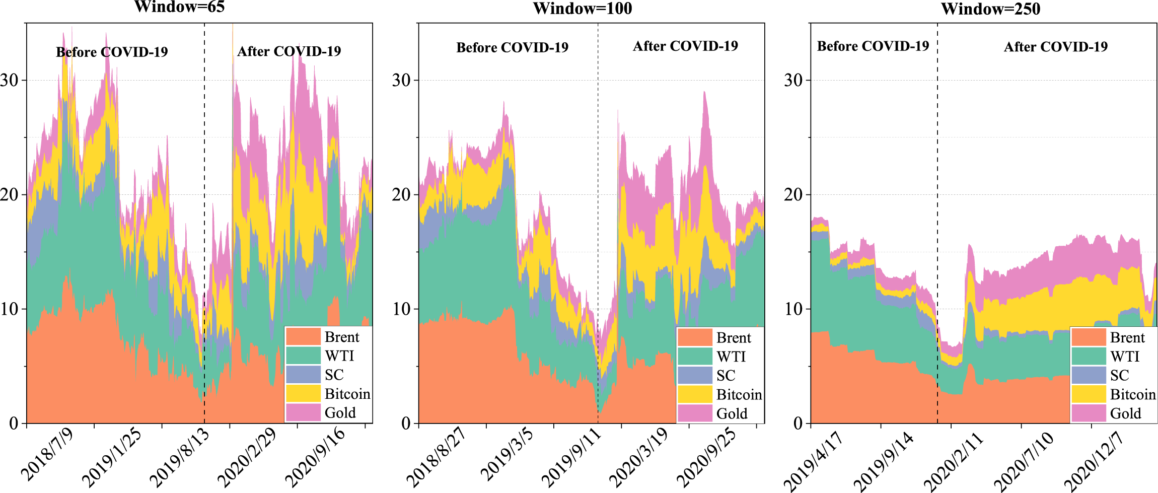
Dynamic return to spillover based on different windows. The dynamic ‘To’ spillover is computed based on one-quarter and 1-year moving windows. The sample periods are from July 9, 2018, to August 27, 2018, and April 17, 2019, to April 26, 2021.
In general, terms, by setting different rolling window sizes, we further confirm the robustness of the conclusions obtained in the Empirical Results section.
Robustness Analysis Based on the TVP-VAR Method
It is instructive at this point to note that the Diebold and Yilmaz, (2012) and Baruník and Křehlík, (2018) VAR-based spillover approaches facilitate the measurement based on the notion of the forecast error variance decomposition from the rolling window. However, the traditional Diebold and Yilmaz, (2012) and Baruník and Křehlík, (2018) methods have not been able to consider small-sample estimation.
In the present study, Antonakakis et al., (2020) provide an extension to the Diebold and Yilmaz, (2012) connectedness approach by applying a time-varying parameter vector autoregressive model (TVP-VAR) with a time-varying covariance structure, as opposed to the constant-parameter rolling window VAR approach. This methodology improves the seminal approach in several ways, such as the fact that no observations are lost as no rolling window is employed, there is no need for choosing an arbitrarily sized rolling window and it overcomes outlier sensitivity. Furthermore, Chatziantoniou et al., (2021) introduce the novel TVP-VAR frequency approach, which is predicated upon previous work by Baruník and Křehlík, (2018) and Antonakakis et al., (2020). Henceforth, we write down the two methods as TVP-VAR-DY and TVP-VAR-BK, respectively. Consequently, we choose the TVP-VAR-DY and TVP-VAR-BK methods to re-estimate the empirical results, which is one of our alternative robustness checks.
Dynamic analysis using the TVP-VAR-DY method
The Results of Average Return Spillover Based on the TVP-VAR-DY Method.
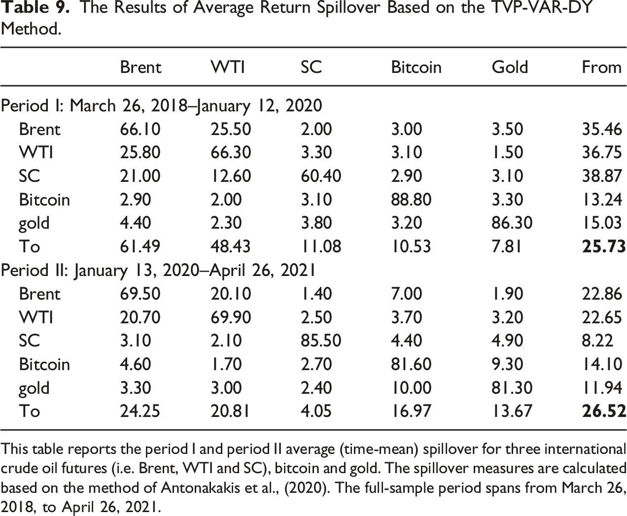
This table reports the period Ⅰ and period Ⅱ average (time-mean) spillover for three international crude oil futures (i.e. Brent, WTI and SC), bitcoin and gold. The spillover measures are calculated based on the method of Antonakakis et al., (2020). The full-sample period spans from March 26, 2018, to April 26, 2021.
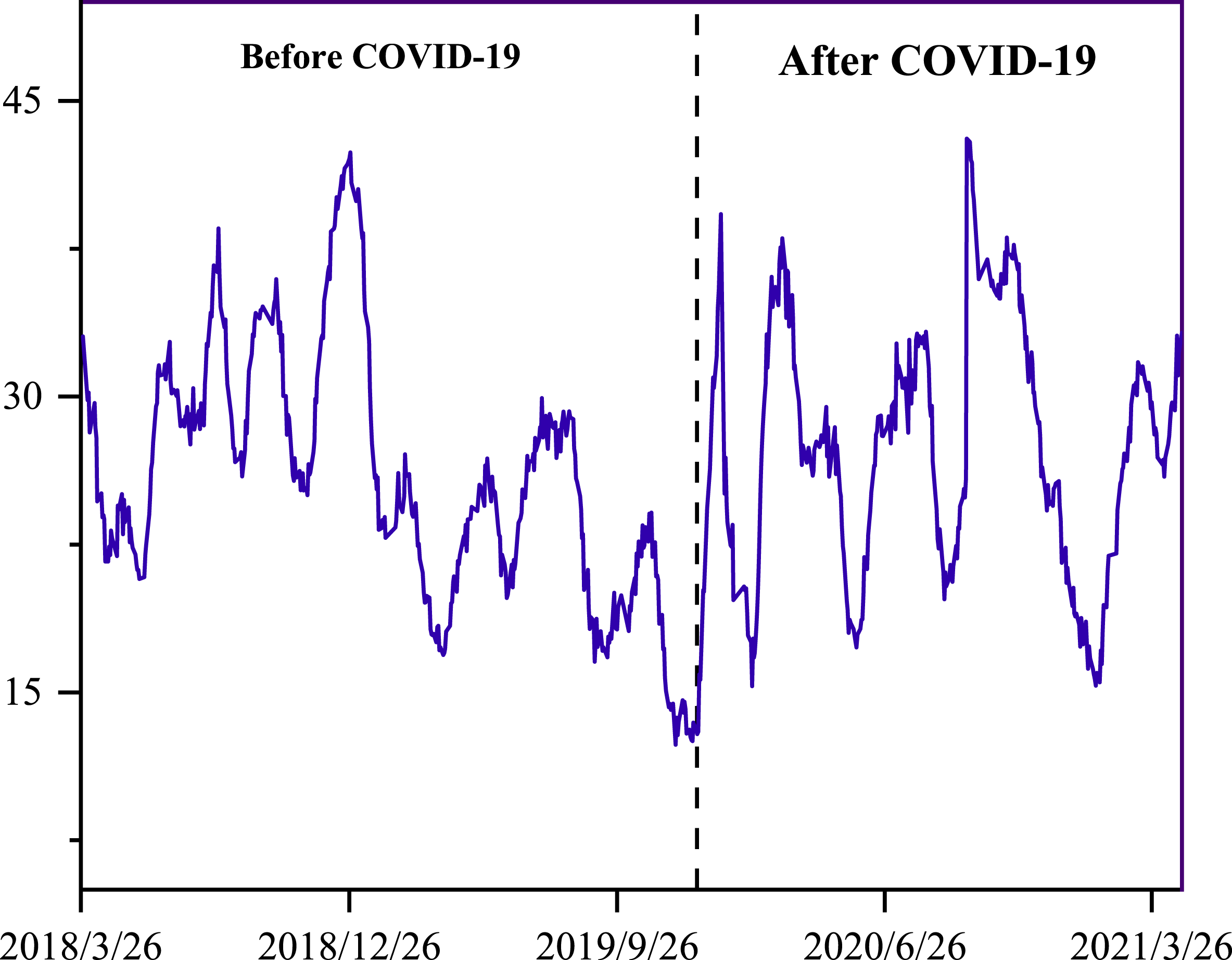
Total spillover of sample returns based on the TVP-VAR-DY method. The sample period for returns is from March 26, 2018, to April 26, 2021.
Moreover, Figure 14 depicts the time-varying evolution of net directional spillovers among the five markets. We can identify the transmitter or the recipient of the net directional spillovers even though the net directional connectedness oscillates in either a negative or positive direction, while their magnitudes often change over time. Consistent with the results in Figure 6, the net spillover results show that WTI and SC oil act as net spillover recipients, while Brent is the net transmitter. Net spillover of sample returns based on the TVP-VAR-DY method. The sample period for returns is from March 26, 2018, to April 26, 2021.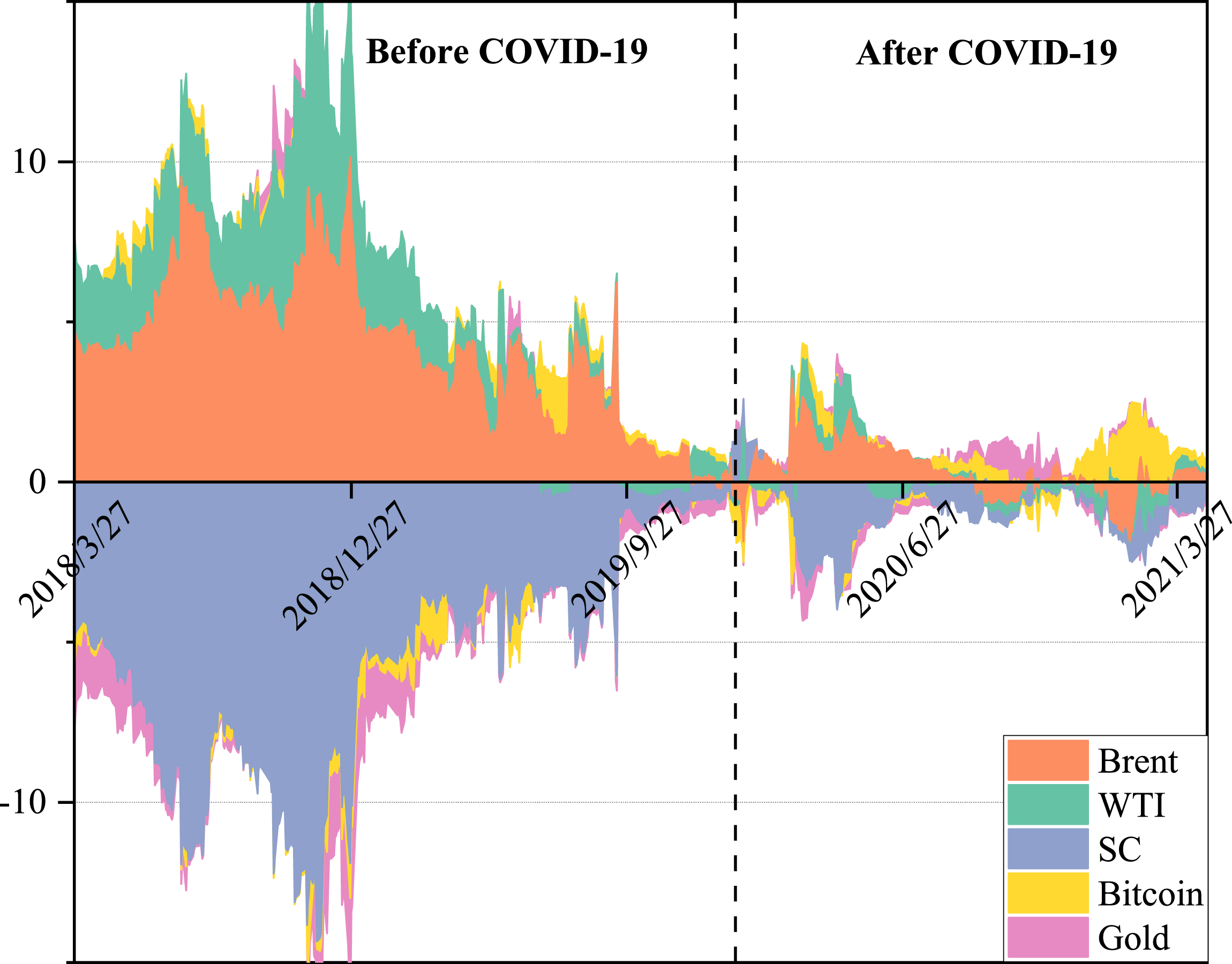
In addition, Figures 15 and 16 present the time-varying ‘From’ and ‘To’ spillover estimated by the TVP-VAR-DY method of Antonakakis et al., (2020). Note that in Figures 7 and 8, the values of spillover are leptokurtic and incomplete. In contrast, the results shown in Figures 15 and 16 are not only smooth but also persistent. It reveals the advantage of a TVP-VAR-based connectedness over the traditional VAR-based approach by its insensitivity, and no observations are lost in the data sample. From the spillover of sample returns based on the TVP-VAR-DY method. The sample period for returns is from March 26, 2018, to April 26, 2021. To spillover of sample returns based on the TVP-VAR-DY method.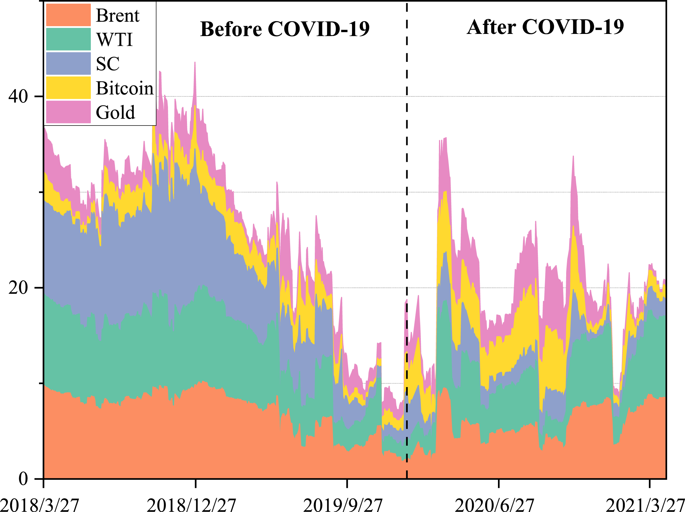

Dynamic Analysis Using the TVP-VAR-BK Method
In the first place, Figure 17 describes the total spillover in the short term (i.e. 1–5 days), the median term (i.e. 5–22 days) and the long run (i.e. longer than 22 days) based on the TVP-VAR-BK method. It should also be noted that the value total spillover is rising extremely fast when COVID-19 occurred. More particularly, the dynamic total average spillover is approximately 10% during phase Ⅰ in the short term, while it is 30% during the COVID-19 outbreak, demonstrating a relatively stronger information spillover in the short term. These findings practically confirm the analysis in the Empirical Results section and provide a more granular picture of the evolution of spillover over time. Total spillover of sample returns based on the TVP-VAR-BK method.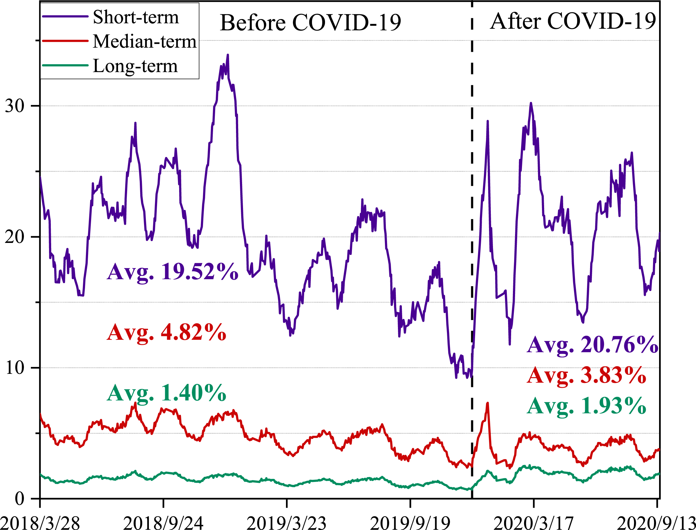
The Results of Average Net Directional Return Spillover Based on the TVP-VAR-DY and TVP-VAR-BK Methods.
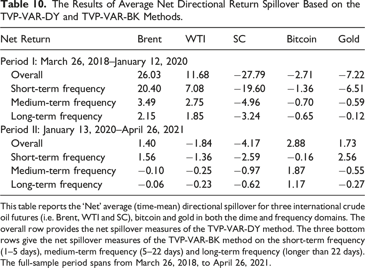
This table reports the ‘Net’ average (time-mean) directional spillover for three international crude oil futures (i.e. Brent, WTI and SC), bitcoin and gold in both the dime and frequency domains. The overall row provides the net spillover measures of the TVP-VAR-DY method. The three bottom rows give the net spillover measures of the TVP-VAR-BK method on the short-term frequency (1–5 days), medium-term frequency (5–22 days) and long-term frequency (longer than 22 days). The full-sample period spans from March 26, 2018, to April 26, 2021.
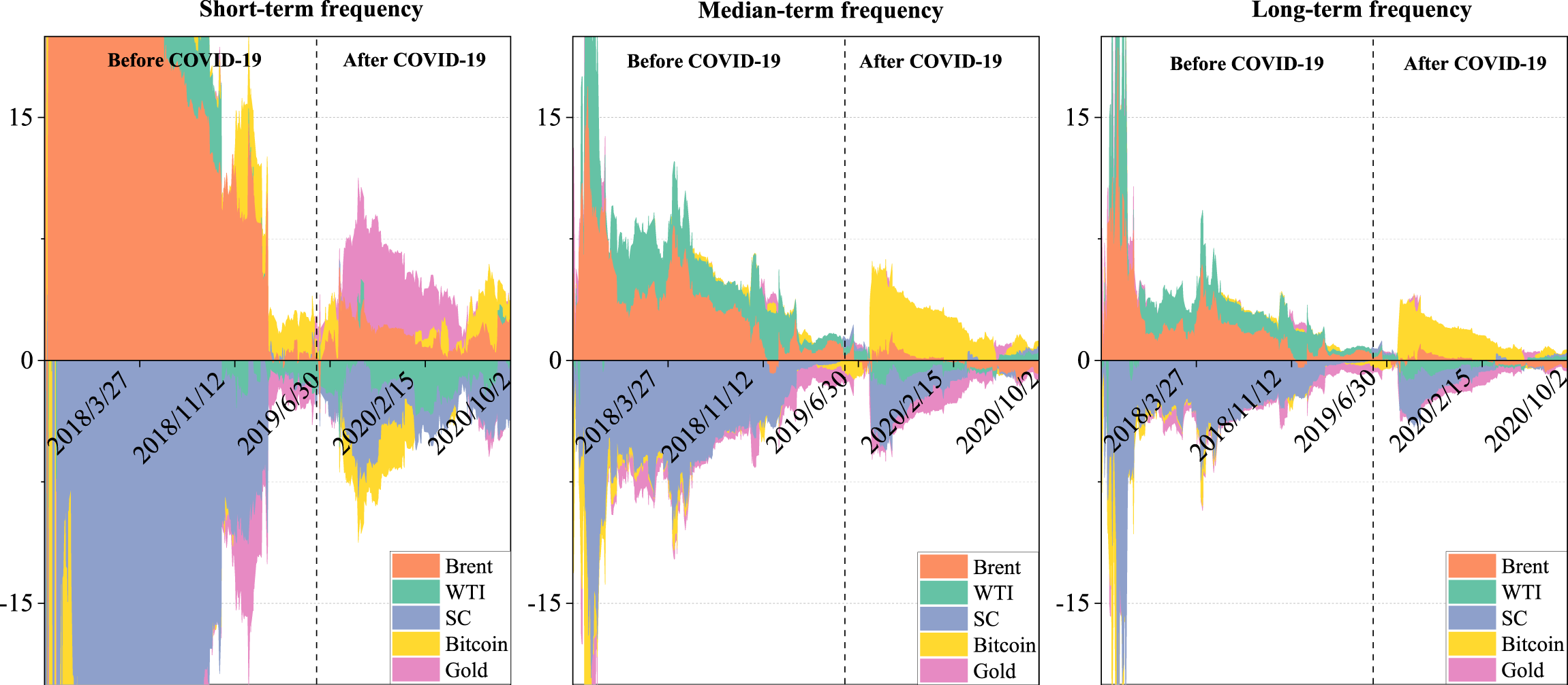
Net spillover of sample returns based on the TVP-VAR-BK method.
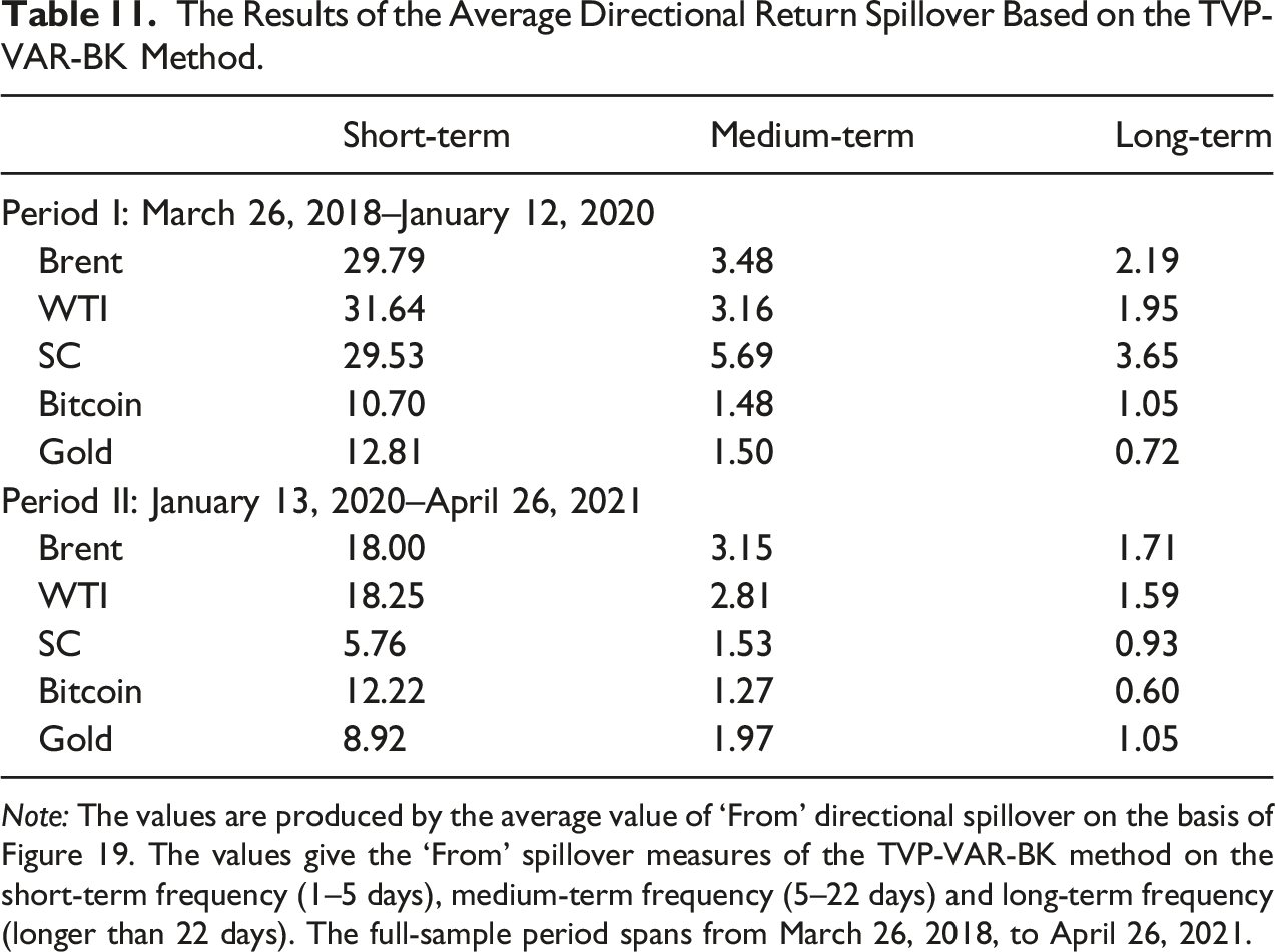
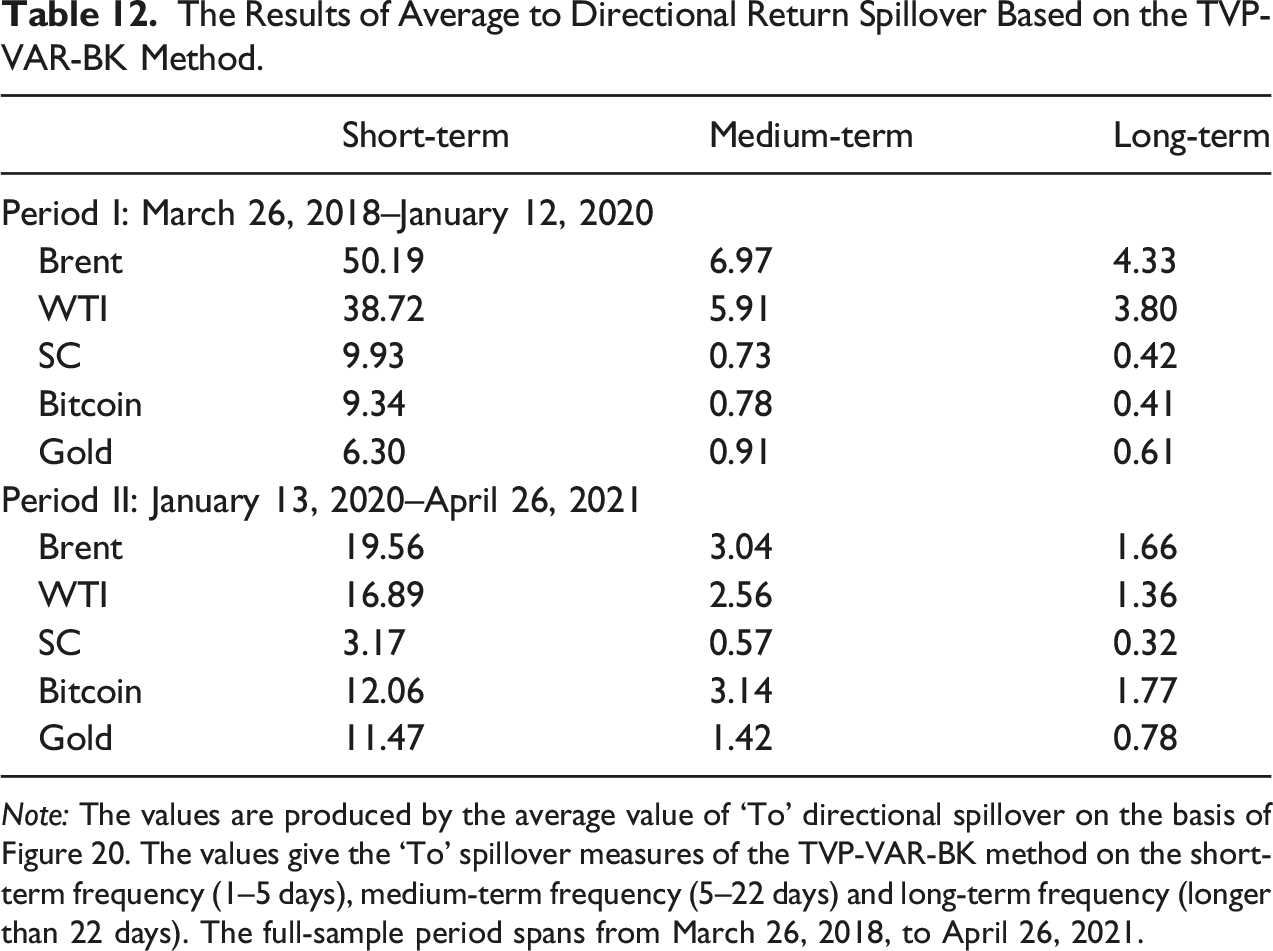
Finally, Figures 19 and 20 further indicate the ‘From’ and ‘to’ spillovers using TVP-VAR-BK, and Tables 11 and 12 are ordered by the mean value of the figures, respectively. Interestingly, the dynamic ‘From’ spillover and ‘To’ spillover measures are ranked as follows: short-term>median-term>long-term. In comparison with Table 4, Figures 7 and 8, it becomes clearer that the dynamic ‘From’ spillover and ‘To’ spillover can be seen in different time frequencies spillover among bitcoin, gold and three crude oil futures markets, again confirming the major evidence found in the Empirical Results section. From the spillover of sample returns based on the TVP-VAR-BK method. To spillover of sample returns based on the TVP-VAR-BK method. The Results of the Average Directional Return Spillover Based on the TVP-VAR-BK Method. Note: The values are produced by the average value of ‘From’ directional spillover on the basis of Figure 19. The values give the ‘From’ spillover measures of the TVP-VAR-BK method on the short-term frequency (1–5 days), medium-term frequency (5–22 days) and long-term frequency (longer than 22 days). The full-sample period spans from March 26, 2018, to April 26, 2021. The Results of Average to Directional Return Spillover Based on the TVP-VAR-BK Method. Note: The values are produced by the average value of ‘To’ directional spillover on the basis of Figure 20. The values give the ‘To’ spillover measures of the TVP-VAR-BK method on the short-term frequency (1–5 days), medium-term frequency (5–22 days) and long-term frequency (longer than 22 days). The full-sample period spans from March 26, 2018, to April 26, 2021.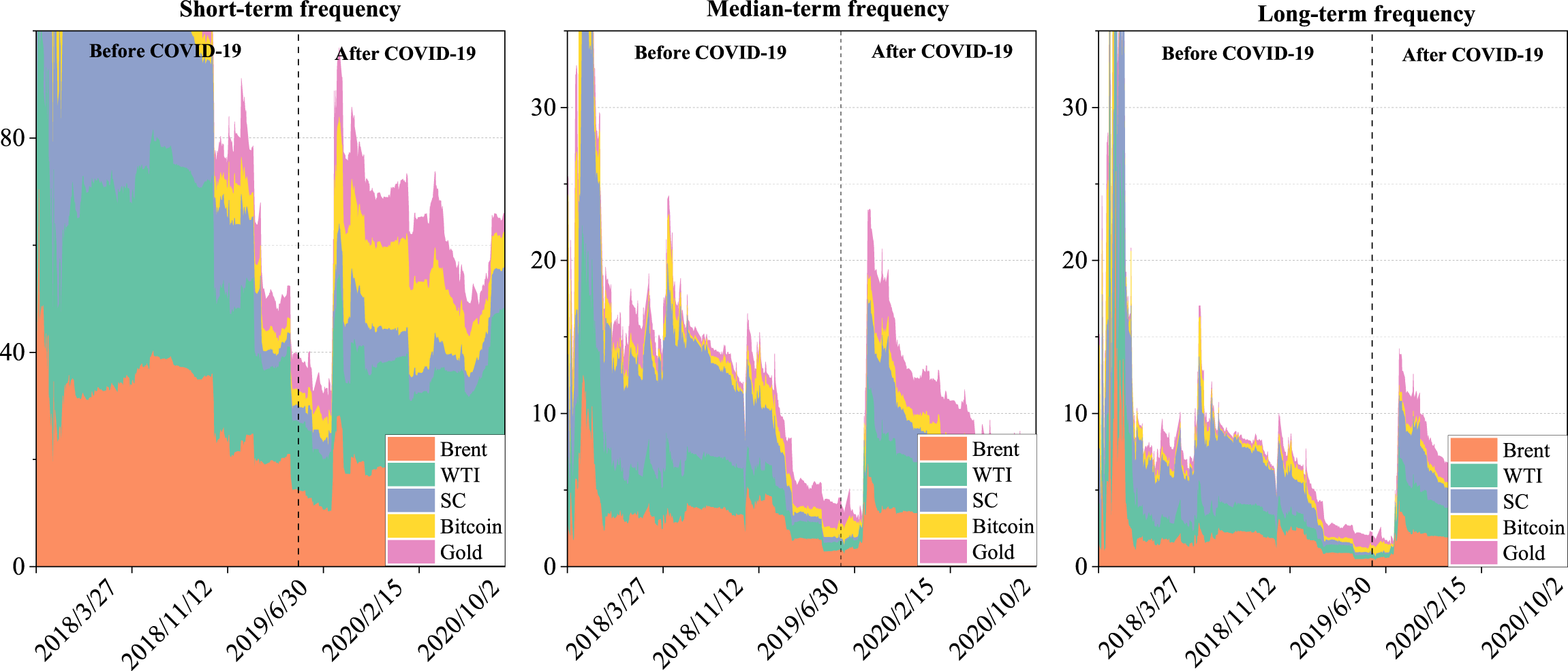

Conclusions
The COVID-19 outbreak has brought strong shocks to a range of crude oil markets. The main goal of this study was to determine whether bitcoin or gold provides investors with an effective safe-haven instrument for the oil market during the COVID-19 pandemic. Our empirical results obtained in this paper demonstrate that, first, the static connectedness measurements reveal that the five markets’ total spillover effect increases significantly after the COVID-19 outbreak, demonstrating a relatively strong information spillover among the bitcoin, gold and three major crude oil futures markets. Specifically, in the time domain, the total spillover effect increased from 12.33% before the epidemic to 16.46% after. In the frequency domain, the total spillover is much larger in the short term (Period Ⅰ: 10.49%; Period Ⅱ: 12.57%) than in the medium (Period Ⅰ: 1.35%; Period Ⅱ: 2.82%) and long terms (Period Ⅰ: 0.48%; Period Ⅱ: 1.07%), implying that a range of shock spillovers for crude oil markets from the outbreak of COVID-19 are mainly transmitted in the short term and just a few spillovers are transmitted in the medium and long term. Then, the directional spillover network analysis directly and visually shows that WTI and SC act as spillover net recipients, whereas Brent is the spillover net transmitter. Finally, all the static and dynamic analysis measurements demonstrate that bitcoin has a weak safe-haven effect on the crude oil market in the short term, while gold always maintains a good safe-haven ability for crude oil markets across various time horizons (frequencies), either before or after the outbreak of the COVID-19 pandemic.
The findings of this study have important implications for policy-makers, crude oil producers and global investors. Given the strong spillover effects among bitcoin, gold and crude oil markets, policy-makers, crude oil producers and global investors need to keep an eye on the spillovers transmitted from other markets when making decisions. In addition, according to the variation rule of the spillover in the frequency domain, investors can adopt the strategy of ‘buying short’ or ‘selling long’ positions to gain benefits. Moreover, the significant effect of the pandemic on the dynamic spillover among the bitcoin, gold and three major crude oil futures markets implies that policy-makers and global investors should consider the factor of ‘Black Swan’ factor in analysing the oil-bitcoin and oil-gold relationships. Last but not least, investors cannot ignore the importance of bitcoin and gold in selecting more profitable portfolio policies when searching for safe-haven assets.
Footnotes
Declaration of Conflicting Interests
The author(s) declared no potential conflicts of interest with respect to the research, authorship, and/or publication of this article.
Funding
The author(s) disclosed receipt of the following financial support for the research, authorship, and/or publication of this article: The authors are grateful for the financial support from the National Natural Science Foundation of China (71971191, 72261034), Science and Technology Innovation Team of Yunnan Provincial Universities (2019014) and Yunnan Fundamental Research Projects (202001AS070018), Yunnan Education Department Scientific Research Fund Project (2022Y478).
