Exchange Rate Models and the Management of Forex Losses in Ghana: Modelling Exchange Rate Volatilities for Businesses

Abstract

Using the Self-exciting Threshold Autoregressive Model (SETAR_M) and linear models such as the vector error correction model (VECM), and univariate models, this article specifies forecasting models for exchange rate volatilities in Ghana and compares their forecasts accuracy using Diebold–Mariano and Pesaran-Timmermann tests statistics. The relevance of this research is to equip business owners and businesses on managing forex losses and to reduce their impact on profits, productivity and employment in high volatile and unstable currency environments. The research concludes that the non-linear SETAR model is superior to the linear models in predicting short-term volatilities in exchange rates, while the fundamentally based linear model is superior for predicting long-term volatility in exchange rates. Therefore, short-term business commitments or transactions such as raw material purchases, cash expenses or incomes in foreign currencies should be planned or managed using SETAR or a non-linear model, whereas long-term contractual obligations like futures and forward contracts should be planned with a fundamentally based multivariate linear model.

Keywords

Ghana exchange rate ARIMA models SETAR model VAR models forecasting accuracy

Introduction

Exchange rates have a significant influence on production decisions and investment plans, as well as on the countries’ prices and competitiveness. Ghana’s exchange rates have been marred with frequent fluctuations leading to loss of business confidence, and obstructions in monetary policy transmissions (Abdul-Rasid & Yao, 2018; Abradu-Otoo et al., 2003; BoG, 2017). Mensah et al. (2013) revealed that exchange rate volatilities have substantially impeded employment growth in the manufacturing sector of Ghana, and it is one of the most unstable rates in the sub-region. To protect businesses and stop the decline in the macro economy, many researchers have proffered improvement in the macroeconomic fundamentals, increased policy transparency and the independence of monetary authorities (BoG, 2017). While these recommendations are likely to stabilize the macro-economy over the long term, businesses in the micro-sector need to manage the short-term effects of the transformational phase on business profits, productivity and employment. For this purpose, businesses, mostly affected by exchange rate volatilities, should have in their toolkit a framework or model which will assist them in planning and predicting exchange rates. The objective of this article is to specify forecasting models for exchange rate volatilities in Ghana and also to compare the forecast accuracy of these alternative models. The absence of this kind of research in Ghana will increase forex losses and put pressure on business profits, productivity and employments. These will result in hyperinflation and a high cost of living in the country.

The literature on specifying or modelling the volatilities in foreign exchange is vast and significant to reducing losses in the forex market (Abbate & Marcellino, 2014). Many researchers have classified these literatures into fundamentally based models and random-walk models. The fundamentally based models are exchange rate models specified or modelled on macroeconomic variables. These models could either be univariate models or multivariate models. The plethora of exchange rate models in research has shifted the focus of recent empirical works to comparing the statistical prediction of the models. For example, Rossi (2013), Carriero et al. (2009) and Cheung et al. (2005) compared the mean square forecast errors of fundamentally based models and random-walk models. The comparison revealed that the fundamentally based models are statistically superior to the random-walk models. This finding, however, contradicts the investigation in Abbate and Marcellino (2014) which supports the superiority of the random walk models over the fundamentally based models. These varying results have led Hauner et al. (2011) to conclude that there is no one superior model and that these mixed results or outcomes are due to differences in economic structures of countries. It is for this reason that Bléjer et al. (2000) emphasized for a country-specific study of exchange rate models rather than a panel study of the problem. Also, Petruccelli and Davies (1986) and Tsay (1991) have drawn a comparison between the linear and non-linear models and found that the non-linear models, as against linear models, are able to capture the dynamics and time irreversibility of a time series better than the linear models. Researchers such as Lee and Chen (2006), Sarno et al. (2004), Granger and Andersen (1978), Maravall (1983) and Tong (1983) have all written extensively on the superiority of the non-linear models in forecasting time series data. Therefore, researchers appear to build consensus on the superiority of non-linear models in forecasting exchange rate volatilities over all class of linear models. Accordingly, this article also intends to model exchange rate volatilities using Ghanaian data and to compare the forecasts or predictions of competing models. The approach adopted in many research works on this topic has been to employ traditional tools such as the mean square errors (MSEs) to compare between the forecasts of different models. These tools are, however, heavily criticized for their lack of economic meaning and unreasonable forecasts (Granger & Pesaran, 2000; Pesaran & Skouras, 2002). This research, besides using the MSEs, also employs Diebold–Mariano (DM) test statistics and the Pesaran-Timmermann (PT) test statistic to compare the forecast performance of the competing models. This approach ensures that business owners and businesses are able to manage (with minimum forex losses) the increasingly unstable and volatile currency in the country.

The objective of this article is to specify forecasting models for exchange rate volatilities in Ghana, and also to compare the forecasts accuracy of competing models. The research concludes that the non-linear model is superior to the linear models in predicting short-term volatilities in the exchange rate, whereas the linear model (the fundamentally based model) is superior for predicting long-term volatility in exchange rates. This result confirms the assertion in Abbate and Marcellino (2014) that the linear models added with macroeconomic differentials have higher predictive likelihoods at long horizons and during periods of recession. Therefore, short-term business commitments or transactions such as raw material purchases, cash expenses or incomes in businesses should be planned or managed using SETAR or a non-linear model, whereas long-term contractual obligations like futures and forward contracts should be planned with a fundamentally based multivariate linear model. The research also made recommendation for future research into determining the avoidable forex losses in the financial statements of a panel of businesses using the conclusions in this research.

The rest of this article is organized as follows: The second section is on the literature review, the third section is the methodology of the study, the fourth section is results and discussions, and the fifth section is conclusions.

Literature Review

This research studies one of the most volatile currencies, which have undergone several redenomination in Africa. The most recent redenomination that marks the start of the third cedi regime from 2007 has led to the taking off of four zero digits that brought the Ghana cedi on equal footings with the pound sterling of the fourth phase (Bank of Ghana Statistics and Reports Office, 2018). These exercises made Ghana cedi the highest denominated currency unit issued in Africa by 2007. The decision to redenominate the currency was to ensure ease of carrying the cedi. The redenomination did not have much to do with the value of the cedi relative to other currencies. Therefore, the ‘free fall’ of the cedi continued eventually, leading to a depreciation of 516% by May 2018. This rapid depreciation of the Ghana cedi and the occasional small appreciations distort trade and businesses in the country (International Monetary Fund, 2017).

Theories on Exchange Rates Determination

Exchange rates refer to the relative value of a country’s currency against the currencies of other countries. The value of a country’s currency could be a product of the outcome of monetary policy and market forces. Most countries today have entrusted the function of deciding monetary policies in the hands of Central Banks (Blinder, 1998; De Rosa et al., 2009). In determining relative values, the foreign exchange market sets the current market price of the value of one currency as demanded against another. These transactions are catered for globally between banks and are under the supervision of the Bank of International Settlements.

There are several theories or models on the determinants of relative prices of currencies in a free-float economy. Among these determinants are the international parity condition models, the balance of payment models, and asset prices models. These models are termed as fundamentally based models because they predict exchange rates with changes in economic fundamentals.

International Parity Condition Model

Hill (2006) acknowledged a general consensus in literature on the significance of prices, interest rates and market psychology in determining exchange rates. This subsection reviews the literature and data on the influence of prices and interest rates on Ghana’s exchange rates.

Purchasing Power Parity (PPP)

This theory or model of exchange rates assumes equal prices for identical goods in different countries under conditions of no transport cost and barriers to trade. In this model, exchange rates are determined by comparing prices of equal goods across countries. This is known as the Absolute PPP model and is expressed as

E x R_{t} = \frac{y_{t}}{x_{t}}

(1)

where y_t is the price of an item or a basket of items in the home country’s currency at time (t), x_t is the price of an item or a basket of items in the foreign country’s currency at time (t), ExR_t is the relative price or exchange rate at time (t).

The absolute PPP model in Equation (1) neglects the effects of inflation on prices. However, relative PPP model incorporates these effects into the computation of exchange rate in Equation (2)

E x R_{t} = \frac{(y_{t} + {INF}_{A (t)})}{(x_{t} + {INF}_{B (t)})}

(2)

where INF_A(t) is home country’s inflation, INF_B(t) is foreign country’s inflation. The effect of inflation on the exchange rate will depend on the magnitude of INF_A(t) and INF_B(t), that is, inflation differential (INF_A(t) – INF_B(t)).

Hill (2006) mentions that the PPP model is best in producing results in countries with high inflation and under-developed capital markets. To test the predictive power of the relative PPP on Ghana’s exchange rates and market expectations, we regressed the exchange rates with the inflation differentials as follows:

E x R_{t} = α + β ({INF}_{A (t)} - {INF}_{B (t)})

If relative PPP holds, β will be negative, implying a depreciation in the exchange rate of the home country.

Theoretically, the β will be equal to one (1) if the whole basket comprises of only traded goods, and less than one (1) if non-traded goods are included in the basket. This will also mean that the α will be zero (0) if the whole basket comprises of only traded goods. The PPP theory was first proposed by Cassel (1918).

Interest Rate Parity Condition Model

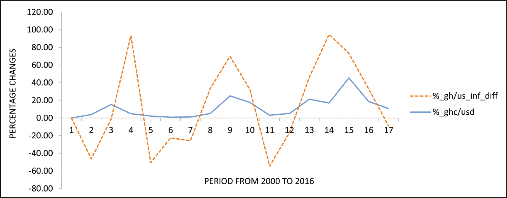
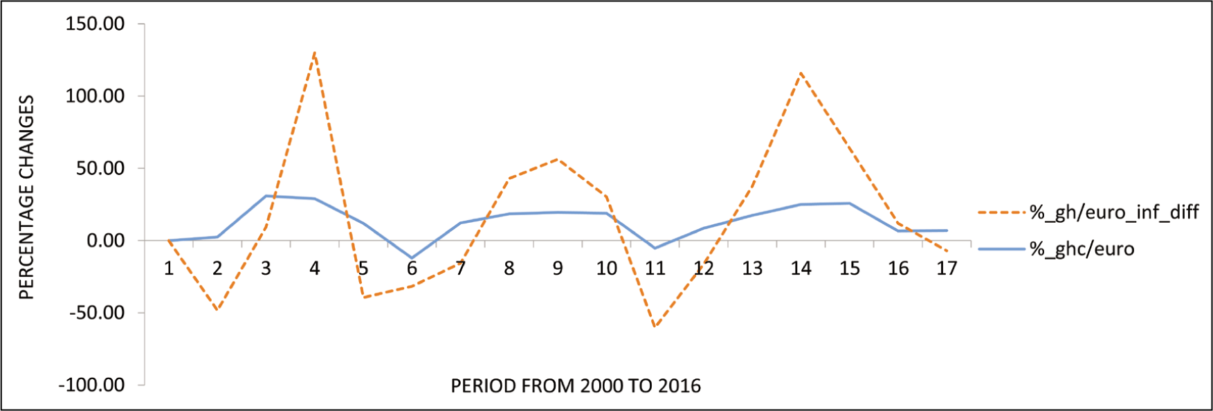
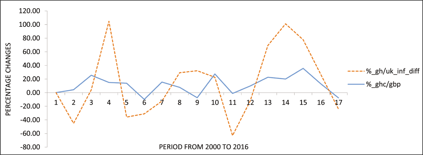
The interest rate rule operates on the basis of the Taylor principle which suggests a positive relationship between interest rates and inflation. The rule states that for every 1% increase in inflation, interest rates should be increased by more than 1%. The Taylor rule or principle is depicted in Figures 1–3. These figures show a positive general trend between the differential series. The Taylor rule is consistent with the International Fisher effect theory. This theory suggests that investors expect increase in interest rates when inflation increases as a compensation for the lost in value of their investment. The Fisher effect shares similarities with the Taylor rule, and was first formalized by Irwin Fisher (Hill, 2006). The Fisher effect considers high interest rates as a premium on inflationary risk. This is expressed as

Figure 1.

Cedi–Dollar Exchange Rate and Inflation Differential Plot.

Figure 2.

Cedi–Euro Exchange Rate and Inflation Differential Plot.

Figure 3.

Cedi–Pound Rate and Inflation Differential Plot.

I_{t} = {INF}_{t} + r_{t}

(3)

where I_t is the nominal interest rate, r_t is the real interest rate and INF_t is the inflation.

The Taylor rule is preliminary to the success of uncovered Interest rate parity (UIRP). The UIRP suggests that a currency with a higher interest rate is expected to depreciate by the amount of interest rate differential. This depreciation will make up for the gain in interest which will therefore prevent arbitrage profit in the foreign exchange market. The Taylor rule recommends a high nominal interest rate when inflation is above its target and output is above full employment. This is a case of monetary tightening. However, during periods of stagflation, where inflation is above its target and output is below full employment, the goals of monetary policy may conflict. The IMF Article IV Consultation Report (International Monetary Fund, 2017) recognizes this is the situation seldom experienced in Ghana. The remedy specified under the Taylor rule in this circumstance is to specify some relative weights for reducing inflation and some for increasing output. The IMF under the same report has also noted Ghana’s increasing desire to populate domestic output instead of bring inflation within target (Bhattarai & Armah, 2005; International Monetary Fund, 2017).

The interest rate parity is stated formally as the change in the spot exchange rate between two currencies A and B. This is expressed as

[\frac{(S_{1} - S_{2})}{S_{2}}] \times 100 = I_{A} - I_{B}

(4)

where S₁ is the spot rate at the beginning of the period, S₂ is the spot rate at the end of the period.

Balance of Payment Model

This model assumes exchange rate to be caused by tradable goods and services. It ignores the role of global capital flows in exchange rate determination. Exchange rate appreciations are linked to current account surplus and transactions in the model.

Asset Prices Model

This model views currencies as an important class of building investment portfolios. Asset prices or exchange rates are influenced mostly by peoples’ willingness to hold the existing quantities of assets or currencies which in turn depends on their expectations of the future worth of these assets. This model states that the exchange rate between two currencies represents the price that just balances the relative supplies of and demand for assets denominated in those currencies.

Empirical Review of Literature

Modelling and predicting Ghana’s exchange rate movements will need a decision to be made on model specifications. Work on exchange rate models, especially in an open economy, has evolved from specifying and comparing the forecast evaluation measures of models to now testing and comparing the significance of forecast evaluation measures. The empirical works of Rossi (2013), Carriero et al. (2009) and Cheung et al. (2005) have specified and compared the mean square forecast errors of fundamentally based econometric models such as the univariate models, error correction models, multivariate models and panel models with the mean square errors of random-walk models. These works have found the fundamentally based models to be statistically superior to the random-walk models. However, the conclusion reached by these researches is in sharp contrast with the view held in Abbate and Marcellino (2014), who believe most empirical studies support the superiority of the random walk models over the fundamentally based models. These differences in empirical works have led Takizawa et al. (2011) to assert that it is challenging to anticipate a likely winner between these competing exchange rate models and therefore different methodologies have produced mixed results and outcomes.

Petruccelli and Davies (1986), Yao and Rahaman (2018) and Hansen (1999, 2011) mentioned the significance of forecasting with non-linear models in another related development. They assert that non-linear models, as against linear models, can capture the dynamics and time irreversibility of a time series better than linear models. Additionally, it is also a well-known fact that the Gaussian linear time series models have failed to capture many phenomena commonly observed in practice (Tsay, 1991). This has led many researchers to propose non-linear specification of exchange rate modelling and that the non-linear models consistently outperform their linear counterparts in many respects (Ben Aïssa et al., 2004; Granger & Andersen, 1978; Maravall, 1983; Tong, 1983). For instance, in terms of forecasting accuracy and reliability, Tsay (1991) asserts that the non-linear models have moved time series analysis a step closer to reality. However, despite what has appeared to be a consensus of the non-linear models’ superiority, there is also general recognition of their difficulties and sophistication. We review a few of the literature on the difficulties in specifying a non-linear model and the methodologies in detecting non-linearity in time series data.

Many studies have shown that the BDS test, developed by Brock et al. (1987), has power against several ranges of linear and non-linear phenomena. The BDS test was developed to test the null of independent and identical distribution (IID) in time series and help detect non-random and chaotic dynamics. The strength of the BDS test is its ability to test for both non-linearity and model misspecification, which are the two main issues challenging non-linear analyses. Also, another equally relevant approach for testing non-linearity in a time series is the Tsay F-test statistic. The Tsay F-test approach or statistic detects a wide range of non-linear phenomena in time series data. For instance, the Tsay test is good in detecting bi-linearity. It can also detect threshold non-linearity and exponential non-linearity in a time series (Tsay, 1991). However, this test has a slight shortcoming in its approach to determining threshold non-linearity. The disadvantage of using the Tsay test (1986), including the test proposed by Petruccelli and Davies (1986), is the use of arranged autoregressive model in determining the thresholds that generally require knowledge of the threshold variable. Tsay (1989) asserts that the arranged autoregression only becomes useful for the threshold models when arranged according to the threshold variable. Our experience of the literature on threshold regression reveals that this threshold variable is primarily unknown by researchers. This, therefore, complicates Tsay’s approach in detecting threshold non-linearity, but it is still an essential tool in detecting non-linearity and widely used by researchers. Finally, an alternative test to the Tsay’s test and the Petruccelli and Davies approach is the Bai–Perron test. This test is equally good in detecting thresholds in times series and does not determine thresholds based on an arranged regression. This test is, therefore, functional even if the threshold variable is unknown. The procedure is based on multiply structural changes and allows one to test the null hypothesis of say i changes versus the alternative hypothesis of i + 1 changes. This is useful because it allows a specific-to-general modelling strategy to consistently determine the appropriate number of changes (Bai & Perron, 1998).

Research Methodology and Empirical Testing

Research Variables and Data

Molodtsova and Papell (2012) find that the predictions of Taylor rule models can be improved when supported with credit spread or measures of financial conditions. Sarno et al. (2004) also show evidence of the relationship between exchange rates and monetary fundamentals, and Lossifov and Loukoianova (2007) proved the prices of main export commodities also have an impact on Ghana’s exchange rate. Also, a report from the Bank of Ghana (May 2017) asserts that to reduce the cedi exchange rates’ volatilities, Ghana’s government has sought to reduce its external exposure by changing its debt structure to include more domestic debts. For these reasons, the research variable used in this research are carefully selected to include: exchange rates, gross reserves, broad money, short-term debts, and foreign direct investments.

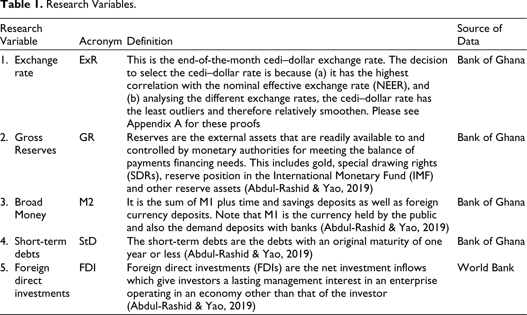
The data for the research is a monthly time series data taken from the Central Bank of Ghana’s database and from the World Bank database from the years 2000 to 2018. Table 1 shows the research variables and the sources from which data were taken.

Table 1.

Research Variables.

Research Variable	Acronym	Definition	Source of Data
1. Exchange rate	ExR	This is the end-of-the-month cedi–dollar exchange rate. The decision to select the cedi–dollar rate is because (a) it has the highest correlation with the nominal effective exchange rate (NEER), and (b) analysing the different exchange rates, the cedi–dollar rate has the least outliers and therefore relatively smoothen. Please see Appendix A for these proofs	Bank of Ghana
2. Gross Reserves	GR	Reserves are the external assets that are readily available to and controlled by monetary authorities for meeting the balance of payments financing needs. This includes gold, special drawing rights (SDRs), reserve position in the International Monetary Fund (IMF) and other reserve assets (Abdul-Rashid & Yao, 2019)	Bank of Ghana
3. Broad Money	M2	It is the sum of M1 plus time and savings deposits as well as foreign currency deposits. Note that M1 is the currency held by the public and also the demand deposits with banks (Abdul-Rashid & Yao, 2019)	Bank of Ghana
4. Short-term debts	StD	The short-term debts are the debts with an original maturity of one year or less (Abdul-Rashid & Yao, 2019)	Bank of Ghana
5. Foreign direct investments	FDI	Foreign direct investments (FDIs) are the net investment inflows which give investors a lasting management interest in an enterprise operating in an economy other than that of the investor (Abdul-Rashid & Yao, 2019)	World Bank

Specification of Linear Models and Test Outputs

Preliminary Testing

The variables were tested for stationarity or unit root. Tables 2 and 3 show the results of the unit root test. The test shows all the variables as stationary [I(0)]. Also, we found the variables gross reserves, broad money and short-term debts to have significant constant terms. We also found broad money to have a significant trend. We, therefore, specify and estimate the linear models with these deterministic features.

Table 2.

Unit Root Test (Analysis of Variables in First Difference).

Dependent Variable	Constant αˆ		Coefficient of Lag Regressors βˆ		Coefficients @ Trend		Augmented Dickey–Fuller Test H₀: Series Has a Unit Root H_A: Series Has No Unit Root
Dependent Variable	t-Statistic	Prob.	t-Statistic	Prob.	t-Statistic	Prob.	t-Statistic	5% Critical Value	Prob.
GR	2.6447	.0088^***	−17.0042	.0000^***	−1.5927	.1127	−17.0042	−3.4313	.0000^***
M2	8.8926	.0000^***	−10.5806	.0000^***	−2.8809	.0044^***	−10.5806	−3.4322	.0000^***
StD	2.1581	.0321^**	−16.8340	.0000^***	−0.7146	.4756	−16.8340	−3.4313	.0000^***
FDI	1.4185	.1575	−15.6848	.0000^***	−0.3439	.7312	−15.6848	−3.4313	.0000^***
ExR	0.7384	.4611	−5.5127	.0000^***	0.6797	.4975	−5.5127	−3.4315	.0000^***

Source: Bai and Perron (2003).

Notes: Decision rule on unit root testing: reject the null hypothesis when p value is less than or equal to .05 (5%) significance level or | t_s | > | t_T |. MaxLag = 12.

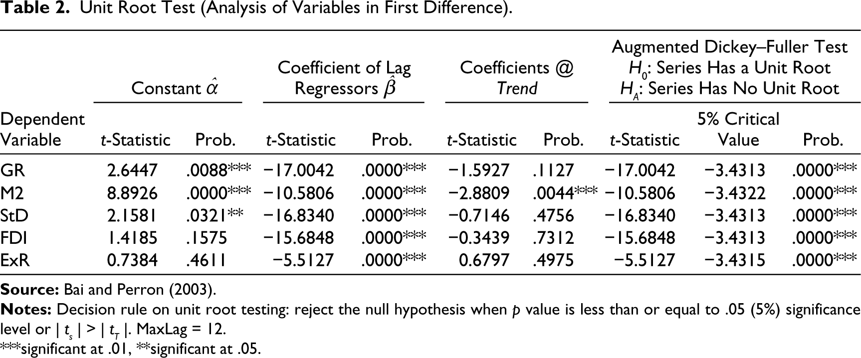
^***significant at .01, ^**significant at .05.

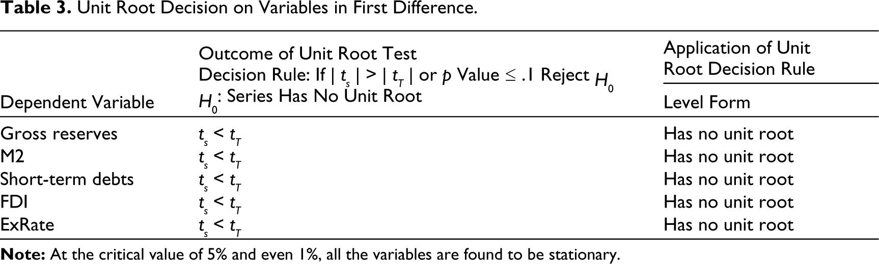
Also, a co-integration test was performed on the first difference of the variables, and the test revealed no co-integration existed in the transform state of the variables. Therefore, this output is withheld.

Table 3.

Unit Root Decision on Variables in First Difference.

Dependent Variable	Outcome of Unit Root Test Decision Rule: If \| t_s \| > \| t_T \| or p Value ≤ .1 Reject H₀ H₀: Series Has No Unit Root	Application of Unit Root Decision Rule
Dependent Variable		Level Form
Gross reserves	t_s < t_T	Has no unit root
M2	t_s < t_T	Has no unit root
Short-term debts	t_s < t_T	Has no unit root
FDI	t_s < t_T	Has no unit root
ExRate	t_s < t_T	Has no unit root

Note: At the critical value of 5% and even 1%, all the variables are found to be stationary.

Specifying Linear Models (i.e. a VAR Model and an ARIMA Model)

First, we specify a VAR model. Note that because there is no long-term relationship among the variables, we do not add an error term to the model. Therefore, we only specify a VAR(p) model, and impute into the model both trend and constant terms. These variables are added to the model because of the significant constant and trend in the unit root test table. In the final estimate of the VAR(p) model, we introduce a lagged exogenous variable into the model which is petroleum prices. This approach is to capture the research finding of Lossifov and Loukoianova (2007) that prices of main export or import commodities also have an impact on Ghana’s exchange rate.

The general VAR(p) model is therefore expressed as

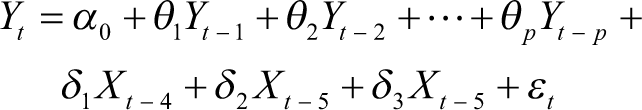
\begin{array}{l} Y_{t} = α_{0} + θ_{1} Y_{t - 1} + θ_{2} Y_{t - 2} + \dots + θ_{p} Y_{t - p} + \\ δ_{1} X_{t - 4} + δ_{2} X_{t - 5} + δ_{3} X_{t - 5} + ε_{t} \end{array}

(5)

where Y_t is a (k × 1) vector of endogenous variables; X is a (k × 1) vector of exogenous variables, that is, change in petroleum prices; α₀ is a (k × 1) vector of constant terms; θ_i is a (k × k) matrix of coefficients; δ_i is a matrix of exogenous coefficients; ε_t (k × 1) vector of error terms.

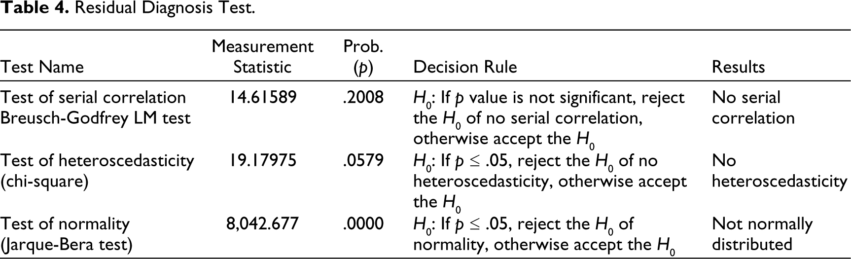
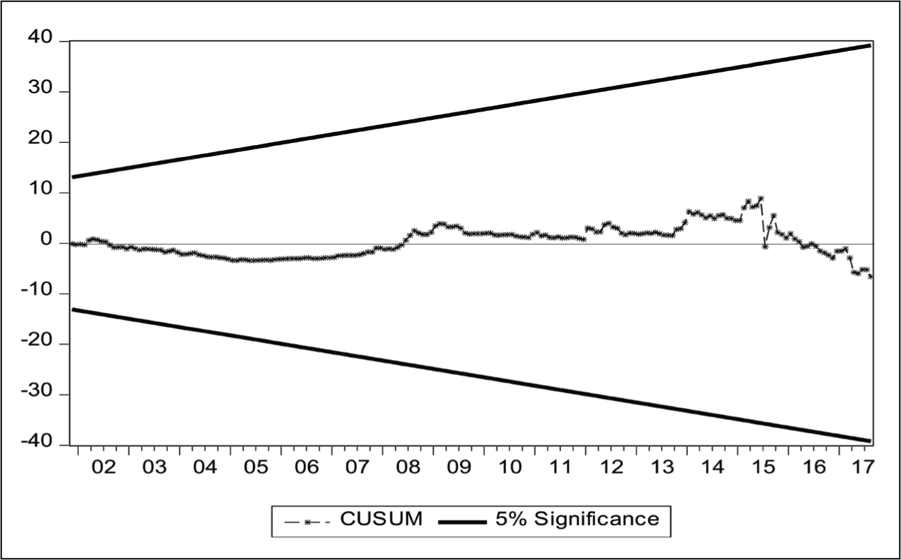
The model was tested for serial correlation, heteroscedasticity and normal distribution. Table 4 shows these residual diagnosis tests, and Figure 4 shows the parameter stability test of the model.

Table 4.

Residual Diagnosis Test.

Test Name	Measurement Statistic	Prob. (p)	Decision Rule	Results
Test of serial correlation Breusch-Godfrey LM test	14.61589	.2008	H₀: If p value is not significant, reject the H₀ of no serial correlation, otherwise accept the H₀	No serial correlation
Test of heteroscedasticity (chi-square)	19.17975	.0579	H₀: If p ≤ .05, reject the H₀ of no heteroscedasticity, otherwise accept the H₀	No heteroscedasticity
Test of normality (Jarque-Bera test)	8,042.677	.0000	H₀: If p ≤ .05, reject the H₀ of normality, otherwise accept the H₀	Not normally distributed

Figure 4.

Parameter Stability Test.

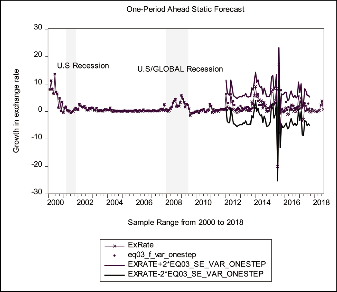
The forecast measures of the VAR model are summarized in Table 5. The root mean square error (RMSE) and the Theil inequality coefficient are lesser for the one-period ahead forecast than the multiple-period ahead forecasts. This result means the prediction for the one-period ahead forecast is more accurate for the VAR model than the prediction of the multiple-period ahead forecast. Figures 5 and 6 show the forecast graphs of the VAR model.

Table 5.

Forecast Performance Evaluation Measures of the VAR(11) Model.

Model	Forecast Horizon
Model	One-period Ahead Static Forecast	Multiple-period Ahead Static Forecast
Root mean square error	3.8757	0.9688
Theil inequality coefficient	0.5676	0.7453
Bias proportion	0.0019	0.0000
Variance proportion	0.3983	0.5750
Covariance proportion	0.5996	0.4249

Figure 5.

One-period Ahead Forecast Graph_VAR Model.

Figure 6.

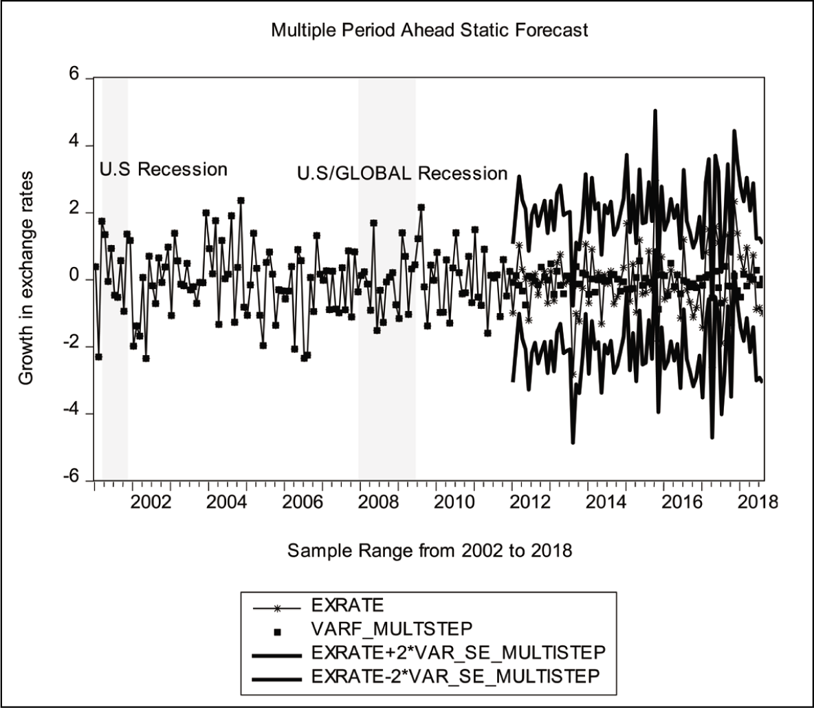
Multiple-period Ahead Forecast Graph_VAR Model.

ARIMA Model

Second, we specify an autoregressive integrated moving average (ARIMA) model by following the BJ (Box–Jenkins) methodology. In the BJ methodology, the first approach is to identify the appropriate values of the autoregressive lags (p), the number of times the series is differentiated (d), and the number of moving average terms (q).

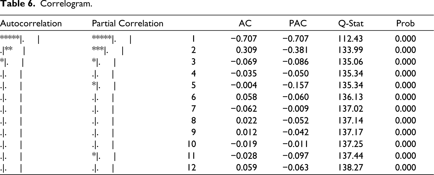
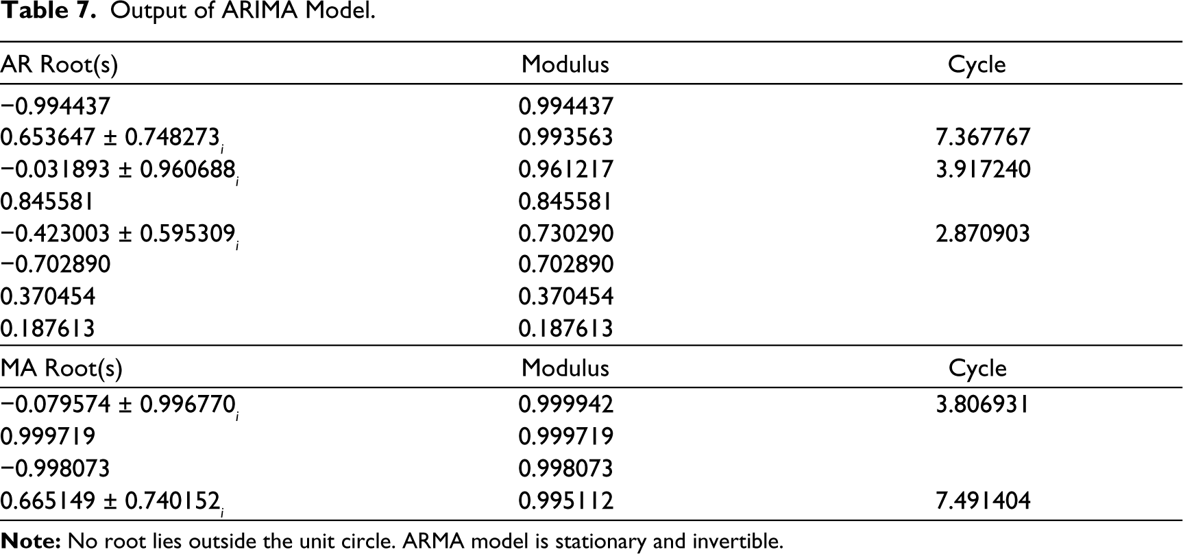
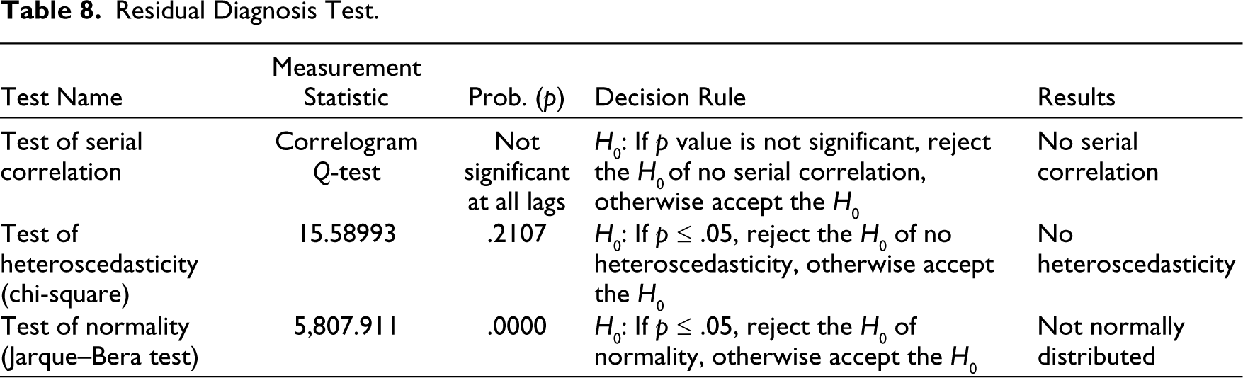
For the order of integration (d), we have shown in the VAR model that the cedi–dollar exchange rate is an integration of order 1, that is, [I(1)]. Table 6 shows the correlogram which will enable us to determine the values of p and q. From the correlogram, we observed that the PACF is significant up to the 11th lag and the ACF has only two significant lags. The outlook of the table gives an ARIMA (11, 1, 2); however, the final fitted model is an ARIMA (11, 1, 6). The estimated output of this model is presented in Table 7. Also, the residual diagnosis test of this model is shown in Table 8.

Table 6.

Correlogram.

Autocorrelation	Partial Correlation		AC	PAC	Q-Stat	Prob
^*****\|. \|	^*****\|. \|	1	−0.707	−0.707	112.43	0.000
.\|^** \|	^***\|. \|	2	0.309	−0.381	133.99	0.000
^*\|. \|	^*\|. \|	3	−0.069	−0.086	135.06	0.000
.\|. \|	.\|. \|	4	−0.035	−0.050	135.34	0.000
.\|. \|	^*\|. \|	5	−0.004	−0.157	135.34	0.000
.\|. \|	.\|. \|	6	0.058	−0.060	136.13	0.000
.\|. \|	.\|. \|	7	−0.062	−0.009	137.02	0.000
.\|. \|	.\|. \|	8	0.022	−0.052	137.14	0.000
.\|. \|	.\|. \|	9	0.012	−0.042	137.17	0.000
.\|. \|	.\|. \|	10	−0.019	−0.011	137.25	0.000
.\|. \|	^*\|. \|	11	−0.028	−0.097	137.44	0.000
.\|. \|	.\|. \|	12	0.059	−0.063	138.27	0.000

Table 7.

Output of ARIMA Model.

AR Root(s)	Modulus	Cycle
−0.994437	0.994437
0.653647 ± 0.748273_i	0.993563	7.367767
−0.031893 ± 0.960688_i	0.961217	3.917240
0.845581	0.845581
−0.423003 ± 0.595309_i	0.730290	2.870903
−0.702890	0.702890
0.370454	0.370454
0.187613	0.187613
MA Root(s)	Modulus	Cycle
−0.079574 ± 0.996770_i	0.999942	3.806931
0.999719	0.999719
−0.998073	0.998073
0.665149 ± 0.740152_i	0.995112	7.491404

Note: No root lies outside the unit circle. ARMA model is stationary and invertible.

Table 8.

Residual Diagnosis Test.

Test Name	Measurement Statistic	Prob. (p)	Decision Rule	Results
Test of serial correlation	Correlogram Q-test	Not significant at all lags	H₀: If p value is not significant, reject the H₀ of no serial correlation, otherwise accept the H₀	No serial correlation
Test of heteroscedasticity (chi-square)	15.58993	.2107	H₀: If p ≤ .05, reject the H₀ of no heteroscedasticity, otherwise accept the H₀	No heteroscedasticity
Test of normality (Jarque–Bera test)	5,807.911	.0000	H₀: If p ≤ .05, reject the H₀ of normality, otherwise accept the H₀	Not normally distributed

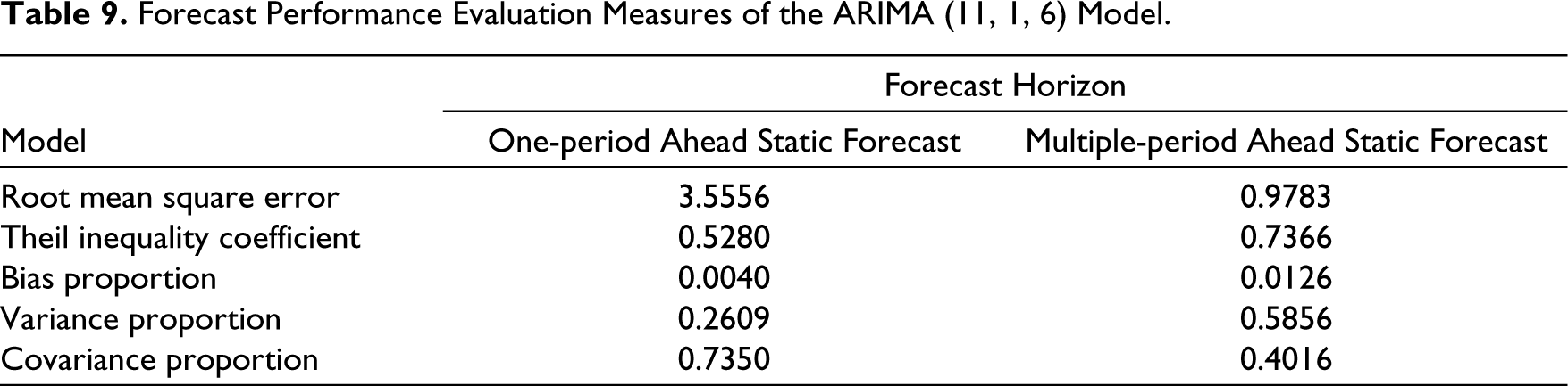
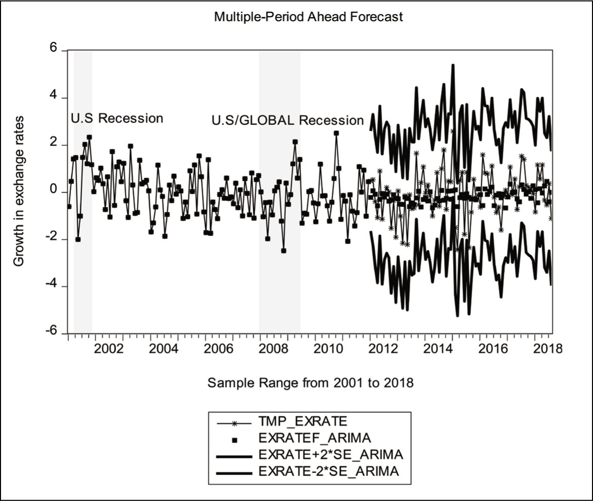
The forecast measures of the ARIMA (11, 1, 6) is that the RMSE and the Theil inequality coefficient are lesser for the one-period ahead forecast than the multiple-period ahead forecasts. This is shown in Table 9. The result, again, shows that the one-period ahead forecast prediction of the ARIMA model is more accurate and closer to the actual values than the multiple-period ahead forecast prediction. Figures 7 and 8 show the forecast graphs of the ARIMA model.

Table 9.

Forecast Performance Evaluation Measures of the ARIMA (11, 1, 6) Model.

Model	Forecast Horizon
Model	One-period Ahead Static Forecast	Multiple-period Ahead Static Forecast
Root mean square error	3.5556	0.9783
Theil inequality coefficient	0.5280	0.7366
Bias proportion	0.0040	0.0126
Variance proportion	0.2609	0.5856
Covariance proportion	0.7350	0.4016

Figure 7.

One-period Ahead Forecast Graph.

Figure 8.

Multiple-period Ahead Forecast Graph.

Specification of a Non-linear Model and Test Output

Before we proceed with estimating a non-linear model, we need to establish that (a) the cedi–dollar exchange rate is non-linear and (b) which type of non-linear series is the cedi–dollar exchange rate?

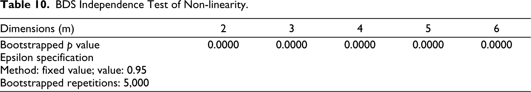
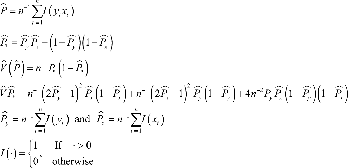
To address these issues, we employed the Brock, Dechert and Scheinkman (BDS) independence test and the Bai–Perron test statistics, respectively. Tables 10 and 11 show the test output of the BDS test and Bai–Perron test statistics, respectively. The BDS test output shows the cedi–dollar rate series is non-linear, and therefore, predictions of the series values are better captured by a non-linear model. Also, the Bai–Perron test results show the presence of thresholds in the cedi–dollar rates and therefore specifying a self-exciting threshold autoregression (SETAR) model fits the data correctly (Gibson & Nur, 2011; Gyamfi & Kyei, 2016; Haggan et al., 1984; Lossifov & Loukoianova, 2007). The SETAR model is specified below:

Table 10.

BDS Independence Test of Non-linearity.

Dimensions (m)	2	3	4	5	6
Bootstrapped p value Epsilon specification Method: fixed value; value: 0.95 Bootstrapped repetitions: 5,000	0.0000	0.0000	0.0000	0.0000	0.0000

Table 11.

Bai–Perron Test of L + 1 Versus L Sequentially Determined Thresholds.

Sequential F-Statistic Determined Thresholds			4
Threshold Test	F-Statistic	Scaled F-Statistic	Critical Value^**
0 vs. 1^*	12.09051	145.0862	27.03
1 vs. 2^*	8.098594	97.18313	29.24
2 vs. 3^*	3.038271	36.45926	30.45
3 vs. 4^*	3.957152	47.48582	31.45
4 vs. 5	1.803918	21.64702	32.12

*Significant at the 0.05 level; **Bai–Perron (Bai & Perron, 2003) critical values.

A time-series data is said to follow a j-regime self-exciting threshold autoregressive (SETAR) model with a threshold variable Z_t_{– 1} if it satisfies:

Y_{t} = μ + \sum_{i = 1}^{p} θ_{i} X_{t - 1}^{(j)} + ε_{t}, if Γ_{j - 1} < Z_{t - d} \leq Γ_{j}

(6)

where θ is the autoregressive parameters; σ is the standard noise deviation; Γ is the threshold parameter; ε is a sequence of IID random variables with mean 0 and variance 1.

The general form of the SETAR model is

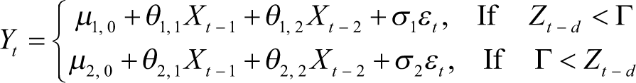
Y_{t} = {\begin{matrix} μ_{1, 0} + θ_{1, 1} X_{t - 1} + θ_{1, 2} X_{t - 2} + σ_{1} ε_{t}, If Z_{t - d} < Γ \\ μ_{2, 0} + θ_{2, 1} X_{t - 1} + θ_{2, 2} X_{t - 2} + σ_{2} ε_{t}, If Γ < Z_{t - d} \end{matrix}

From the general model, the parameters are in the lower regime if the threshold variable (Z_t_{– d}) is lower than the threshold value (Γ) and in the upper regime, if the threshold variable (Z_t_{– d}) is greater than the threshold value (Γ). This process is the regime-switching process between linear models and is dependent on the position of the threshold variable (Z_t_{– d}). Our fitted SETAR (5, 11) model is therefore:

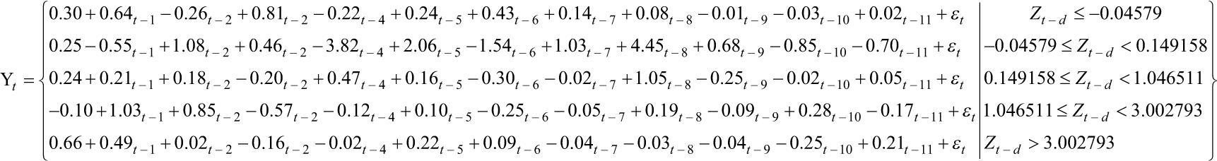
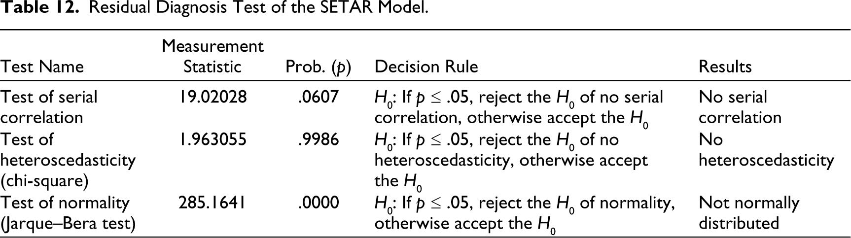
Y_{t} = {\begin{array}{l} 0.30 + {0.64}_{t - 1} - {0.26}_{t - 2} + {0.81}_{t - 2} - {0.22}_{t - 4} + {0.24}_{t - 5} + {0.43}_{t - 6} + {0.14}_{t - 7} + {0.08}_{t - 8} - {0.01}_{t - 9} - {0.03}_{t - 10} + {0.02}_{t - 11} + ε_{t} \\ 0.25 - {0.55}_{t - 1} + {1.08}_{t - 2} + {0.46}_{t - 2} - {3.82}_{t - 4} + {2.06}_{t - 5} - {1.54}_{t - 6} + {1.03}_{t - 7} + {4.45}_{t - 8} + {0.68}_{t - 9} - {0.85}_{t - 10} - {0.70}_{t - 11} + ε_{t} \\ 0.24 + {0.21}_{t - 1} + {0.18}_{t - 2} - {0.20}_{t - 2} + {0.47}_{t - 4} + {0.16}_{t - 5} - {0.30}_{t - 6} - {0.02}_{t - 7} + {1.05}_{t - 8} - {0.25}_{t - 9} - {0.02}_{t - 10} + {0.05}_{t - 11} + ε_{t} \\ - 0.10 + {1.03}_{t - 1} + {0.85}_{t - 2} - {0.57}_{t - 2} - {0.12}_{t - 4} + {0.10}_{t - 5} - {0.25}_{t - 6} - {0.05}_{t - 7} + {0.19}_{t - 8} - {0.09}_{t - 9} + {0.28}_{t - 10} - {0.17}_{t - 11} + ε_{t} \\ 0.66 + {0.49}_{t - 1} + {0.02}_{t - 2} - {0.16}_{t - 2} - {0.02}_{t - 4} + {0.22}_{t - 5} + {0.09}_{t - 6} - {0.04}_{t - 7} - {0.03}_{t - 8} - {0.04}_{t - 9} - {0.25}_{t - 10} + {0.21}_{t - 11} + ε_{t} \end{array} | \begin{matrix} Z_{t - d} \leq - 0.04579 \\ \begin{array}{l} - 0.04579 \leq Z_{t - d} < 0.149158 \\ 0.149158 \leq Z_{t - d} < 1.046511 \\ 1.046511 \leq Z_{t - d} < 3.002793 \\ Z_{t - d} > 3.002793 \end{array} \end{matrix}}

Table 12 shows the residual diagnosis of the SETAR model. The Jarque–Bera test statistic indicates the residuals of the series are not normally distributed, but this condition can be improved with data additions.

Table 12.

Residual Diagnosis Test of the SETAR Model.

Test Name	Measurement Statistic	Prob. (p)	Decision Rule	Results
Test of serial correlation	19.02028	.0607	H₀: If p ≤ .05, reject the H₀ of no serial correlation, otherwise accept the H₀	No serial correlation
Test of heteroscedasticity (chi-square)	1.963055	.9986	H₀: If p ≤ .05, reject the H₀ of no heteroscedasticity, otherwise accept the H₀	No heteroscedasticity
Test of normality (Jarque–Bera test)	285.1641	.0000	H₀: If p ≤ .05, reject the H₀ of normality, otherwise accept the H₀	Not normally distributed

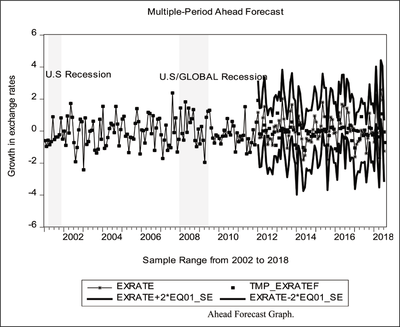
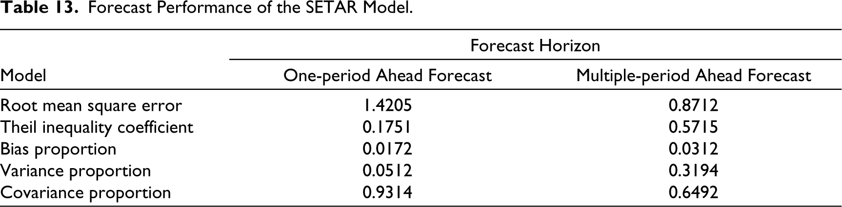
Figures 9 and 10 show a one-period ahead forecast and a multiple-period ahead forecast of the SETAR (5, 11) model. These figures marked the United States’ low economic periods, that is, the recession of 2001 and the global financial crisis from late 2007 to early 2009. The plot of the actual rates (represented by an asterisk line x) and the forecasted rates (represented by a square box) from 2011 to 2018 shows a relatively narrow gap than the plots in Figure 10 (the multiple-period ahead forecast). This narrowing gap shows that the forecasts produced in Figure 9 are superior and better than the forecasts in Figure 10. The results in Table 13 confirm the observations from the figures. Table 13 shows the forecast evaluation measures of the SETAR non-linear model. The RMSE of the SETAR model is lesser for the multiple-period ahead forecast. This lesser value of 0.8712 means the predicted values of the non-linear model for the multiple-period ahead forecast are superior to a one-period ahead forecast. The other measurements, that is, the Theil inequality, the Bias proportion, variance proportion and the covariance proportions, are sub-measures or components of the RMSE. We will discuss these sub-measures in the ‘Results and Discussions’ section.

Figure 9.

One-period Ahead Forecast Graph.

Figure 10.

Multiple-period Ahead Forecast Graph.

Table 13.

Forecast Performance of the SETAR Model.

Model	Forecast Horizon
Model	One-period Ahead Forecast	Multiple-period Ahead Forecast
Root mean square error	1.4205	0.8712
Theil inequality coefficient	0.1751	0.5715
Bias proportion	0.0172	0.0312
Variance proportion	0.0512	0.3194
Covariance proportion	0.9314	0.6492

Comparison between the Forecast Evaluation Measures

The forecast evaluation measures of the competing models are compared using both the traditional forecast evaluation measures and the advanced forecast evaluation measures.

Traditional Forecast Evaluation Measures

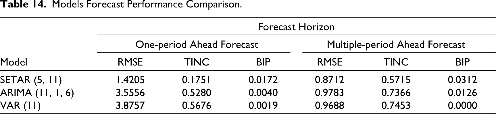
According to the RMSEs and the Theil inequality coefficients, forecasting with the non-linear SETAR model returns better predictions of the actual values in both the single-period ahead forecasts and the multiple-period ahead forecasts, while the ARIMA model produces better superior predictions among the linear models over a shorter horizon. These statistics are shown in Table 14.

Table 14.

Models Forecast Performance Comparison.

Model	Forecast Horizon
	One-period Ahead Forecast			Multiple-period Ahead Forecast
	RMSE	TINC	BIP	RMSE	TINC	BIP
SETAR (5, 11)	1.4205	0.1751	0.0172	0.8712	0.5715	0.0312
ARIMA (11, 1, 6)	3.5556	0.5280	0.0040	0.9783	0.7366	0.0126
VAR (11)	3.8757	0.5676	0.0019	0.9688	0.7453	0.0000

Advanced Forecast Evaluation Measures

Having analysed the linear and non-linear models’ forecast measures using the traditional methods, we go a step further by determining whether this difference is significant or simply due to specification error. In this research, we used the DM test statistic to check the comparison made between the forecasts of the linear and non-linear models. We also used the PT test to determine whether the models’ forecasts are accurate in predicting changes in the direction of the exchange rates. According to Ince and Molodtsova (2017), Haggan et al. (1984) and Aïssa and Jouini (2003), the latter approach is vital because of hyper-inflation, high-interest rates, political instability and growing external exposures which often cause a sudden change in the direction of the exchange rates in developing countries. Also, for market participants whose sole aim is to maximize gains and reduce losses in the foreign exchange market, knowing the direction of the change is significant to decide whether to buy (take a long position) or sell (take a short position) in the market.

The DM test makes use of the differential loss function (d) of two forecasts residuals, that is, e_1t and e_2t. The DM test is

d_{t} = g (e_{1 t}) - g (e_{2 t})

(7)

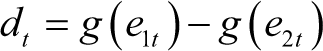
where 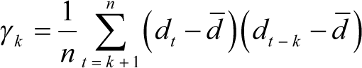$\bar{d} = (1 / n) \sum_{t = 1}^{n} d_{t}$ and μ = E(d_t). For n > k ≥ 1, defined as

γ_{k} = \frac{1}{n} \sum_{t = k + 1}^{n} (d_{t} - \bar{d}) (d_{t - k} - \bar{d})

For h ≥ 1, define the Diebold–Mariano statistic as follows:

DM = \frac{\bar{d}}{\sqrt{[γ_{0} + 2 \sum_{k = 1}^{h - 1} γ_{k}] / n}}

(8)

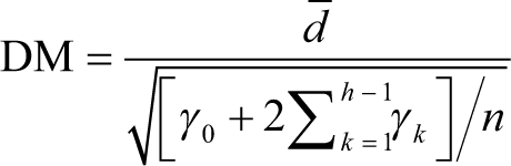
The hypotheses test of the Diebold–Mariano test statistics is H₀: E(d_t) = 0, that is, the two forecasts have the same accuracy; H₁: E(d_t) ≠ 0, that is, the two forecasts have different levels of accuracy.

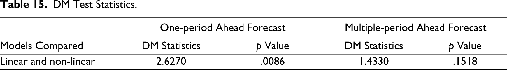
Table 15 and Figures 11 and 12 show the linear and non-linear models’ DM test statistics in both one-step and multiple-step forecast horizons. Note here that the VAR model represents the linear model because it has a better prediction than the ARIMA model. Therefore, the actual comparison of the models is between the VAR model and the SETAR model. The DM test statistics return a significant p value in the one-period ahead forecast horizon, implying that the differences between the models are significant and merit attention in a one-period ahead forecast horizon. For the directional forecasting accuracy, Pesaran and Timmermann (1992) used a non-parametric test to examine the effectiveness of a forecast to predict the direction of a change in a series of interest. This approach computes the proportion of the forecast values with the same sign as the actual series data. Assume we denote the series of interest as y_t and its forecasts are x_t, the PT test is defined as

S_{n} = \frac{\hat{p} - \hat{p_{*}}}{{[\hat{V} (\hat{P}) - \hat{V} (\hat{P_{*}})]}^{0.5}}

(9)

Table 15.

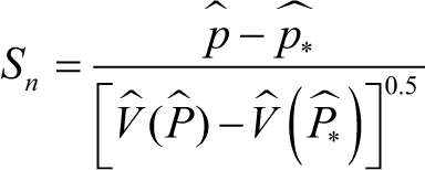
DM Test Statistics.

Models Compared	One-period Ahead Forecast		Multiple-period Ahead Forecast
Models Compared	DM Statistics	p Value	DM Statistics	p Value
Linear and non-linear	2.6270	.0086	1.4330	.1518

Figure 11.

DM Test Statistic One-step Ahead Forecast Graph of the Linear and Non-linear Model.

Figure 12.

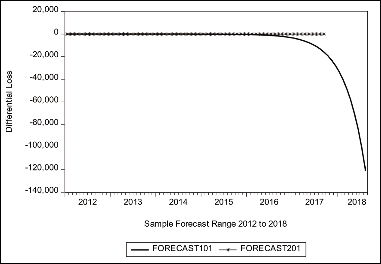
DM Test Statistic Multiple-period Ahead Forecast Graph of the Linear and Non-linear Models.

where

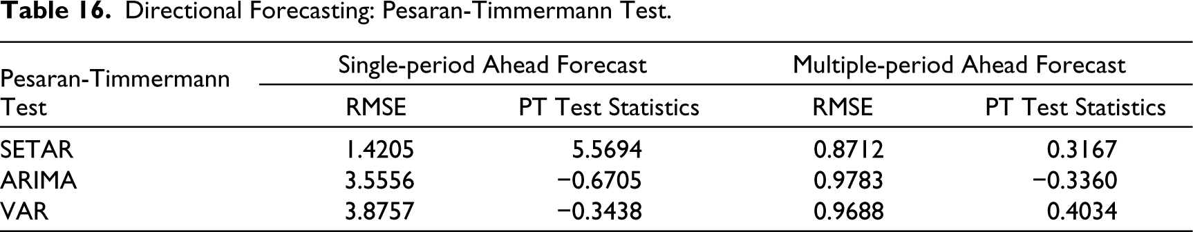
\begin{array}{l} \hat{P} = n^{- 1} {\sum^{​}}^{​}_{t = 1}^{n} I (y_{t} x_{t}) \\ \hat{P_{*}} = \hat{P_{y}} \hat{P_{x}} + (1 - \hat{P_{y}}) (1 - \hat{P_{x}}) \\ \hat{V} (\hat{P}) = n^{- 1} P_{*} (1 - \hat{P_{*}}) \\ \hat{V} \hat{P_{*}} = n^{- 1} (^{2 \hat{P_{y}} - 1) 2} \hat{P_{x}} (1 - \hat{P_{x}}) + n^{- 1} (^{2 \hat{P_{x}} - 1) 2} \hat{P_{y}} (1 - \hat{P_{y}}) + 4 n^{- 2} P_{y} \hat{P_{x}} (1 - \hat{P_{y}}) (1 - \hat{P_{x}}) \\ \hat{P_{y}} = n^{- 1} {\sum^{​}}^{​}_{t = 1}^{n} I (y_{t}) a n d \hat{P_{x}} = n^{- 1} {\sum^{​}}^{​}_{t = 1}^{n} I (x_{t}) \\ I (\cdot) = {\begin{matrix} 1 \\ 0 \end{matrix}, \begin{matrix} I f \cdot > 0 \\ o t h e r w i s e \end{matrix} \end{array}

Under the null hypothesis of x_t not been able to predict y_t. Note that S_n also follows the standard normal distribution. Table 16 shows the PT test statistics for the various models.

Table 16.

Directional Forecasting: Pesaran-Timmermann Test.

Pesaran-Timmermann Test	Single-period Ahead Forecast		Multiple-period Ahead Forecast
Pesaran-Timmermann Test	RMSE	PT Test Statistics	RMSE	PT Test Statistics
SETAR	1.4205	5.5694	0.8712	0.3167
ARIMA	3.5556	−0.6705	0.9783	−0.3360
VAR	3.8757	−0.3438	0.9688	0.4034

Results and Discussions

The models’ forecast evaluation measures return lower comparative RMSE and Theil inequality coefficient values for the non-linear SETAR model for both the one-period ahead forecast and the multiple-period ahead forecasts. These statistics imply that the non-linear SETAR model’s forecast values are closer and nearer to the actual exchange rate values than the comparable linear models. This finding confirms the findings in Granger and Andersen (1978), Maravall (1983), Tong (1983) and Tsay (1991). However, the comparison between the linear models, that is, the ARIMA and VAR model, reveals some slight advantage of the ARIMA model over the VAR model in a one-period ahead forecast, but the VAR model also has the advantage in a multi-period ahead forecast.

The research on comparing the forecast accuracy of econometric forecasting models has now gone beyond the mere comparison of forecast evaluation measures. Recent empirical works now move the comparison a little higher to comparing the statistical significance of these forecast evaluation measures. For this reason, we have computed the DM test statistics to improve the level of our comparison. The DM test statistics have found that the differences in the linear models’ forecast performance measures and the non-linear model is statistically significant. This result means that the predictions of the models are significantly different and merit attention by businesses in forecasting the cedi exchange rates in a one-period ahead forecast. However, the significance test was rejected in the multiple-period ahead forecasts, meaning the models do not perform differently in the long run.

For forecasting the directional movements of the cedi exchange rate, the PT test statistics have found that the non-linear SETAR model is superior for forecasting the exchange rate movements in one-period ahead forecasts. However, the VAR model produces a better prediction of the direction of change in the cedi exchange rate for a multiple-period ahead forecast despite it having a relatively higher mean square error than the non-linear model. This result confirms the assertion in Abbate and Marcellino (2014) that the linear models added with macroeconomic differentials have higher predictive likelihoods at long horizons and during periods of recession. Ince and Molodtsova (2017) and Engle and Hamilton (1990) highlight the relevance of testing the econometric models for directional accuracy, especially in developing nations characterized by high inflationary figures, high interest rates, political instability, and high external exposures, which often causes swift changes in the directional movement of the exchange rates. Also, for market agents who operate to profit from exchange rate movements, predicting the directional movement of the exchange rate is essential to reducing forex losses (Abdul-Rashid et al., 2022; Cook, 2014; Leitch & Tanner, 1991; Pesaran & Timmermann, 1992).

Conclusions

The SETAR model produces better forecasts in terms of relative magnitude and directional trends of the exchange rate in a one-period ahead forecast horizon. The SETAR model is also superior in multiple-period ahead horizon forecasts, but the precision is only in predicting the magnitude of the change (and not in predicting the direction of the change). For predicting the directional change in exchange rates, in multiple-period ahead horizon forecasts, the VAR model has a better precision of the volatilities in exchange rate. These conclusions have insight for business owners or businesses whose operations are affected by forex movements. For short-term business commitments or transactions such as raw material purchases, cash expenses or incomes, business owners should plan or predict exchange rate movements using the SETAR or a non-linear model. However, for long-term contractual obligations like futures and forward contracts, the VAR or a multivariate linear model should be used in planning the management of forex losses.

Also, businesses which are established to trade in the cedi forex market or on the larger capital market with cedi-denominated securities can benefit from these research conclusions to minimize losses in the capital market.

Bléjer et al. (2000), Lossifov and Loukoianova (2007), Salachas et al. (2017) and International Monetary Fund (2017) provide technical advice to independent policymakers to wrap up any process of successful implementation of monetary and fiscal policy framework by having reliable forecasts of target variables (in this case the exchange rates). This research, especially the aspect of the directional prediction of the exchange rate, will also help policymakers in adjusting the policy tools in efforts to stabilize the economy.

Recommendation for Future Research

Further research can consider a panel study of businesses in Ghana by analysing their financial statements and reporting the losses that these research conclusions could have helped save.

Footnotes

Declaration of Conflicting Interests

The authors declared no potential conflicts of interest with respect to the research, authorship and/or publication of this article.

Funding

The authors received no financial support for the research, authorship and/or publication of this article.

Appendix A. Choice of Research Variable

According to BoG (2018), the nominal effective exchange rate (NEER) provides a much more comprehensive assessment of the cedi than any exchange rate series of key trading partners. However, this research intends to use Ghana’s exchange rate with one of its key trading partners, but this rate should also be a good proxy to the NEER. This approach is to enable us benefit from the analysis with single exchange rate data whiles at the same time not losing the benefits of the composite effect in the NEER.

This research has therefore used three strategies to select the exchange rate that can be a good proxy to the NEER in the analysis.

First, the research analyses the correlations of each key partner’s exchange rates with the NEER in .

The cedi-dollar exchange rates were found to have the highest correlation with the NEER, and can be a good proxy to the NEER with this strategy adopted.

Secondly, the research looked at the strategy of outliers, and again choosing the right exchange rates with the least outliers. The box plot of the various exchange rates series is shown below:

The cedi-dollar rates series were again found to have the least outliers and was again chosen by this strategy as the right proxy for the nominal effective exchange rates.

Therefore, concluding on the two strategies, the research has selected the cedi-dollar rates as the best proxy for the NEER series.

References

Abbate

, & Marcellino

(2014). Modelling and forecasting exchange rates with time-varying parameter models. Journal of Economic Literature, 17(1–2), 233–261.

Abdul-Rahaman

A. R.

, & Yao

(2019). Reserves quantity and economic stability: The central bank of Ghana’s position and practices. Heliyon, 5(12), 28–56.

Abdul-Rashid

A. R.

, Yao

, Abdul-Rasheed

A. A.

, Emmanuel

C. A.

, Jean Baptiste Bernand

, & Mohammed Kamil

(2022). Optimal foreign exchange reserve: Protection against external shocks in Ghana. Frontiers in Psychology, 13, 994043. 10.3389/fpsyg.2022.994043

Abradu-Otoo

, Amoah

, & Bawumia

(2003). An investigation of the transmission mechanisms of monetary policy in Ghana: A structural vector error correction analysis. Working paper 2. Bank of Ghana.

Aïssa

M. S. B.

, and Jouini

(2003). Structural breaks in the US inflation process. Applied Economics Letters, 10(10), 633–636.

Bai

, & Perron

(1998). Estimating and testing linear models with multiple structural changes. Econometrica, 66(1), 47–78.

Bai

, & Perron

(2003). Critical values for multiple structural change tests. The Econometrics Journal, 6(1), 72–78.

Bank of Ghana Statistics and Reports Office. (2018). Brief history of the Ghana currency. Bank of Ghana Statistics and Reports Office. https://bog.gov.gh/index.php?option=com_content&view=article&id=105&Itemid=164

Ben Aïssa

M. S.

, Boutahar

, & Jouini

(2004). Bai and Perron’s and spectral density methods for structural change detection in the US inflation process. Applied Economics Letters, 11(2), 109–115.

10.

Bhattarai

, & Armah

M. K.

(2005). The effects of exchange rate on the trade balance in Ghana: Evidence from cointegration analysis. Business School, University of Hull.

11.

Bléjer

M. M. I.

, Ize

M. A.

, Leone

M. A. M.

, & da Costa Werlang

M. S. R.

(Eds.). (2000). Inflation targeting in practice: strategic and operational issues and application to emerging market economies. International Monetary Fund.

12.

Blinder

(1998). Central banking in theory and practice. MIT Press.

13.

BoG. (May 2017). Monetary policy report (vol. 2.1). Bank of Ghana.

14.

Brock

, Dechert

W. D.

, & Scheinkman

(1987). A test for independence based on the correlation dimension. Economics working paper SSRI-8702. University of Wisconsin.

15.

Cassel

(1918). Abnormal deviations in international exchanges. The Economic Journal, 28, 413–415.

16.

Cook

(2014). Directional forecasting, forecasting accuracy, and making profits. Economics Network. www.economicsnetwork.ac.uk/showcase/cook_directional

17.

Carriero

, Kapetanios

, & Marcellino

(2009). Forecasting exchange rates with a large Bayesian VAR. International Journal of Forecasting, 25(2), 400–417.

18.

Cheung

Y. W.

, Chinn

M. D.

, & Pascual

A. G.

(2005). Empirical exchange rate models of the nineties: Are any fit to survive? Journal of International Money and Finance, 24(7), 1150–1175.

19.

De Rosa

M. L.

, Schrijver

C. J.

, Barnes

, Leka

K. D.

, Lites

B. W.

, Aschwanden

M. J.

, Amari

, Canou

, McTiernan

, Régnier

, Thalmann

J. K.

, Valori

, Wheatland

, Wiegelmann

, Cheung

M. C. M.

, Conlon

P. A.

, Fuhrmann

, Inhester

, Tadesse

(2009). A critical assessment of nonlinear force-free field modeling of the solar corona for active region 10953. The Astrophysical Journal, 696(2), 1780–1791.

20.

Engle

, & Hamilton

J. D.

(1990). Long swings in the dollar: Are they in the data and do markets know it. American Economic Review, 80(4), 689–713.

21.

Granger

C. W. J.

, & Andersen

A. P.

(1978). An introduction to bilinear time series models. Vandenhoek and Ruprecht.

22.

Granger

C. W.

, & Pesaran

M. H.

(2000). Economic and statistical measures of forecast accuracy. Journal of Forecasting, 19(7), 537–560.

23.

Gibson

, & Nur

(2011). Threshold autoregressive models in finance: A comparative approach. In Proceedings of the fourth annual ASEARC conference. University of Western Sydney, Paramatta, Australia.

24.

Gyamfi

E. N.

, & Kyei

K. A.

(2016). Modeling stock market returns under self-exciting threshold autoregressive model: Evidence from West Africa. International Journal of Economics and Financial Issues, 6(3), 1194–1199.

25.

Haggan

, Heravi

S. M.

, & Priestley

M. B.

(1984). A study of the application of state-dependent models in non-linear time series analysis. Journal of Time Series Analysis, 5(2), 69–102.

26.

Hansen

B. E.

(1999). Testing for linearity. Journal of Economic Surveys, 13(5), 551–576.

27.

Hansen

B. E.

(2011). Threshold autoregression in economics. Statistics and Its Interface, 4(2), 123–127.

28.

Hauner

, Janni

, Rack

, & Hauner

(2011). The effect of overweight and nutrition on prognosis in breast cancer. Deutsches Ärzteblatt International, 108(47), 795.

29.

Hill

(2006). Ownership structure and IPO underpricing. Journal of Business Finance and Accounting, 33(1–2), 102–126. 10.1111/j.1468-5957.2006.01359.x

30.

Ince

, & Molodtsova

(2017). Rationality and forecasting accuracy of exchange rate expectations: Evidence from survey-based forecasts. Journal of International Financial Markets, Institutions, and Money, 47, 131–151. 10.1016/j.intfin.2016.11.002

31.

International Monetary Fund. (September 2017). IMF Article IV consultation report. Country report 17/262—Ghana. International Monetary Fund.

32.

Lee

H. Y.

, & Chen

S. L.

(2006). Why use Markov-switching models in exchange rate prediction? Economic Modelling, 23(4), 662–668.

33.

Leitch

, & Tanner

J. E.

(1991). Economic forecast evaluation: Profits versus the conventional error measures. The American Economic Review, 81(3), 580–590.

34.

Lossifov

P. K.

, & Loukoianova

(2007). Estimation of a behavioral equilibrium exchange rate model for Ghana. IMF working papers (pp. 1–21). WP/07/155.

35.

Maravall

(1983). An application of nonlinear time series forecasting. Journal of Business & Economic Statistics, 1(1), 66–74.

36.

Mensah

, Awunyo-Vitor

, & Asare-Menako

(2013). Exchange rate volatility and employment growth in Ghana’s manufacturing sector. International Journal of Business and Social Science, 4(4), 225–232.

37.

Molodtsova

, & Papell

(2012). Taylor rule exchange rate forecasting during the financial crisis. NBER working paper series 18330.

38.

Pesaran

M. H.

, & Timmermann

(1992). A simple nonparametric test of predictive performance. Journal of Business & Economic Statistics, 10(4), 461–465.

39.

Pesaran

M. H.

, & Skouras

(2002). Decision-based methods for forecast evaluation. A companion to economic forecasting (pp. 241–267). Wiley.

40.

Petruccelli

, & Davies

(1986). A portmanteau test for self-exciting threshold autoregressive-type nonlinearity in time series. Biometrika, 73(3), 687–694.

41.

Rossi

(2013). Exchange rate predictability. Journal of economic literature, 51(4), 1063–1119.

42.

Salachas

E. N.

, Laopodis

N. T.

, & Kouretas

G. P.

(2017). The bank-lending channel and monetary policy during pre- and post-2007 crisis. Journal of International Financial Markets, Institutions and Money, 47, 176–187. 10.1016/j.intfin.2016.10.003

43.

Sarno

, Valente

, & Wohar

M. E.

(2004). Monetary fundamentals and exchange rate dynamics under different nominal regimes. Economic Inquiry, 42(2), 179–193.

44.

Takizawa

, Lee

, & Hauner

(2011). In which exchange rate models do forecasters trust? IMF working papers, WP/11/116.

45.

Tong

(1983). Threshold models in non-linear time series analysis. Springer-Verlag.

46.

Tsay

R. S.

(1986). Nonlinearity tests for time series. Biometrika, 73(2), 461–466.

47.

Tsay

R. S.

(1989). Testing and modeling threshold autoregressive processes. Journal of the American Statistical Association, 84(405), 231–240.

48.

Tsay

R. S.

(1991). Detecting and modeling nonlinearity in univariate time series analysis. Statistica Sinica, 1(2), 431–451.

49.

Yao

, & Rahaman

A. R. A.

(2018). Efficient market hypothesis and the RMB-dollar rates: A nonlinear modeling of the exchange rate. International Journal of Finance & Economics, 10(2), 150–160.