




Abstract
We study how scarcity of attention affects strategic choice behaviour in a 2-player incomplete information entry game. Scarcity of attention is a common psychological character among population (Kahnemann, 1973, Attention and effort, Prentice Hall), and it is modelled by the rational inattention approach introduced by Sims (1998, Carnegie-Rochester Conference Series on Public Policy, 49, 317–356). In this game, players acquire information about their private payoff shocks at a cost, which follows a high-low binary distribution. We find that high information cost can generate multiple equilibria, and the number of equilibria differs with respect to different ranges of information cost. The number of equilibria could be 1, 5 or 3. Increasing the information cost could encourage or discourage a player to choose entry in some equilibria. This depends on whether the prior probability of high payoff shocks is greater than a given threshold value. We also exhibit a necessary and sufficient condition of parameter specification such that with the same set of parameters satisfying this condition, both the rational inattention Bayesian game and a Bayesian quantal response equilibrium game where the observation errors are additive and follow a Type-I extreme value distribution can have a common equilibrium.
Keywords
Introduction
Usually, in a study of decision problems or game theoretical problems, an ideal scenario where the economic agents can perform in every aspect is assumed. At least, in terms of dealing with available information, we consider that the agents can pay full attention to any observation without a cost. However, according to a series of psychological studies, human being’s ability to pay attention to their observations is found to be actually limited (Kahnemann, 1973). This inevitable feature differentiates real scenario from an ideally perfect economic agent scenario.
Economists have studied the influence of attention scarcity on individual decision problems (Matĕjka & McKay, 2015; Woodford, 2008, 2009). In this article, we study how attention scarcity affects economic agent’s strategic choice behaviour in an incomplete information environment in a strategic substitutes context.
The Coordination Game in Yang (2015).

The Strategic Entry Game.

In this article, we study how information cost affects players’ strategic choice behaviour. So far, this problem has not been studied in the literature, including in the paper by Yang (2015). Yang focuses on players’ information acquisition behaviour. By making appropriate assumptions on payoff specifications, he excludes the possible existence of non information acquisition equilibrium. In our model, we allow the existence of any type of equilibrium, and it is found that in certain asymmetric equilibria, one player acquires information to make choices, while the opponent does not acquire information to make choices.
In terms of the results, Yang (2015) finds that when the information cost is smaller than a threshold value, there are infinitely multiple equilibria. However, it is not clear whether there exists a unique equilibrium when the information cost is greater than or equal to the threshold value. In our model, if there exist multiple equilibria, they arise when the information cost is greater than or equal to a threshold value. If the information cost is smaller than the threshold value, there exists a unique equilibrium. In addition, under proper parameter specification, our game can always exhibit a unique equilibrium for any value of information cost.
Finally, because of our particular focus on information cost’s impact, in this article, we also study comparative statics of information cost on players’ equilibrium behaviour. There is no comparative statics work of information cost in Yang’s paper.
This article is in line with the literature of entry games. Entry games have been widely studied in industrial organisation literature, and it is the most typical form for modelling strategic substitutes behaviour. However, no literature exists that study how psychological factors affect firms’ competition. There is a void related to this topic in the industrial organisation literature, which this article is initially motivated to fill.
In the remaining parts of the ‘Introduction’, we first introduce the evolution of studies on rational inattention choice problems, and present a binary choice example to explain the rationale of modelling a rational inattention discrete choice problem. This binary choice model is a particular case of Matĕjka and McKay’s (2015) general model.
Psychological Motivation of Random Choice
Many experiments suggest that individual choice is not deterministic (e.g., Loomes & Sugden, 1995). The experimental choice behaviour explored in recent literature matches with a much older literature in the branch of experimental psychology known as ‘psychophysics’, which showed that subjects cannot dependably make the same judgement about the relative strength of two similar but not identical stimuli when facing the same choice on repeated occasions. These experimental data are often explained by models that assume a random factor in the subject’s perception of a constant stimulus; however, the randomness is clearly a feature of the subject’s nervous system rather than of preferences (Woodford, 2008).
Therefore, in terms of these studies, random choice behaviour results precisely from the decision maker’s (DM, hereafter) difficulty in discriminating among different choice situations, a human cognitive limitation extensively documented by the psychophysicists. How does the difficulty in differentiating different choice situations arise? In the psychology literature, this cognitive limit can be accounted for by the scarcity of attention (e.g., Kahneman, 1973). In most economics literature, economic agents have full access to all available information and have no difficulty in paying full attention to all information available. The first attempt to incorporate attention scarcity into an economic model is Sims (1998). Sims’ hypothesis of ‘rational inattention’ is a widely applied approach to model the limited attention, and it motivates a very specific theory of the randomised choice (conditional on states) (see Matĕjka & McKay, 2015; Sims, 1998, 2003, 2006; Woodford, 2008, 2009).
Woodford (2008, 2009) and Matĕjka and McKay (2015) independently develop the randomised choice theory in the rational inattention framework. Their theories explain how scarcity of attention leads to DM difficulty in discriminating among different choice situations that ultimately results in random choice behaviour. It bridges a fundamental psychological activity—scarcity of attention—and a human cognitive limitation—difficulty in clearly differentiating different choices—via an economic approach.
The Principle of Rational Inattention
To explain the rationale of rational inattention, we now specify a rational inattention binary choice model. This model adopts Sims’ (1998, 2003, 2006) hypothesis of ‘rational inattention’: firms have precisely that information which is most valuable to them, given the decision problem that they face, subject to a constraint on the overall quantity of information that they access. In Woodford (2008, 2009) and Matĕjka and McKay (2015), rather than specifying a quantity constraint, it is assumed that there is a cost λ > 0 per unit of information obtained each period by the DM and that the total quantity of information obtained is optimal given this cost. This article, which studies rationally inattentive players’ strategic choice behaviour in a Bayesian game, still follows Woodford (2008, 2009) and Matĕjka and McKay (2015)’s specification in which λ rather than the overall quantity of information they access, that is, I, is given. This is because under this specification, the decision problem is a free constraint utility maximisation problem. Hence, DM have complete freedom to allocate their attention, and they could certainly allocate more attention to the information that is most relevant to their choice. It makes more sense to suppose that there is a given cost of additional attention, determined by the opportunity cost of reducing the attention paid to other matters, rather than a fixed bound on the attention that can be paid to the discrete choice problems. 1
The Information Cost
Following the rational inattention literature, we shall suppose that absolutely any information about the current choice state can be available to the DM, as long as the quantity of information obtained by the firm without a thorough investigation is within a certain finite limit, representing the scarcity of attention, or information processing capacity, that is used for this purpose. The quantity of information obtained by the DM is defined as in the information theory of Claude Shannon (1948). In this theory, the quantity of information contained in a given signal is measured by the reduction in the entropy of the DM’s posterior over the state space, relative to the prior distribution. Let us suppose that the agents are interested simply in information about the current value of the unknown state ε ∈ {u, d}, and the firm’s prior is given by the distribution p = Pr(u) and 1 − p = Pr(d), where p ∈ (0, 1). Let rs = Pr(u|s) and 1 − rs = Pr(d|s) be the firm’s posterior, conditional upon observing a particular signal s. The entropy functions associated with a given binary distribution (a measure of the degree of uncertainty) are given by

and

and as a consequence, the entropy reduction when signal s is received is given by

The average information revealed is, therefore,

where the expected value is taken over the set of signals that were possible ex ante, using the prior probabilities of that each of these signals would be observed. (The prior over s is the one implied by the DM’s prior over ε ∈ {u, d}, together with the known statistical relation between ε and the signal s that will be obtained.)
According to Matĕjka and McKay (2015), in a rational inattention binary choice problem, under an optimal information structure 
and

Therefore, the amount of information conveyed by the information structure 
Matĕjka and McKay (2015) prove that according to the symmetry property of mutual information, I (qs) = I. In the strategic choice problem studied in this article, we mainly use I (qs) to express the mutual information for analytical purpose.
Formulation of the Decision Problem
Now, suppose the DM is a firm. The firm faces the following choice problem of whether to enter a market (see Figure 1).
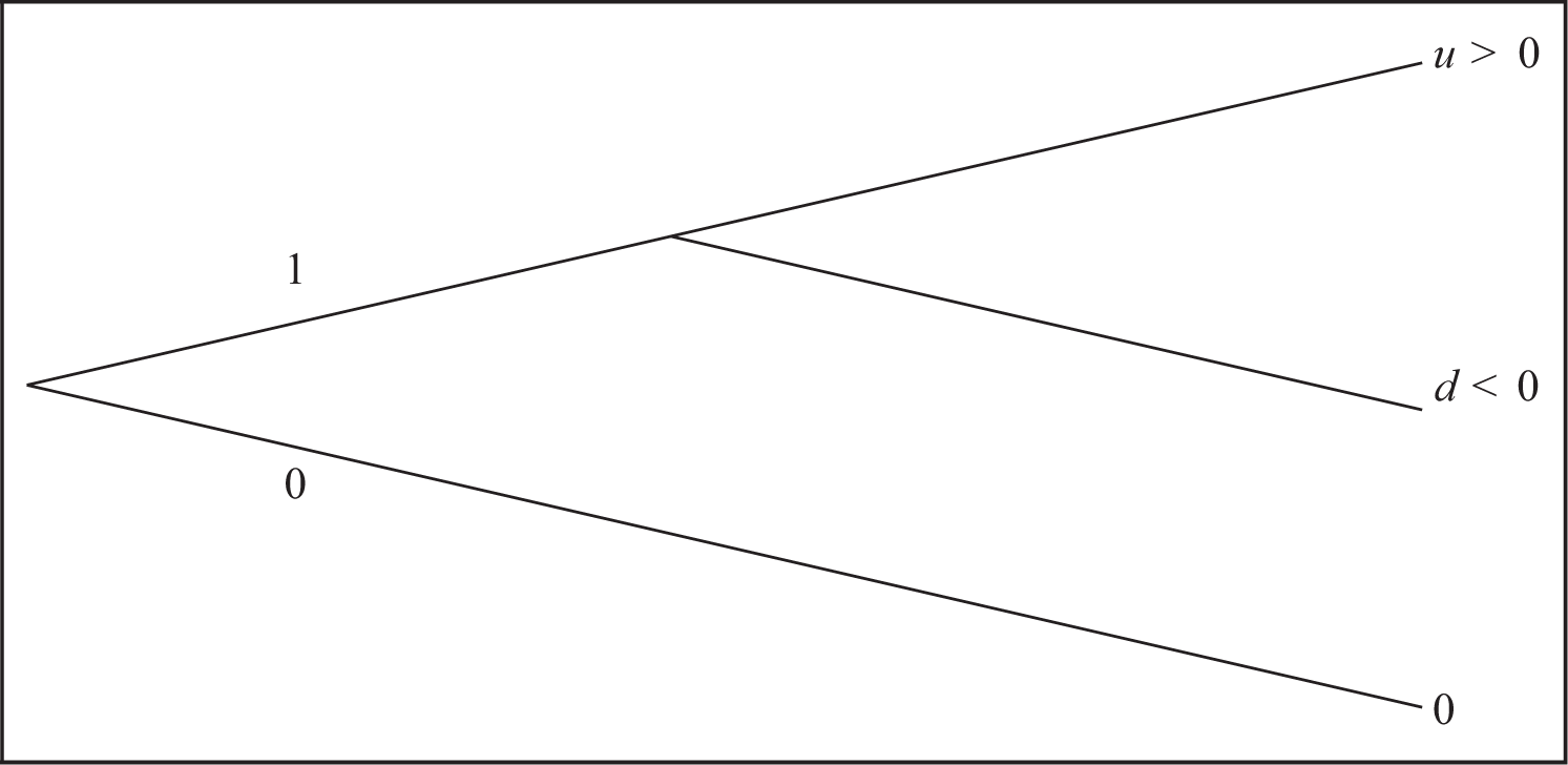
If the firm chooses entry (1), its payoff will be either u > 0 or d < 0, and if it chooses inactive (0), its payoff will be 0. The state is drawn before the DM observes it and makes a choice. The problem is that the DM cannot perfectly observe the state because of scarcity of attention; therefore, it has to arrange to acquire a signal s at a cost by paying λI (s) in order to obtain the information that is most relevant to this choice problem. Then, this knowledge about ε ∈ {u, d} is updated via the posterior rs and 1 − rs. Given the posterior, the DM chooses the action with the highest expected payoff. Let 
Therefore, this solution concept (the information strategy and the ultimate choice behaviour as the essence of this psychological process) can account for when a payoff shock is drawn, what aspects of information about the payoff shock a rationally inattentive agent can and should pay attention to and what choice should be made contingent on this information. The expectation operator sums over possible states ε ∈ {u, d}, possible signals s and possible action choice decisions under the firm’s prior probability distribution, which is that payoff shock u happens with probability p and payoff shock d happens with probability 1 − p. λ > 0 is the cost per unit of information of being more informed when making the action choice decision. This design problem is solved from an ex ante perspective: players must decide how to allocate their attention, which determines what kind of signal players will observe under various circumstances, before learning anything about the current state.
Main Results of Rational Inattention Binary Choice Problem
Here, we summarise Matĕjka and McKay (2015)’s main results of the decision problem. They are expressed in the binary choice context as shown in Figure 1.
The first result of this binary choice problem is that under an optimal information structure
Second, about the choice behaviour, we find that given other primitives, there exists a boundary value of λ denoted by
Define fDP := w(0, λ), FDP (λ) := S(λ, 0), GDP (λ) := T (λ, 0) and µDP := e(0), where the expres sions of w(x, λ), S(λ, x), T (λ, x) and e(x) are given in Appendix A. The analytical expression of 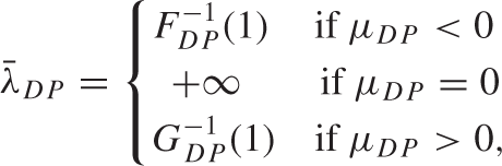
where µDP = pu + (1 − p)d. In addition, define the following function:
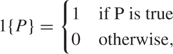
Therefore, Proposition 1 is stated as follows.

Alternatively, the choice probability can be written in a simplified form as

In Proposition 1, the exponential functions in fDP come from the entropy function. At
The Relationship of Rational Inattention Discrete Choice Model and Statistical Decision Problems
Rational inattention discrete choice problems and statistical decision problems (SDPs) are different problems, although the components of these problems (e.g., utility functions, signal, state and prior) are the same. The differences are reflected by two points: (a) an SDP is given the joint distribution of signal and state and the prior distribution of state to derive the optimal decision rule, while a rational inattention discrete choice problem is given the optimal decision rule and the prior distribution of state to obtain the optimal information structure (the joint distribution of signal and state); and (b) in rational inattention binary choice problems, the optimal strategy should contain two signals indicating two different action choices, otherwise more elaborate signals are redundant and hence undesirable. The same rationale applies to rational inattention multiple choice problems. In SDPs, the dimension of signal space is not necessarily equal to the dimension of action space. For binary action problems, it allows more than two signals. However, at the optimum, agents can always divide the signal set into two subsets with respect to the two different action choices.
Therefore, rational inattention discrete choice problems and SDPs can be regarded as the same question but viewed from two different perspectives. A rational inattention discrete choice problem is the ‘reinterpretation’ of an SDP.
Main Results of the Rational Inattention Bayesian Game
In this article, we are interested in agents’ strategic choice behaviour if scarcity of attention exists. We examine this subject in a 2 × 2 incomplete information entry game and focus on the pure strategy Nash equilibrium. In industrial organisation literature, entry games are typically of strategic substitutes, so is our game. By extending the rational inattention approach into a 2 × 2 strategic substitutes incomplete information game, we establish a model that allows us to study how information cost affects an agent’s strategic choice behaviour. Here, we present a summary of the main results of this article.
First, assuming both players’ information costs are identical, we find that there exists a critical value of information cost. 2 If the given information costs of both players are below this value, the game is a Bayesian game, in which the payoff of being active is the production profit plus the private payoff shock. If the given information costs of both players are above or equal to this value, the game becomes a complete information game, in which the payoff of being active is the production profit plus the mean of the distribution of payoff shocks, and players’ best responses are made without acquiring information given any strategy of the opponent.
Next, by studying symmetric games, we find that scarcity of attention can generate multiple equilibria, and that different values of information costs lead to different numbers of equilibria. 3 A general rule is that jointly increasing both players’ information costs first increases and then decreases the number of equilibria. Specifically, in the symmetric rational inattention Bayesian games, we find that given other primitives, by jointly raising the information costs from 0 to +∞, the number of equilibria appears in the following sequence: 1 → 3 → 5 → 3 if multiple equilibria can arise. Alternatively, there always exists a unique equilibrium for any value of the information cost. Besides, we find that in any multiplicity situation, there always exists one pair of asymmetric equilibria in which at least one player plays without acquiring information and relies on their prior knowledge. These results about the game’s equilibria are mainly caused by the concavity–convexity property of the part of the second iteration of the best response functions in which both players play the game by acquiring information. Furthermore, the concavity–convexity property is ultimately induced by the structure of entropy functions. 4 Thus, because information processing capacity is modelled by the reduction in the entropy of players’ posterior over the state space relative to the prior distribution, there are at most five ways to play the game. For any result, it is either that both players make choices by acquiring information or that one player makes choices by acquiring information and the other player makes choices without acquiring information and only relying on prior knowledge.
For comparative statics of equilibrium strategies, we find that in the symmetric equilibrium and outer asymmetric equilibrium, any improvement in players’ expected payoff of entry can increase the probability of entry. 5 If we jointly increase both players’ information costs, its impact depends on the relative magnitude between the prior probability of high payoff shock and a threshold value. If the prior probability of high payoff shock is higher (or lower) than the threshold value, increasing the information cost will increase (or decrease) the probability of entry. If the prior probability of high payoff shock equals the threshold value, increasing the information cost does not have any impact on the probability of entry. There is no conclusive result about comparative statics of inner asymmetric equilibrium without particular parameter specification. Finally, in any equilibrium, if we change only one player’s information cost, its impacts on both players’ equilibrium strategies are not clear without particular parameter specification, but it is found that its impact on one player’s strategy is always opposite to its impact on the opponent’s strategy.
We also study how information cost affects a player’s expected payoff. A player’s information cost does not have any impact on the player’s expected payoff, but the opponent’s information cost can affect the player’s expected payoff through the player’s belief towards the opponent’s behaviour. Except particular parameter specification, there is no conclusive result about at what value of opponent’s information cost, the player’s expected payoff reaches its highest value.
Finally, we study a game in which the players observe their private payoff shocks with an additive noise that follows Type I extreme value distribution. The solution concept is therefore (Bayesian) Quantal Response Equilibria (QRE). The similar looking strategic choice models motivate us to further consider under what conditions the two games can be identical. It is found that there exists a specific set of parameter specification under which both games have a common equilibrium
The rest of this article is organised as follows. The next section describes the model. The fourth section analyses three particular cases of the game with some special value of information cost. The fifth section analyses the general case. The sixth section studies the impact of information cost on players’ best responses. The seventh section presents the equilibria set of the game. The eighth section studies the impact of information cost on players’ equilibrium strategies. The ninth section studies how information cost affects a player’s expected payoff of entry. The tenth section compares a Bayesian quantal response equilibrium game and the rational inattention Bayesian game to determine under what conditions the two types of games can coincide or be identical. The eleventh section concludes this article.
The Model
We study rationally inattentive players’ strategic choice behaviour in the following Bayesian game. Two firms decide whether to enter a market. If a firm enters, it can either get a monopoly profit or a duopoly profit, plus an exogenous payoff shock drawn by nature at the beginning of the time. Each player’s payoff shock is independent from each other, and it is the private information for each player. Each firm can only know its own payoff shock. However, although a firm has full access to its own payoff shocks, due to scarcity of attention, it is only able to possess partial information about some aspects of the payoff shock, and this information is obtained by acquiring a signal at a cost. What kind of signal a player (firm) will observe is unconsciously designed in their mind and the player only acquires information about their own shock. A player cannot acquire any information about the opponent’s private payoff shock because it is the opponent’s private information and it is independent from the player’s own payoff shock. Both players make decisions according to observed private signals.
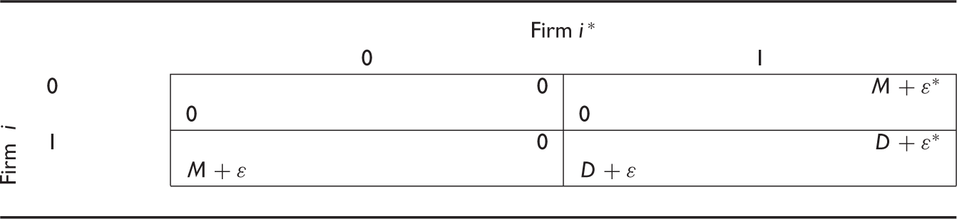
We define our game as follows. The firms’ strategic entry behaviour is characterised by the 2 × 2 Bayesian game with payoffs shown in Table 2.
We use ∗ to denote all variables of the opponent. In this article, except in some particular situations, for simplicity we do not describe i∗’s specification separately and its specifications are correspondingly symmetric with i’s. Here, ε ∈ {u, d} is i’s private payoff shock, and ε∗ ∈ {u, d} is opponent i∗’s payoff shock. Assume u > d. The shocks ε and ε∗ have the same distribution, namely p = Pr(u) and 1 − p = Pr(d), and we assume that ε and ε∗ are independent and p ∈ (0, 1). The payoff shocks are private information for each player. Nature draws ε and ε∗, respectively, for the players at the beginning of the time, and since they cannot perfectly observe ε or ε∗, they have to acquire a signal at cost, which can reveal some aspects of ε or ε∗. To acquire at a cost what type of signals is designed by each player, the efficient signal should undoubtedly be the most relevant to the player’s choice decision. We assume that each player’s signal is conditionally independent of the opponent’s signal given the player’s own payoff shock. The true value of the payoff shock can only be known after they make their choices. The action set of player i is A = {0, 1}, where 1 stands for ‘entry’ (being active) and 0 stands for ‘staying outside’ (being inactive). If both firms enter, they will engage in a Cournot competition and each firm gets a payoff D that is strictly lower than the monopoly profit M.
The game exhibits strategic substitutes because when the probability that the opponent chooses entry increases, the marginal expected payoff gain of being active over inactive decreases. 6 Therefore, the opponent’s more aggressive behaviour imposes a negative externality on a player’s marginal payoff.
Now let us turn to discuss what kind of signal they will acquire. As stated above, before selecting an action, both players can privately acquire information about their own payoff shocks at a cost. The root of the inability to grasp the full knowledge about ε or ε∗ is still scarcity of attention, and the information acquisition process in this game is thus modelled in the rational inattention framework. The signal the players intend to acquire is characterised by the set of realisations of player i’s signal, S ∈ R, and the information structure
According to the results of the rational inattention binary choice problem described in the last section, rationally inattentive agent’s optimal information structure just contains two signal realisations because essentially, acquiring more elaborate signal not only is costly but also provides no extra benefit to the player, since the player must always take either action 1 or action 0. Hence, without loss of generality, i’s strategy can be represented by the following function.
That is, when i’s private payoff shock is ε, player i receives signal 1 (signal 0) with probability qε (1 - qε) and then takes action 1 (action 0) as instructed.
Given i∗’s strategy qε∗, player i’s expected payoff of playing qε is

where q∗ = pqu∗ + (1 − p)qd∗. Equation (1) is directly derived from Table 2. As a standard setup in rational inattention literature, the information cost associated with a strategy qε is given by λI (qε), where I (qε) is the amount of information conveyed by qε, and λ > 0 is a scaling parameter that controls the difficulty of acquiring information. Specifically,

where q = pqu + (1 − p)qd. According to the symmetry property of mutual information,
Taking information cost into account, i’s and i∗’s overall expected payoff in terms of qε and 
and

For simplicity, in the rest of this article, we abstract from the story of market entry and deal with the problem simply as a 2 player game with Equations (3) and (4) and strategy profile (qε,
Under Assumption 1, random payoff shocks dominates deterministic payoffs in players’ decision making. If λ = λ∗ = 0, the ex ante choice probability of each action totally depends on the prior distribution, and hence, there exists a unique equilibrium. Therefore, Assumption 1 makes the underlying game a good benchmark to compare games with scarcity of attention. 7
Three Particular Cases
Before we analyse the general game, let us begin from three particular cases: (a) λ = λ∗ = 0; (b) λ = λ∗ = +∞; and (c) λ = 0 and λ∗ = +∞. These particular cases provide useful benchmarks for further analysis. Remember that we only consider pure strategy equilibrium.
In Case 1, signals are free, and hence players can possess full information about private payoff shocks, and this game then comes back to a typical incomplete information game. According to Assumption 1, in such games, there exists a unique Bayesian Nash equilibrium, (q, q∗) = (p, p). Under Assumption 1, given the payoff shock u, a player will certainly choose action 1 and hence qu = 1. Given the payoff shock d, a player will certainly choose action 0 and hence qd = 0. Therefore, the unconditional probability of choosing action 1 is q = pqu + (1 − p)qd and in this situation, the unconditional choice probability is a sufficient statistic to describe the equilibrium.
In Case 2, when λ = λ∗ = +∞, any signal is too costly to acquire. Then, a Bayesian player will make a choice by simply comparing the ex ante expected payoffs for each action, which are the expected payoff before payoff shocks are drawn by nature and are simply formulated based on prior knowledge as well as the opponent’s strategy. Case 2 can be further analysed in three specific situations:
If D + pu + (1 − p)d > 0, then there exists a unique equilibrium (q, q∗) = (1, 1), since under this condition, for all q∗ ∈ [0, 1], (1 − q∗)M + q∗D + pu + (1 − p)d > 0; If M + pu + (1 − p)d < 0, then there exists a unique equilibrium (q, q∗) = (0, 0), since under this condition, for all q∗ ∈ [0, 1], (1 − q∗)M + q∗D + pu + (1 − p)d < 0; If M + pu + (1 − p)d > 0 and D + pu + (1 − p)d < 0, then generically there exist three equilibria (q, q∗) = (1, 0), (0, 1), and
The Strategic Entry Game when λ = λ∗ = +∞.
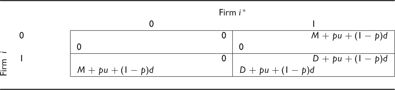
The three generical equilibria in 3 are obtained in this way and in fact, 1 and 2 can also be analysed in this complete information game framework. The equilibria in 1 and 2 are dominant strategies.
Finally in Case 3, λ = 0 and λ∗ = +∞. In this situation, player i possesses full information about their private payoff shock and knows nothing about player i∗’s private payoff shock, while player i∗, as in Case 2, only relies on prior information and knows nothing about player i’s contingent payoff shock either. Then, for player i, the equilibrium strategy is p for the probability of choosing action 1, and hence, 1 − p for the probability of choosing action 0. Correspondingly, player i∗’s equilibrium strategy is a∗ = 1{(1 − p)(M + d) + p(D + u) > 0}. Therefore, in this situation, there still exists a unique equilibrium. Player i’s strategic choice, where λ = 0, depends on contingent payoff shocks, and player i∗’s decision, where λ∗ = +∞, depends only on prior information. Note that 1 in all three particular cases, there is no information acquisition, either because players have perfect observation or because signals are too costly to acquire, and 2 the choice behaviour where a player does not acquire information does not just belong to λ (or λ∗) → +∞. We will show that given the opponent’s strategy q∗ ∈ [0, 1], a player will not make a choice by acquiring information when λ is greater than a certain value, and in this situation, the choice behaviour is just the one we have presented for λ → +∞.
General Case
Now, we deal with the general game. A Nash equilibrium of game G(M, D, λ, λ∗) is a strategy profile (qε,
G 1:
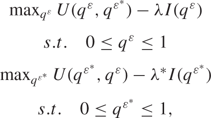
where ε (or ε∗) ∈ {u, d}.
By solving G 1, we obtain two equations that contain qε and 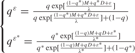
where ε (or ε∗) ∈ {u, d}, and q = pqu + (1 − p)qd and
To obtain (q, q∗), rather than using the relation q = pqu + (1 − p)qd or
G 2:
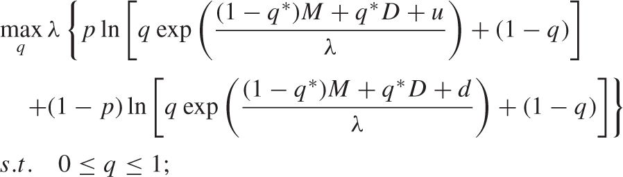
where q and q∗ are strategic choices. We define f (q∗, λ) := w((1 − q∗)M + q∗D, λ). The function w(x, λ) is the same one in the decision problem. If interior solutions exist, we obtain the following best response functions:

for all q∗ ∈ [0, 1], and q∗ = f (q, λ∗) for all q ∈ [0, 1]. We can prove that, given all primitives, the interior solution q from G-2 and corresponding qε from G-1 satisfy q = pqu + (1 − p)qd, so satisfy 
The first equation in Equation (7) is derived from f (q∗, λ) ≥ 0 and the second equation from f (q∗, λ) ≤ 1.
We are interested in given M, D and the prior distribution, the range of λ that ensures the existence of interior solutions of G-2. In this article, for a bivariate function y = f (x, v), its inverse function with respect to x is expressed as x = f −1(y; v). We define µ(q∗) := e((1 − q∗)M + q∗D) = (1 − q∗)M + q∗D + pu + (1 − p)d. It is found that there indeed exists a 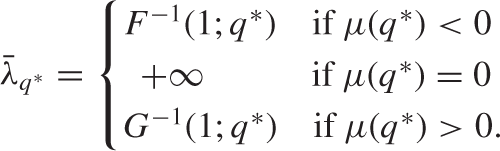
If

Alternatively, the best response function can be written in a simplified form as follows:

The exponential form of f (q∗, λ) comes from the entropy function. At
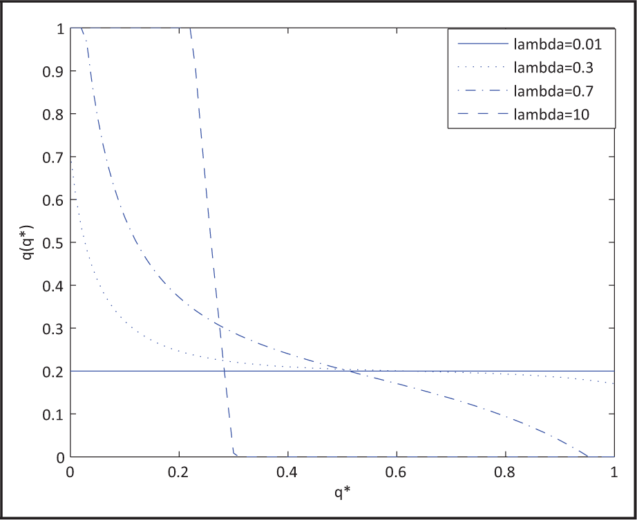
From Proposition 2, we can learn that given a λ > 0, if q(q∗) = f (q∗, λ), the best response function is a decreasing curve with respect to q∗. If q(q∗) = 0 × 1{µ(q∗) < 0} + 1 × 1{µ(q∗) > 0}, the best response function is a horizontal line with respect to q∗. In addition, given Assumption 1, it is found that
Since this game exhibits strategic substitutes, it is not surprising that the best response function is non increasing. The best response function can reflect two distinct strategic choice behaviour: one by acquiring information, represented by the curvature part of the best response function, and another by comparing ex ante expected payoff of each action, represented by the horizontal parts of the best response function. Only prior knowledge matters for the latter approach. Therefore, the best response of a player in this game reflects not only the player’s rational choice of an action but also their choice of behaviour, that is, the decision is made whether by acquiring information or by comparing ex ante expected payoff of each action.
To conclude this section, we exhibit some numerical examples of the best response function. In these examples, we maintain the values of M, D, u, d, p constant and only change the value of λ from 0.01 to 10. From Figure 2, we see that when λ is large enough, some parts of the best response function become horizontal, which indicates that given the relevant opponent’s strategy, a player’s best response is made without paying heed to any contingent information and just relying on the prior knowledge (see Figure 2).
The Impact of Information Cost on a Rational Inattentive Player’s Best Response
For the comparative statics analysis in this section, we focus on the case that q ∈ (0, 1) given q∗ ∈ [0, 1]. That means a player’s best response is made by acquiring information. In fact, it is not interesting to investigate the boundary cases (q = 0 or q = 1). If q = 1, there is no scope of increasing it further. If q = 0 and
By increasing M, D, u and d, the expected payoff of entry increases, and hence q(q∗) increases given q∗ ∈ [0, 1]. If p increases, the high payoff shock u will happen more often, and it encourages the player to choose entry. Therefore, q(q∗) increases as p increases given q∗.
We define
To intuitively understand Proposition 3, we have to resort to the analytical expression of 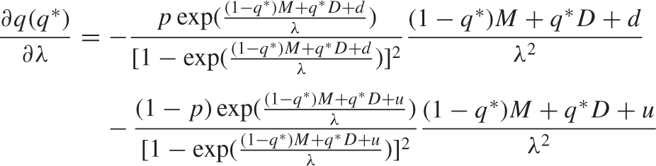
The parameter λ converts bits of information to utils. Therefore,
To interpret the second result in Proposition 3, we can use the chain rule, according to which the impact of λ on the opponent’s best response, q∗(q), can be decomposed as
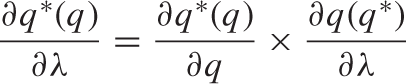
Therefore, the impact of λ on q∗(q) can be decomposed into two separate effects:
The Equilibrium
Proposition 2 implies that the best response function is continuous with respect to the opponent’s strategy. Therefore, according to Brouwer’s fixed point theorem, we obtain the following proposition.
We use parenthesis to denote the word ‘Bayesian’ because there exists a critical value λ = λc, and for λ > λc, the game turns into a complete information game. We will show this in detail later in Proposition 6.
Dominance Solvability
The next question is under what conditions the game is dominance solvable. If the game is dominance solvable, the game will exhibit a unique equilibrium. A sufficient condition to ensure that the game is dominance solvable is that both players’ best response functions are contraction. Therefore, we have the following proposition.
f (q∗, λ) is expressed by Equation (6).
Now, we look at the intuition of Proposition 5. According to our proof, it is found that the lowest value of
If
Given a q∗ ∈ [0, 1], it is found that as λ increases from 0,
From a Bayesian Game to a Complete Information Game
From ‘General Case’ section, it is found that when the information cost is too high, a player’s best response will be made by comparing ex ante expected payoff of each action. Nevertheless, the game may still be a Bayesian game since the player’s best response towards some other strategies is still made by acquiring information. However, the game can turn into a complete information game where λ is higher than some critical value. We obtain the following proposition.
From Proposition 2, it is known that given
Further, we determine the analytical expression of λc. They are given by the following corollary.
µ(q∗) is as defined in ‘General Case’ section. F (λ, q∗) and G(λ, q∗) are expressed by Equation (7).
Equilibria of the Game
Here we give a complete characterisation of the equilibrium set of the game for all parameter specifica tions. It is given by Proposition 7.
Under some parameter specifications, there exist λ1 and λ2 such that 0 < λ1 < λ2 < λc. ∀λ ∈ [0, λ1), there is a unique equilibrium. At λ = λ1, there are three equilibria. ∀λ ∈ (λ1, λ2), there are five equilibria. ∀λ ∈ [λ2, λc), there are three equilibria.
∀λ ∈ (0, λ2), the symmetric equilibrium is stable. 9 At λ = λ2, the stability of the symmetric equilibrium cannot be determined. ∀λ ∈ (λ2, λc), the symmetric equilibrium is unstable.
Otherwise, under some parameter specification satisfying µ(q∗ = 0) < 0 or µ(q∗ = 1) > 0, there is a unique equilibrium ∀λ ∈ [0, λc), which is stable.
In the following, we explain Proposition 7. The equilibria are solutions of an equation group comprising the 2 players’ best response functions. By putting the opponent’s best response function into i’s best response function, we get the following function with respect to q, which is the second iteration of the best response functions, g(q∗(q)):

where 
Geometrically, Equation (10) shows that the equilibria are intersection points between 45◦ line and g(q∗(q)). g(q∗(q)) and A(q∗(q)) are continuous and non decreasing with respect to q for all λ ∈ (0, +∞). Because the game is symmetric and best response function q∗(q) is non increasing, there always exists a unique symmetric equilibrium. In addition, if asymmetric equilibria exist, one asymmetric equilibrium always has a corresponding equilibrium obtained by switching players’ identities. Therefore, in such games, asymmetric equilibria always appear in pairs and hence the total number of equilibrium is odd.
We define set h := {q|0 ≤ f (q, λ∗) ≤ 1 and 0 ≤ A(q∗(q)) ≤ 1}. A(q∗(q)) of q ∈ h represent the part of A(q∗(q)) that is between 0 and 1 and no horizontal parts. Its economic sense is that both players’ best response functions are made by acquiring information. The horizontal parts of g(q∗(q)) indicates that there is at least one player not playing the game by acquiring information. It is proven that when multiple equilibria arise, as q increases, g(q∗(q)) where q ∈ h first exhibits concavity until q = τ , and then exhibits convexity afterwards, where τ ∈ (0, 1). Therefore, we call this property as concavity–convexity property of A(q∗(q)).
In addition, we denote the symmetric equilibrium of the Bayesian game by (s, s). It can be found that s ∈ h. This is because the Bayesian game exhibits strategic substitutes, and the best response function is non increasing and not constant. Therefore, in the Bayesian game, there is no equilibrium like (0, 0) or (1, 1). Hence, in the symmetric equilibrium, both players always make decisions by acquiring information.
We define set k := {q|0 ≤ f (q, λ∗) ≤ 1}. The last component we need in order to explain Proposition 7 is that
Multiple Equilibria with Stable Symmetric Equilibrium
When λ is small, the game is dominance solvable and the symmetric equilibrium (s, s) is stable. Thus, at
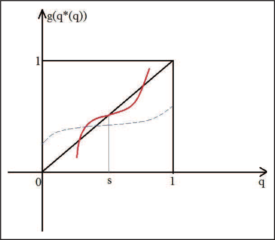
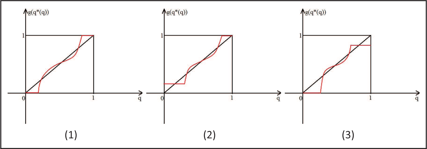
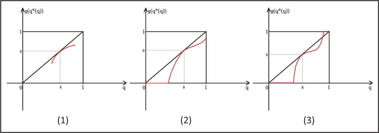
To complete the solid curve in Figure 3 as the geometric representation of g(q∗(q)) with respect to q ∈ [0, 1], we should draw two horizontal lines at the two sides of A(q∗(q)) of q ∈ h. According to the symmetry property of the game, there are three possible situations of a complete g(q∗(q)) curve. They are determined by whether g(q∗(0)) = 0 or not, or g(q∗(q)) = 1 or not. Irrespective of the possible situation, g(q∗(q)) will have five intersection points with the 45◦ line (see Figure 4).
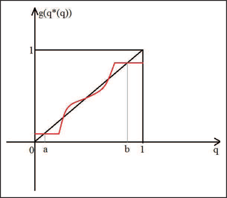
Situations such that shown in Figure 5 cannot happen. Figure 5 is characterised by g(q∗(0)) > 0 and g(q∗(1)) < 1. In Figure 5, (a, b) and (b, a), where a, b ∈ (0, 1), form a pair of asymmetric equilibria in which both players make their equilibrium strategies by acquiring information. However, the intersection points a and b are made by the horizontal part of g(q∗(q)) and the 45◦ line. It implies that there is at least one player not acquiring information, and hence that player’s strategy (a or b) is either 0 or 1. However, both a and b are between 0 and 1. Hence, a contradiction arises, and (a, b) and (b, a) in Figure 5 cannot be equilibria of the symmetric rational inattention Bayesian game. Thus, if there are five equilibria, only the three situations in Figure 4 are the correct situations.
At the boundary situation (λ = λ1), where the game transits from a unique equilibrium situation to five equilibria situation, according to the concavity–convexity property and
From Figure 6, we can see that if we slightly increase λ to λ1 + ε, where ε > 0 is an arbitrarily small number, since
Therefore, as long as the symmetric equilibrium is stable, there are at most five equilibria in this game.
Multiple Equilibria with Unstable Symmetric Equilibrium
As λ increases, according to
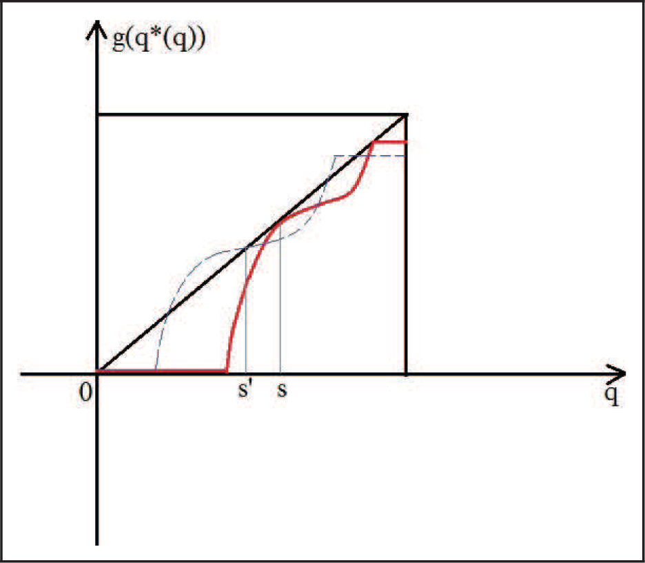
Suppose that
From Figure 7, we can see that if the symmetric equilibrium is tangent with the 45◦ line, the number of equilibria will be even. Therefore, a contradiction arises.
In addition, situations indicated by Figure 8 also cannot happen. In Figure 8, the stability of the symmetric equilibrium is not determined and there are three equilibria. However, if λ increases to λ2 + ε, because
Therefore, at λ = λ2,
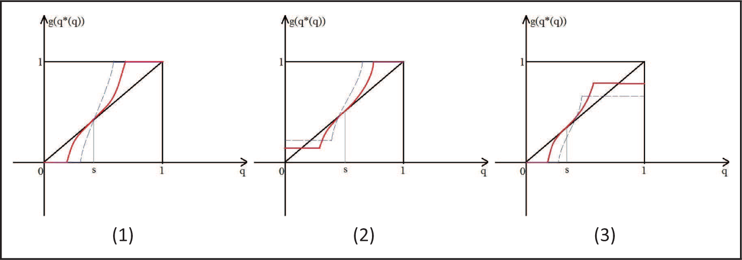
Because
Therefore, if players with scarcity of attention play the Bayesian game of Table 2 and the scarcity of attention is modelled by the reduction in the entropy of players’ posterior over the state space relative to the prior distribution, there are at most five ways to play the game. For any result, either both players make choices by acquiring information or one player makes choices by acquiring information and the other player makes choices without acquiring information and relying only on prior knowledge.
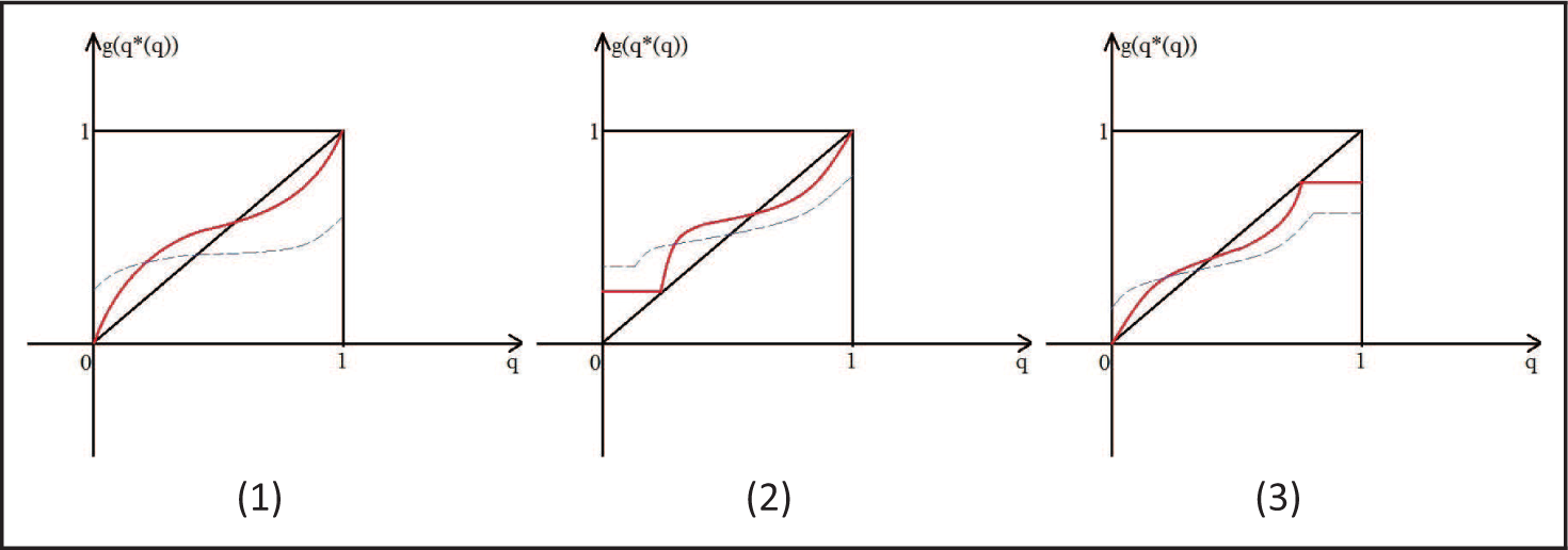
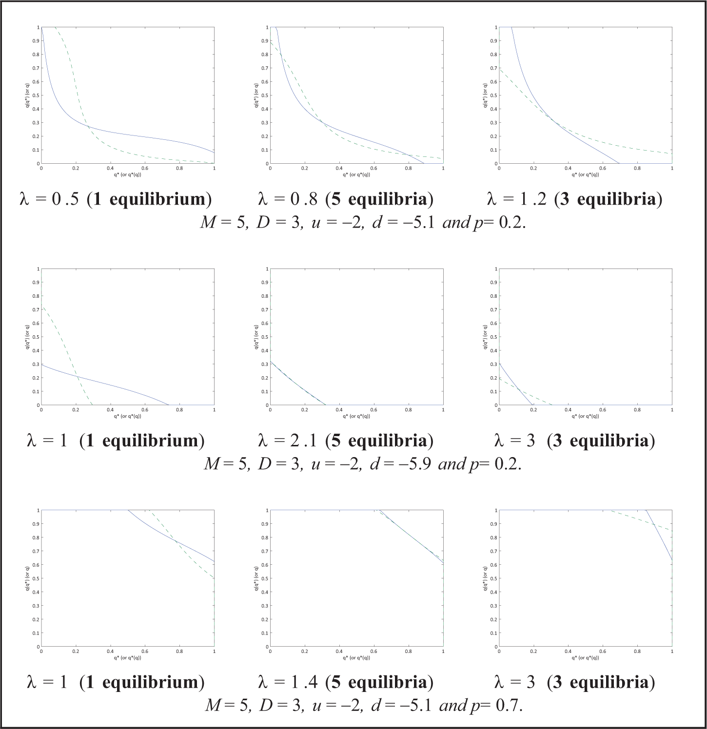
To conclude ‘Multiple Equilibria with Stable Symmetric Equilibrium’ and ‘Multiple Equilibria with Unstable Symmetric Equilibrium’ sections, we present some numerical examples to visually exhibit how different number of equilibria arise. They are presented in Figure 10. The three figures in the first row represent the situation in which µ(q∗ = 0) > 0 and µ(q∗ = 1) < 0. The three figures in the second row represent the situation in which µ(q∗ = 0) < 0. The three figures in the third row represent the situation in which µ(q∗ = 1) > 0. We can see that in any situation, the number of equilibria in each row of numerical examples follows the 1-5-3 sequence as λ increases (see Figure 10).
The Explanation of Result (2) in Proposition 7
Logically, under any parameter specification, as λ increases from 0, the game may exhibit a unique equilibrium, or not, for all λ ∈ (0, +∞). Result (1) in Proposition 7 belongs to the ‘or not’ part.
For some parameter specifications satisfying µ(q∗ = 0) < 0 or µ(q∗ = 1) > 0, the game contains a unique equilibrium for all λ ∈ (0, +∞). We can find numerical examples to support this fact:
µ(q∗ = 0) < 0: p = 0.2, M = 5, D = 3, u = −2 and d = −10; µ(q∗ = 1) > 0: p = 0.8, M = 2, D = 1, u = 1 and d = −2.01.
Therefore, if µ(q∗ = 0) < 0 or µ(q∗ = 1) > 0, it is possible that there is only one way for both players with scarcity of attention to play the Bayesian game shown in Table 2. In this situation, both players will acquire information to make decisions.
However, if parameters satisfying µ(q∗ = 0) > 0 and µ(q∗ = 1) < 0, multiple equilibria will surely happen when λ is large enough. For all
Hence, in the case of µ(q∗ = 0) > 0 and µ(q∗ = 1) < 0, as λ increases from 0, a player’s best response q(q∗) will rise to 1
Impact of Information Cost on Equilibrium Strategy
In the symmetric strategic substitutes game, the symmetric equilibrium always exists and is unique. When multiple equilibria arise, there are two types of asymmetric equilibria. In one type, there is at least one player choosing action 0 or 1 by comparing ex ante expected payoff of each action. This type of asymmetric equilibria is usually located at the outer part of a player’s best response function, hence named outer asymmetric equilibria. In the other type, both players make their best response by acquiring information. This type of asymmetric equilibria is usually located at the inner part of a player’s best response function, hence named inner asymmetric equilibria.
For outer asymmetric equilibria, according to the payoff specification, there are three specific results:
If µ(q∗ = 0) > 0 and µ(q∗ = 1) < 0, they are (1, 0) and (0, 1); If µ(q∗ = 0) < 0, they are (t, 0) and (0, t), where t ∈ (0, 1); If µ(q∗ = 1) > 0, they are (j, 1) and (1, j), where j ∈ (0, 1).
In an equilibrium, if a player always chooses 0 or 1 deterministically, the corresponding comparative statics results with respect to any parameter are always equal to 0. Only the equilibrium strategy that is made by acquiring information, that is, q ∈ (0, 1), will be further analysed.
For inner asymmetric equilibria, there are no conclusive comparative statics results. It depends on particular parameter specifications.
The intuition of Proposition 8 is that increasing τ ∈ {M, D, u, d, p} can increase the expected payoff of entry; therefore, a player is more willing to choose entry. If q∗ = 0 and µ(q∗ = 0) = M + pu + (1 − p)d < 0, duopoly cannot happen, and hence,
For Proposition 9, it is found that at symmetric equilibrium (s, s),
Finally, for any type of equilibrium, what is the effect of the situation where only one player’s information cost changes given the other parameters? The answer is that the impact of changing one player’s information cost on both players’ equilibrium strategy cannot be determined without particular parameter specification in any equilibrium. We define

and
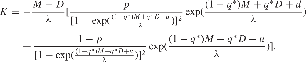
The signs of H and K could be positive or negative. It is found that

and

The signs of 1 − HK and
Impact of Information Cost on Players’ Expected Payoffs of Entry
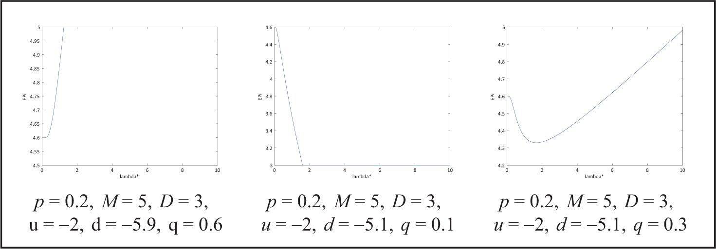
In this article, we have two types of expected payoff of entry: the ex ante expected payoff of entry, that is, (1 − q∗)M + q∗D + pu + (1 − p)d, and the typical expected payoff of entry, that is, (1 − q∗)M + q∗D + ε, where ε ∈ {u, d}. For both types, λ or λ∗ can only affect (1 − q∗)M + q∗D. We define 
and hence,

Because if and only if
(Bayesian) Quantal Response Equilibrium and Rational Inattention Bayesian Nash Equilibrium

The players make their decisions after observing their respective private payoff shocks ε and ε∗. However, the observation is always affected by an additive error η (or η∗). Therefore, what they actually observe is ε + η and ε∗ + η∗, assuming that η is independent from η∗. Assumption 1 in ‘The Model’ section is still held in this game. Therefore, if player i observes u + η or d + η, in this game, the player’s choice is probabilistic because D + u > 0 > M + d. The solution concept of this game is therefore (Bayesian) Quantal Response Equilibrium (QRE) (McKelvey & Palfrey, 1995).
It is assumed that η follows Type I extreme value distribution, that is, 
Let us recall the conditional choice probability in the rational inattention Bayesian game. Given q∗ ∈ [0, 1] and 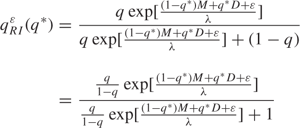
Since Equations (11) and (12) look similar, it is natural to ask under what parameter specifications Equations (11) and (12) are identical. If they are identical, there will be a clear economic and psycho logical justification of why the disturbances η should be extreme value distributed in the Bayesian QRE game.
It is found that if and only if

where
The best response function of the Bayesian QRE game is given by

Given q∗ ∈ [0, 1], qQRE ∈ (0, 1). As α → +∞, the Bayesian QRE game converges to the benchmark Bayesian game, which is also the limit of the rational inattention Bayesian game as λ → 0. In this situation, qQRE = p. As α → 0, in the Bayesian QRE game, actions consist of all observational errors such that all actions become indifferent ex ante. Hence,
Therefore, in conclusion, if there is a set of parameters satisfying
Conclusion
In this article, we have studied how scarcity of attention affects economic agents’ strategic choice behaviour in an incomplete information environment. We use the rational inattention approach to model scarcity of attention. Given the opponent’s strategy, as the information cost changes from 0 to +∞, a player’s behaviour of making best responses will switch from by acquiring information to by com paring ex ante expected payoff of each action. The latter behaviour solely relies on the player’s prior
knowledge. This behaviour transition is the behavioural manifestation of the mathematical property that the continuity of the best response function with respect to the opponent’s strategy is always ensured no matter how λ changes. Hence, the best response function indeed contains two distinct choice behaviours.
It is particularly interesting to determine the impact of attention scarcity on forming equilibria and affecting players’ strategic behaviour. By studying symmetric games, we find that scarcity of attention can bring multiple equilibria and it is the high information cost that generates multiple equilibria. The number of equilibria differs with respect to different ranges of information cost. In any multiplicity situation in symmetric games, there always exists one pair of asymmetric equilibria in which at least one player plays the game without acquiring information.
In a symmetric equilibrium or an outer asymmetric equilibrium (q, q∗), the effect of attention scarcity on a player’s information acquisition choice behaviour depends on whether p is greater than
Finally, we have compared the rational inattention Bayesian entry game with a Bayesian QRE entry game. It is found that there exists a set of parameters satisfying
For future research, we will study the situation that players pay full attention to their own information but are inattentive to their opponents’ information. We are interested in how players make their strategic choices in such a paradigm. In future study, we will investigate this problem to see how players’ behaviour deviates from the behaviour in the game in which scarcity of attention exists for players to their own information.
Supplementary Material
Supplementary Files are available online for this article.
Footnotes
Acknowledgement
This article is the final chapter of my PhD thesis at University of Edinburgh. I thank Tim Worrall, Andy Snell, Jonathan Thomas, Subir Bose and Jozsef Sakovics for their helpful comments to improve this article.
Declaration of Conflicting Interests
The author declared no potential conflicts of interest with respect to the research, authorship and/or publication of this article.
Funding
This work was supported by Economic and Social Research Council (ESRC) of United Kingdom. The author received a 3 year doctoral fellowship (2012–2015) from ESRC, which the author gratefully acknowledges.
Notes

References
Supplementary Material
Please find the following supplemental material available below.
For Open Access articles published under a Creative Commons License, all supplemental material carries the same license as the article it is associated with.
For non-Open Access articles published, all supplemental material carries a non-exclusive license, and permission requests for re-use of supplemental material or any part of supplemental material shall be sent directly to the copyright owner as specified in the copyright notice associated with the article.
