Using residualized change versus difference scores for longitudinal research

Abstract

Researchers interested in studying change over time are often faced with an analytical conundrum: Whether a residualized change model versus a difference score model should be used to assess the effect of a key predictor on change that took place between two occasions. In this article, the authors pose a motivating example in which a researcher wants to investigate the effect of cohabitation on pre- to post-marriage change in relationship satisfaction. Key features of this example include the likely self-selection of dyads with lower relationship satisfaction to cohabit and the impossibility of using experimentation procedures to attain equivalent groups (i.e., cohabitants vs. not cohabitants). The authors use this example of a nonrandomized study to compare the residualized change and difference score models analytically and empirically. The authors describe the assumptions of the models to explain Lord’s paradox; that is, the fact that these models can lead to different inferences about the effect under investigation. They also provide recommendations for modeling data from nonrandomized studies using a latent change score framework.

Keywords

ANCOVA difference scores latent change scores latent difference scores longitudinal analysis Lord’s paradox residualized change

Sofia, a close relationships’ researcher, is interested in examining change in relationship satisfaction before and after marriage. Specifically, she wants to know whether cohabiting prior to marriage has an effect on changes in relationship satisfaction. As she plans her data analysis strategy, Sofia realizes she has two options: (1) use the postmarriage relationship satisfaction score as her outcome and include the premarriage score in her analysis as a predictor, in addition to whether or not couples cohabited prior to marriage to account for individual differences in baseline relationship satisfaction (known as residualized change approach) or (2) compute the difference between the postmarriage relationship satisfaction score and the premarriage relationship satisfaction score and use it as her outcome to test the effect of cohabiting prior to marriage (known as difference score approach). Which of these two strategies is most appropriate? Should both strategies provide the same results? Sofia has heard difference scores have a bad reputation, why is that? Are there additional strategies Sofia is not aware of that might be preferred over her current options?

The questions outlined above are at the heart of this article. Close relationship researchers, as many others in the social sciences, are likely to have encountered similar questions when conducting longitudinal research. The answers to these questions, however, have not always been clear. In this article, we share our view of the issues raised by the use of residualized change and difference score models. Our goal is to give specific and simple examples that will aid close relationship researchers when conducting longitudinal analyses and choosing between these two approaches. Importantly, there is a body of literature that has shed light on the issues we discuss here (Eriksson & Häggström, 2014; Gollwitzer, Christ, & Lemmer, 2014; Gottman & Rushe, 1993; Liker, Augustyniak, & Duncan, 1985; Lord, 1967; Maris, 1998; Pearl, 2014; van Breukelen, 2013; Wainer, 1991), and we encourage those seeking additional examples or perspectives to consult this literature.

We start by explaining why difference scores have gained a bad reputation in the field. Then, we define the two strategies that our fictional researcher, Sofia, can use for conducting her analysis. We continue by relying on these definitions to compare the approaches analytically and through empirical illustration using simulated data that map on to our example in the opening paragraph. Finally, we describe the role of measurement error in choosing between models and finish by describing the latent change score (LCS) framework, which provides close relationship researchers with what we consider is an ideal alternative for studying change in longitudinal studies. Throughout the article, there are important take-home messages for applied researchers. We summarize these at the end of our discussion for those who want a straightforward answer to the guiding questions above. Finally, we include R and Mplus code in the Appendix to replicate all analyses presented in the article.

Bad reputation of difference scores: Where did it come from?

If psychological tests were perfectly reliable, there would be no need for further discussion, since the best estimate of a pupil’s gain would be obtained by the obvious procedure of subtracting his [sic] score on the first test from his score on the second. The fact that test scores are not perfectly reliable often makes this “obvious” procedure produce absurd results. (Lord, 1956, p. 421)

…there is a need for a sound method for estimating the “true gain” of each pupil, that is, to obtain an estimate of his [sic] gain from which any bias due to errors of measurement has been eliminated insofar as possible. (Lord, 1956, p. 424)

Frederic Lord made great contributions to the study and measurement of change and was one of the first to point to the negative consequences measurement error can have for accurately assessing change. Indeed, from a classical test theory perspective, the difference between two imperfectly measured observed scores results in an amalgam of true score change and change in measurement error. When not much true score change has occurred (low variability in true score change), this can have serious implications for the reliability of difference scores (Lord, 1956). In addition, Lord (1956) pointed to the issue of comparing difference scores across units of assessment (e.g., dyads) who start at different levels of a scale. These comparisons can be meaningless unless one can demonstrate a scale has equal intervals at different levels, suggesting that a one-unit increase for someone who started with a low score is equivalent to a one unit increase of someone who started with a high score on the scale.

These and other issues (e.g., the decreased variability of difference scores) were further emphasized in a seminal article whose title says it all: “How we should measure “change”—or should we?” (Cronbach & Furby, 1970). In this article, very strong statements against using difference scores were made:
“Raw change” or “raw gain” scores formed by subtracting pretest scores from posttest scores lead to fallacious conclusions, primarily because such scores are systematically related to any random error of measurement. Although the unsuitability of such scores has long been discussed, they are still employed, even by some otherwise sophisticated investigators. (Cronbach & Furby, 1970, p. 68)
Sophisticated or not, this message (presented on the opening paragraph of Cronbach and Furby’s article) would make researchers, at least, think twice about the appropriateness of computing difference scores for analyses. The main criticism in this article was yet again centered on the imperfect reliability of scores, and thus, the potential abysmal reliability of difference scores. Cronbach and Furby (1970) reviewed several approaches that were available at that time for capturing change and concluded that, “It appears that investigators who ask questions regarding gain scores would ordinarily be better advised to frame their questions in other ways.” (p. 80). Their advice stuck with many for years until Rogosa and colleagues demonstrated that investigations about the reliability of difference scores had only considered extreme and unusual assumptions about the true change among individuals (Rogosa, Brandt, & Zimowski, 1982; Rogosa & Willett, 1983). For example, Cronbach and Furby (1970) assumed strong correlations between baseline scores and subsequent change, yet Rogosa and Willett (1983) revealed that with lower correlations, the reliability of difference scores would be much higher than previously shown.

Rogosa and colleagues rehabilitated the standing of difference scores in the literature, although they advocated for collecting more than two assessments of data in any longitudinal investigation to maximize the information obtained from each unit of analysis. In an attempt to disseminate Rogosa and colleagues’ contributions regarding the study of change, Gottman and Rushe (1993) reviewed previously encountered myths surrounding the use of difference scores. Among other things, they reminded psychologists that difference scores could be reliable. Nevertheless, whether difference scores have shaken off their bad reputation over the years is questionable, as researchers affirm encountering pushback when using difference scores in their research (Gollwitzer et al., 2014).

Moreover, with the advent of structural equation modeling (SEM)—which permits modeling of error-free constructs—much of the criticism against difference scores in the literature has decayed further. Advances in SEM make the specification of latent difference scores possible (McArdle & Nesselroade, 1994), and these models can be particularly helpful when multiple indicators are used and a perfectly reliable difference score can be specified (e.g., Henk & Castro-Schilo, 2016). We discuss latent difference scores (aka LCS) in a later section of this article.

In sum, there are strong arguments advocating the use of difference scores, especially if these are latent. But if this information is not salient to researchers like Sofia, then they are likely to be uncertain on how to proceed with their analyses of longitudinal data. As Sofia ascertained, with her pre- and posttest design, there are two analytic options that are likely to come to mind: a residualized change model and a difference score model.

The residualized change approach

When researchers use the term residualized change, they refer to one of two well-known models for two-occasion data: the analysis of covariance (ANCOVA) model or the multiple regression model. Both of these models are subsumed under the general linear model (GLM). For this reason, it is useful to define residualized change with a GLM equation. Using our motivating example, the residualized change model can be expressed as

$R {S_{n}}_{2} = β_{0} + β_{1} R {S_{n}}_{1} + β_{2} C_{n} + {e_{n}}_{2,}$
1

where subscript n represents dyads and subscripts 1 and 2 represent time. Thus, RS_n2 is dyad n’s relationship satisfaction score at time 2 (after marriage), RS_n1 is dyad n’s relationship satisfaction score at time 1 (before marriage), and C_n is a binary cohabiting prior to marriage variable (i.e., coded 0/1). In this equation, RS_n2 is a function of β₀, an intercept or average predicted value in relationship satisfaction when all predictors are zero, β₁ multiplied by RS_n1 , where β₁ is an autoregressive coefficient indicating how relationship satisfaction at Time 1 is associated with relationship satisfaction at Time 2 controlling for cohabiting prior to marriage (C_n ), β₂ multiplied by C_n , where β₂ is a regression coefficient indicating how cohabiting prior to marriage is associated with relationship satisfaction at Time 2 controlling for relationship satisfaction at Time 1, and e_n ₂ which is the residual score, representing all idiosyncratic characteristics of dyads that are not accounted for by the predictors. Notably, the measurement scale of C_n determines the name of the model in Equation 1; if C_n is a grouping variable (as in the current example), then the model is commonly known as an ANCOVA, and if it is a continuous variable, then the model is commonly known as a multiple regression model. In the former case, β₂ can be interpreted as the average predicted difference in relationship satisfaction at Time 2 between those who cohabit and those who do not cohabit while controlling for relationship satisfaction at Time 1. In the latter case, C_n may represent the number of months couples cohabited prior to marriage, and the β₂ coefficient would then be interpreted as the average difference in RS_n ₂ scores for each month couples lived together before marriage while controlling for relationship satisfaction at Time 1.

The term residualized change comes from the fact that an outcome, such as relationship satisfaction (RS_n ₂), is regressed on itself at a prior occasion (RS_n ₁), and on a key predictor of interest (e.g., cohabitation). Any variability in the outcome that is explained by RS_n1 will be set aside and not explainable by the key predictor (C_n ). Thus, the autoregressive effect residualizes the outcome leaving only variability that is unexplained by RS_n1 , which can be construed as the variability due to change.

The difference score approach

Oftentimes, when researchers obtain two-occasion data, they decide to use a difference score approach where the difference between a pre- and posttest score (post − pre) of a given variable is computed, and this difference variable is the outcome in an analysis in a GLM. Recalling our example, a researcher interested in analyzing the role of cohabiting prior to marriage on changes in relationship satisfaction measures relationship satisfaction before and after marriage. A difference score is then computed, and the grouping variable (cohabiting or living apart prior to marriage) can be used as a predictor in a regression model to compare the average change in relationship satisfaction across groups. Equivalently, a t-test could be conducted to assess the disparity in difference score means and determine whether significant group differences exist. Importantly, the simple regression and t-test procedures just described are identical to the well-known repeated measures analysis of variance (ANOVA) model for two-occasion data and are all subsumed by the GLM umbrella.

In line with our introductory example, the repeated measures ANOVA test would require Sofia to submit the relationship satisfaction scores at Time 1 and Time 2, together with the cohabitation predictor, for analysis. The software used will automatically compute the difference score and use cohabitation as a predictor in a GLM. The corresponding GLM equation can be expressed as

$R {S_{n}}_{2} - R {S_{n}}_{1} = γ_{0} + γ_{1} C_{n} + {e_{n}}_{(R S 2 - R S 1)}$
2

where RS_n ₂ − RS_n ₁ is the difference between Time 2 and Time 1 scores, γ₀ is the intercept or average predicted value of the difference across time in relationship satisfaction for those who did not cohabit prior to marriage (C_n = 0), γ₁ is the regression coefficient for C_n indicating the difference in change between Time 1 and Time 2 between those who cohabited and those who did not, and e_n _(RS2−RS1) is the residual score that captures all other factors not accounted for by the cohabited predictor. Importantly, if the key predictor, C_n , was continuous (e.g., number of months couples lived together before marriage), the model in Equation 2 would no longer be called repeated measures ANOVA, but Sofia could compute the difference score variable herself and run a simple linear regression with C_n as the sole predictor to assess whether increases in time cohabiting prior to marriage predict change in relationship satisfaction.

As illustrated in Equation 2, researchers use the term difference score because this is precisely what is utilized as the outcome in their analyses. As described in the previous paragraph, this is exactly what repeated measures ANOVA entails if the key predictor is categorical, and it is no different under a GLM framework than a simple linear regression if the key predictor is continuous.

Analytical comparison of residualized change and difference score models

To compare the residualized change and difference score models, it is useful to begin with the residualized change model in Equation 1. From Equation 1, we can subtract RS_n ₁ from both sides to create a difference equation. This yields

$R {S_{n}}_{2} - R {S_{n}}_{1} = β_{0} + β_{1} R {S_{n}}_{1} + β_{2} C_{n} + {e_{n}}_{2} - R {S_{n}}_{1} .$
3

Now, the outcome is the difference between Time 1 and Time 2 relationship satisfaction. Rearranging terms on the right-hand side of the equation to place common terms next to one another yields

$R {S_{n}}_{2} - R {S_{n}}_{1} = β_{0} + β_{1} R {S_{n}}_{1} - R {S_{n}}_{1} + β_{2} C_{n} + {e_{n}}_{2}$
4

Simplifying Equation 4 leads to

$R {S_{n}}_{2} - R {S_{n}}_{1} = β_{0} + (β_{1} - 1) R {S_{n}}_{1} + β_{2} C_{n} + {e_{n}}_{2}$
5

As we subtracted baseline relationship satisfaction scores from both sides of Equation 1, we know that models in Equations 5 and 1 are equivalent. Importantly, the main differences between the two equations are the outcome (difference in relationship satisfaction vs. the Time 2 relationship satisfaction) and the regression coefficient for RS_n1 , which is equal to the autoregressive effect in Equation 1 minus one. Notably, the effect of the C_n predictor remains β₂, despite the difference in the equations’ outcome. Thus, the residualized change model can be specified as a difference model when the Time 1 score (RS_n ₁) is included as a predictor. In these models, the effect of interest, β₂, is equivalent.

The respecification above allows us to directly compare the residualized change model (Equation 5) with the difference score model (Equation 2). We can see that both models are now expressed such that the outcome is the difference score (RS_n ₂ − RS_n ₁), they both have an intercept (γ₀ and β₀, respectively) and both have an effect of the key predictor (β₂ and γ₁, respectively). The only distinction is the inclusion of relationship satisfaction at Time 1 as a covariate.¹ There are only two instances in which β₂ in Equation 5 will be equal to γ₁ in Equation 2. In other words, only two instances will give identical results for the effect of the key predictor, C_n , regardless of whether the residualized change or difference score model is fit. These two instances are when the effect of relationship satisfaction prior to marriage on the difference outcome (β₁ – 1) is exactly zero (note that this is equivalent to saying that β₁ in Equation 1 is equal to 1), and when relationship satisfaction prior to marriage (RS_n1 ) has a correlation with cohabitation (C_n ) that is equal to zero. In the following paragraphs, we elaborate further on these points because of their critical importance for distinguishing the residualized change from the difference score approach. If one or both of these two instances does not hold, the results from the two models will diverge. This divergence is often referred to as Lord’s paradox (Lord, 1967).

The only way the effect of RS_n ₁ in Equation 5, (β₁ − 1), can equal zero is if β₁ in Equation 1 is exactly 1. Such value would imply that differences in relationship satisfaction across those who cohabit (or cohabit for longer periods of time) and those who do not (or cohabit for shorter periods) remain stable or change equally across time when cohabiting has absolutely no effect on relationship satisfaction. This implication can be more easily understood when considering the plot in Figure 1a, which displays the average relationship satisfaction between groups across time. First, notice that those who cohabited had, on average, lower relationship satisfaction scores before marriage (i.e., cohabitation is associated with relationship satisfaction at Time 1). Also, notice the average difference in relationship satisfaction between those who cohabited and those who did not is perfectly stable across time. The fact that both groups have the same pattern of change (or lack of thereof) indicates that cohabiting has no effect on relationship satisfaction. In Figure 1a, the average relationship satisfaction score after marriage can be described with the following equation:

Figure 1.
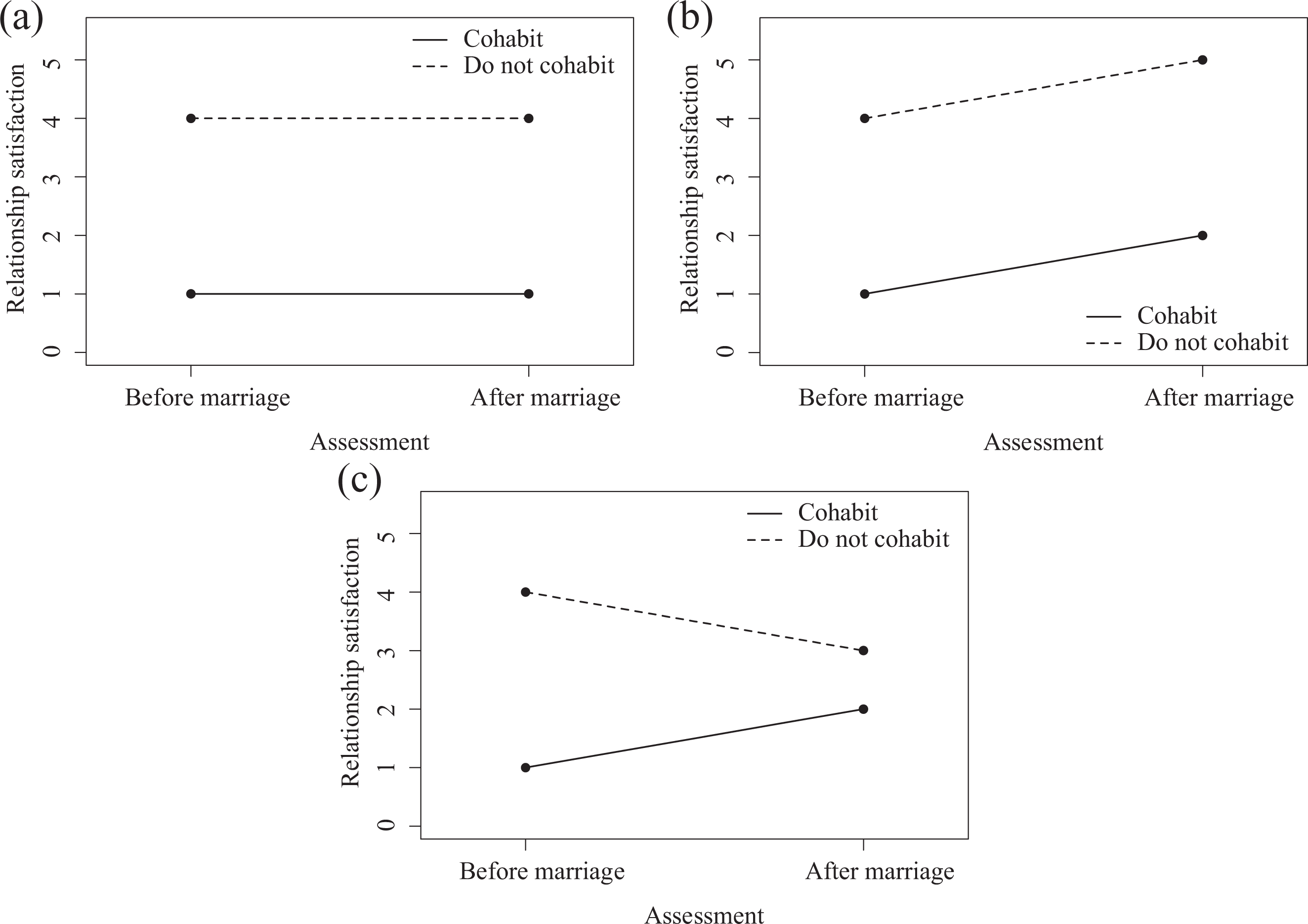
Three possible scenarios of average relationship satisfaction scores across time. (a) No change over time with two populations at baseline. (b) Equal differences in change over time with two populations at baseline. (c) No change over time with one population at baseline.

$R {S_{n}}_{2} = 0 + 1 \times R {S_{n}}_{1} + 0 \times C_{n} + {e_{n}}_{2},$
6

which has the same form as Equation 1. Equation 6 also describes the average patterns in Figure 1b, except that the intercept would equal 1 instead of 0. In sum, the residualized change model (Equation 1) becomes equivalent to the difference score model (Equation 2) when the autoregression coefficient is equal to 1, and this value points to an assumption of the difference score model: Baseline differences on the key predictor will be stable (Figure 1a) or change equally (Figure 1b) across time when there is no effect of the key predictor (i.e., the null hypothesis).

The assumption mentioned earlier is critical to the difference score model and is in contrast to the residualized change approach, for which β₁ in Equation 1 is expected to be less than 1, implying that, when cohabitation has no effect on relationship satisfaction, differences in relationship satisfaction across those who cohabit and those who do not cohabit diminish across time. Figure 1c illustrates this assumption, as the differences across groups in relationship satisfaction after marriage are smaller than before marriage. Indeed, readers can try to use Equation 6 to describe the average relationship satisfaction score after marriage in Figure 1c and will realize this is impossible to do if the autoregressive effect is to remain 1 and the effect of cohabiting is to remain 0. A natural question that might arise at this point is, why would it make sense for differences across groups to diminish across time when there is no effect of the key predictor? The answer lies in the well-known—but not well-understood—statistical artifact: regression toward the mean. This phenomenon entails observing a sample of scores that are closer to the population mean on a second measurement occasion, when extreme scores were sampled from that one population at the first measurement occasion. The key words in the previous statement are “one population” because regression toward the mean would only be expected if and only if the sampled scores at the first measurement occasion belong to the same population. If, however, what one thinks are extreme scores at one measurement occasion are in fact scores that represent two distinct populations, then the mean differences in scores across time should not be expected to change in the absence of an experimental or naturally occurring manipulation.

In our example, the residualized change model assumption is reasonable if scores on relationship satisfaction before marriage were obtained from dyads sampled without bias from one population. One way to find out if this was the case is to look at the correlation of relationship satisfaction before marriage (RS_n1 ) and cohabitation (C_n ), which should tend toward zero as sample size goes to infinity if dyads come from one population with respect to their scores on RS_n ₁.

Recall that coefficients in GLMs are partial regression weights, with the implication that they will vary depending on the correlation between predictors. This is why multicollinearity issues are of concern in regression analysis. When multiple predictors are present, as in Equation 5, their corresponding coefficients will be independent of each other only when the predictors are themselves independent of each other. Otherwise, as correlations across predictors increase, the sensitivity of coefficients to small changes in the predictors also increases. Given this fact, when can we expect relationship satisfaction at Time 1 to be completely uncorrelated with cohabitation? Unfortunately, the only way to assure independence of these two variables is through the use of experimentation procedures. Specifically, we would need to randomly assign couples to cohabit (i.e., an experimental group) or not cohabit (i.e., a control group) prior to marriage and measure their relationship satisfaction before and after marriage. When conducted properly, random assignment guarantees that variability due to dyad’s differences in relationship satisfaction (and all other idiosyncratic dyad’s characteristics) and measurement error is equally distributed across experimental and control groups. However, this is only in infinite samples and with finite samples there is no guarantee that this correlation will be 0 (or near 0).

Clearly, true experiments are not possible for a wide variety of research questions that relationship researchers are interested in answering. Therefore, a nonzero correlation between predictors (e.g., relationship satisfaction prior to marriage and cohabitation) is expected. In the context of our example, the substantive meaning of this correlation is that systematic differences exist in relationship satisfaction prior to marriage (Time 1) across different values of the cohabitation variable. Perhaps those dyads with lower relationship satisfaction are more likely to cohabit prior to marriage (because they are ambivalent about the potential long-term success of the relationship; Jose, O’Leary, & Moyer, 2010) than dyads with higher levels of relationship satisfaction. Alternatively, if we measure cohabitation as a continuous variable, it is possible that dyads with lower relationship satisfaction are more likely to have cohabited for longer periods of time than those with higher relationship satisfaction. These patterns suggest that we are dealing with two different populations, one of cohabitants and another of couples living apart, and each of these has different baseline levels of relationship satisfaction. In sum, when true experimental procedures are not possible or unethical to carry out, it is likely that baseline differences in the outcome exist—there are two populations with respect to the outcome if the key predictor is binary or there are two or more populations with respect to the outcome if the key predictor is continuous—and the residualized change and difference score approaches will yield different conclusions regarding the effect of a key predictor (e.g., cohabiting). Again, this difference in the estimated effect of a key predictor when fitting the ANCOVA and the repeated measures ANOVA models is known as Lord’s paradox.

In closing, we point to the fact that our comparison of models did not require us to make any distributional assumptions of C_n . In other words, our comparison applies equally to cases in which cohabitation (or any key predictor of interest) is a grouping variable or a continuous variable. We portrayed cohabitation as a grouping variable in Figure 1a– for simplicity because the patterns of change are more clearly depicted with a grouping variable.

Empirical comparison of residualized change and difference score models

To illustrate the comparison of the residualized change and difference score models, we simulated two data sets that conform to the motivating example provided in the introductory paragraph. For both data sets, we assumed Sofia collected data on dyad’s relationship satisfaction² 6 months before and after marriage (N = 100), and dyads reported on whether or not they had been cohabiting prior to marriage (C_n = 0 or 1 for negative and affirmative answers, respectively). To facilitate the didactic presentation of this empirical comparison, we simulated data sets with features that are not likely to hold in real life, but in a later example, we incorporate more realistic features into the data and replicate our results. Here, both data sets have an equal number of dyads that did and did not cohabit, and cohabitation had a null effect on changes in relationship satisfaction. Moreover, dyads did not exhibit any changes in relationship satisfaction over time in both data sets. Finally, the only way in which the data sets varied was in the existence of preexisting groups at the premarriage assessment. That is, because in a real investigation of cohabitation a controlled experiment would not be feasible, we generated one data set (i.e., data set A) with lower relationship satisfaction at baseline for dyads who reported cohabiting. The remaining data set (i.e., data set B) did not have this feature—all dyads at the first occasion of assessment came from the same population regardless of whether they cohabited or not. Data set B would only be obtained if Sofia could have randomly assigned dyads to cohabit or live apart. Despite the highly unlikely nature of this data set, we included it here for completeness and to facilitate the comparison of models. R code for generating these data sets is included in the Appendix, and interested readers can change the parameters in the data-generating model to explore corresponding implications. Note that our description of the first dataset corresponds to the assumption made by the difference score model (i.e., no change between groups across time under the assumption of the null hypothesis for the key predictor; there are two populations at baseline), and the second data set is in line with the assumption of the residualized change model, where the Time 1 score is uncorrelated with the key predictor, which is equivalent to affirming there are no preexisting group differences at baseline; there is one population of dyads at baseline with respect to relationship satisfaction.

Table 1 shows descriptive statistics for our mock data sets. These statistics are in line with the aforementioned description of the data sets; aside from measurement error, the baseline levels of relationship satisfaction in data set A differ by about 1 unit (M = 4.46 and 3.44, for no cohabiting and cohabiting respectively). In contrast, data set B has no differences (besides some measurement error) in premarriage relationship satisfaction across groups (M = 4.46 and 4.44, for no cohabiting and cohabiting, respectively). Also, notice that we generated the exact same values across data sets for the no cohabiting group. Thus, the only differences across data sets are in the values for those who reported cohabiting prior to marriage.

Table 1.
Descriptive statistics for two simulated examples differing on the existence of preexisting cohabitation group differences.

Cohabit = 0 (No) Cohabit = 1 (Yes)

Premarriage RS Postmarriage RS Difference RS Premarriage RS Postmarriage RS Difference RS

Data set A. No change but cohabitation group difference in premarriage scores

Mean 4.46 4.54 .08 3.44 3.48 .04

SD .30 .31 .45 .31 .31 .43

Min 3.85 3.68 −.77 2.80 2.64 −1.26

Max 5.12 5.15 .85 4.26 4.41 1.13

n 50 50 50 50 50 50

Data set B. No change and no cohabitation group difference in premarriage scores

Mean 4.46 4.54 .08 4.44 4.48 .04

SD .30 .31 .45 .31 .31 .43

Min 3.85 3.68 −.77 3.80 3.64 −1.26

Max 5.12 5.15 .85 5.26 5.41 1.13

n 50 50 50 50 50 50

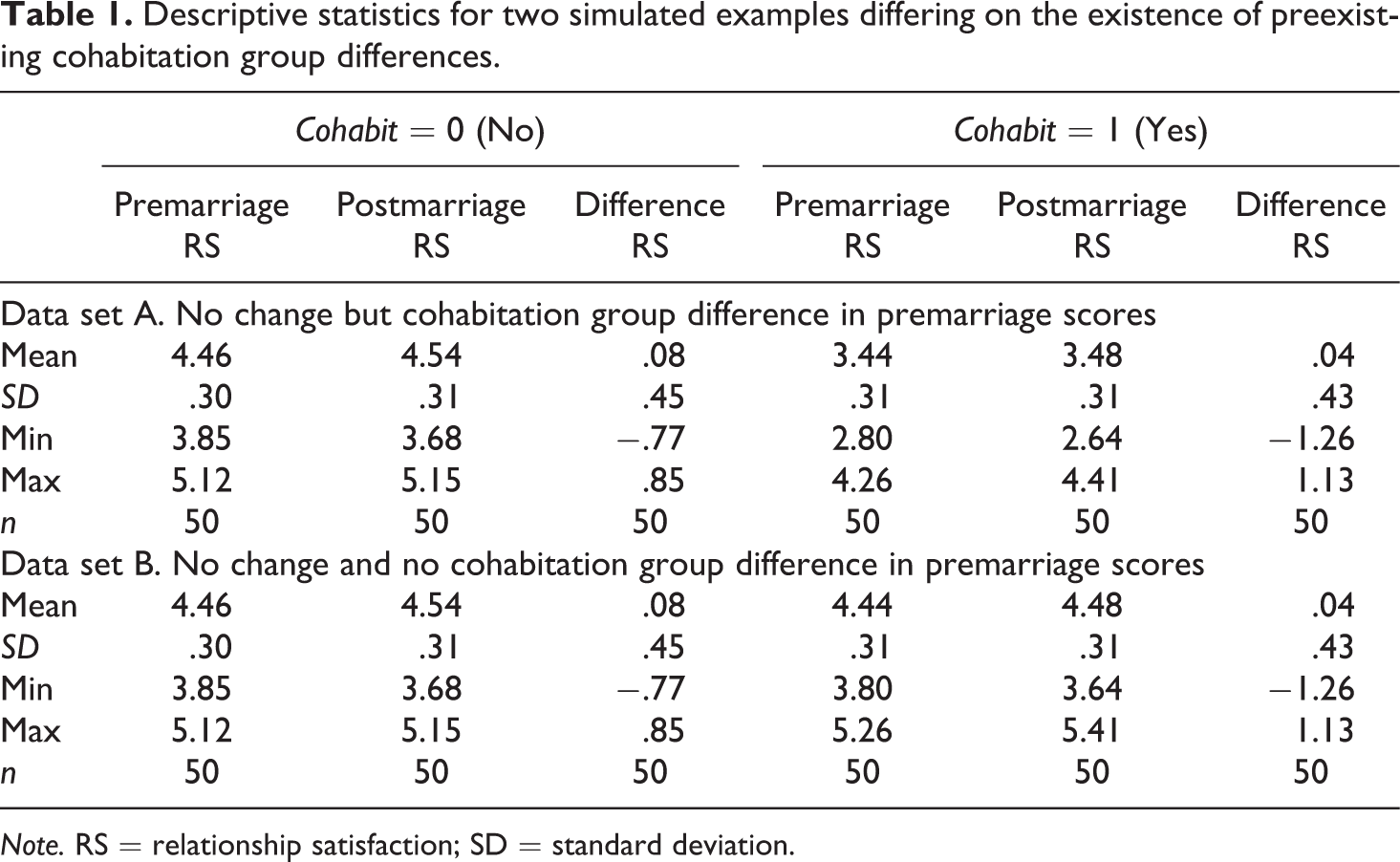
Note. RS = relationship satisfaction; SD = standard deviation.

Figure 2 and Table 2 complement the descriptive statistics of Table 1. Figure 2 contains scatterplots of the association between pre- and postmarriage relationship satisfaction by cohabiting group. Differences in relationship satisfaction at the baseline assessment are obvious in panel A and absent in panel B. Moreover, Table 2 shows the correlation coefficients (with associated p values above the diagonals) across the variables of interest for both data sets. Of key importance is the strong and significant correlation among relationship satisfaction at Time 1 and cohabitation in data set A (r = −.86, p < .01). The equivalent coefficient in data set B is nearly zero (r = −.03, p = .78). As mentioned before, this association is introduced by the existence of preexisting groups at baseline. Cohabitation also has a strong correlation with relationship satisfaction at Time 2 (r = −.86, p ≤ .01) in data set A but that is not the case in data set B (r = −.09, p = .36).

Figure 2.
Scatterplot of simulated data set with (dataset a, panel a) and without (data set b, panel b) preexisting mean differences in relationship satisfaction at Time 1 and no significant change in group mean differences over time. Solid circles represent dyads who did not cohabit prior to marriage. Solid triangles represent dyads who cohabited prior to marriage.

Table 2.
Correlation matrices for two simulated examples differing on the existence of preexisting cohabitation group differences.

1 2 3 4

Data set A. No change but cohabitation group difference in premarriage scores

1. Cohabit 1.00 < .001 < .001 .65

2. Time 1 relationship satisfaction −.86 1.00 < .001 < .001

3. Time 2 relationship satisfaction −.86 .74 1.00 < .001

4. Relationship satisfaction change −.05 −.32 .40 1.00

Data set B. No change and no cohabitation group difference in premarriage scores

1. Cohabit 1.00 .78 .36 .65

2. Time 1 relationship satisfaction −.03 1.00 .80 < .001

3. Time 2 relationship satisfaction −.09 −.03 1.00 < .001

4. Relationship satisfaction change −.05 −.71 .73 1.00

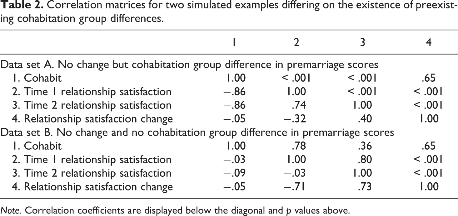
Note. Correlation coefficients are displayed below the diagonal and p values above.

We fit the residualized and difference score models to each of our data sets, and the results are summarized in Table 3. Recall that the main interest in these analyses is to assess the potential effect of cohabitation on changes in relationship satisfaction. According to the residualized change model we fit to data set A (which is an ANCOVA model in this application because of the categorical predictor), the factors explain 75% of the variance in the outcome, F(2, 97) = 144.00, p < .01, R ² = .75, and results suggest there is a statistically and practically significant effect of cohabitation in dyad’s relationship satisfaction at Time 2 while controlling for baseline relationship satisfaction, b = −1.09, SE = .12, t = −8.86, p < .01. In contrast, when we fit the difference score model to the same data, less than 1% of the variance in the outcome is explained by the model, F(1, 98) = .21, p = .65, R ² = .002, and results suggested that cohabitation did not have an effect on relationship satisfaction change, b = −.04, SE = .09, t = −.46, p = .65. As expected, the inferences from these models are strikingly different, which is an example of Lord’s paradox and can be attributed to the differences in baseline scores across couples who cohabit and those who do not.

Table 3.
Coefficients from fitting the residualized change and difference score models to simulated data sets A and B, which exhibit no change over time but differ in baseline levels of a grouping variable.

Predictor Estimate SE t p

Data set A

Residualized Change Model

Intercept 4.67 .47 10.03 < .001

Time 1 relationship satisfaction −.03 .10 −.28 .78

Cohabit −1.09 .12 −8.86 < .001

Difference score model

Intercept .08 .06 1.28 .20

Cohabit −.04 .09 −.46 .65

Dataset B

Residualized change model

Intercept 4.67 .47 10.03 < .001

Time 1 relationship satisfaction −.03 .10 −.28 .78

Cohabit −.06 .06 −.92 .36

Difference score model

Intercept .08 .06 1.28 .20

Cohabit −.04 .09 −.46 .65

Results from fitting the residualized change model to data set B suggested that the factors did not explain significant variability in the outcome, F(2, 97) = .45, p = .64, R ² = .009. Specifically, results pointed to a lack of effect of cohabitation on relationship satisfaction while accounting for baseline levels of the outcome, b = −.06, SE = .06, t = −.92, p = .36. And a similar null effect of cohabitation emerged from fitting the difference score model to this data set, b = −.04, SE = .08, t = −.46, p = .65. Because the difference score model only has one predictor, the F ratio for the model is the latter t value squared, F(1, 98) = .21, p = .65, and the variance explained by the model is near zero, R ² = .002. Thus, the difference score model leads us to the correct inferences in both datasets, and the residualized change model is biased when preexisting differences in cohabitation exist at baseline (data set A).

Results from the models above emphasize the differences between the residualized change and difference score models. Because there is no change across groups over time in either data set, the difference score model guided us toward the correct inference (of lack of cohabiting effect) in both of the applications. On the other hand, the residualized change model leads us to the wrong inference (of significant cohabiting effect) when the data exhibit baseline differences across groups. But when the latter is not the case, as in data set B, the residualized change model performs appropriately and is in fact more accurate and powerful than the difference score model. The improved power of the residualized change model when used under appropriate conditions is exemplified by the smaller standard error of the key predictor’s effect (SE = .06 versus .09 for the difference score model; see Table 3) and is due to the autoregressive effect accounting for variation in the outcome, which makes the residual variance smaller in this model (for further details see van Breukelen, 2013).

To wrap up our comparison of models, we confirmed—empirically—two assertions made in the previous section. First, the residualized change model with postmarriage scores as the outcome (as in Equation 1) is perfectly equivalent to using the difference score as the outcome and controlling for baseline differences (as in Equation 5); and second, it is not required to make distributional assumptions of the key predictor, C_n , for our statements to hold when comparing the two models. To illustrate the former assertion, we fit the model in Equation 5 to data sets A and B. In both instances, all parameter estimates and standard errors were identical to those displayed in Table 3 for the residualized change model, with the exception of one: As expected, the regression coefficient for relationship satisfaction at Time 2 on Time 1 was −1.03 (SE = .10, p < .01) for both data sets, which is equal to −.03 − 1 (β₁ – 1).

Moreover, we confirmed our second assertion by simulating two additional example data sets (i.e., C and D) with a few differences from the previous data sets. Namely, we included a cohabitation variable that is continuous (rather than categorical) and represents the time in months that couples have lived together prior to marriage. Data sets C and D are also more realistic (compared to A and B) because we set up relationship satisfaction over time to be positively correlated, and the mean of relationship satisfaction after marriage is slightly lower than the mean of relationship satisfaction prior to marriage. These features are in line with the literature on cohabitation and relationship satisfaction (Jose et al., 2010). To provide an additional resource for readers, we simulated these data sets using M plus version 7 (Muthén & Muthén, 1998-2012) and provide the code in the Appendix for those interested in replicating the analysis. The population parameters for simulating the data set are somewhat different from the previous example, yet the key characteristic remains: There is no effect of cohabitation on relationship satisfaction change over time, but there is a correlation of cohabitation with relationship satisfaction at baseline in data set C, and this correlation is null in data set D.

Descriptive statistics and correlation coefficients for variables in data sets C and D are included in Table 4. The pattern of correlations is very similar to that in Table 2. That is, cohabitation and relationship satisfaction at time 1 are significantly correlated in data set C (r = −.53, p < .001) but not in data set D (r = −.04, p = .73), pointing to baseline differences that depend on the key predictor. Moreover, the average relationship satisfaction at time 2 (M = 4.51) is lower than at time 1 (M = 5.08) in both data sets. Table 5 includes results from fitting the alternative models to data sets C and D. Fitting the residualized change model to data set C resulted in a significant negative effect of cohabitation (b = −.31, SE = .03, t = −9.09, p < .001) on relationship satisfaction after marriage while controlling for premarriage levels of relationship satisfaction. Using the exact same data set but fitting the difference score model produced the correct inference; the effect of cohabiting on relationship satisfaction differences was null (b = −.001, SE = .06, t = -.01, p = .99). As with data set B, fitting the residualized change model to data set D resulted in a null effect for cohabitation (b = −.01, SE = .04, t = −.33, p = .74), and this was also the case when the difference score model was fit to data set D (b = .002, SE = .06, t = .04, p = .97). Thus, findings with data sets C and D replicate our findings with data sets A and B but with more realistic features in the data and with a continuous predictor.

Table 4.
Correlation matrices, means, and SD for two simulated examples differing on the existence of preexisting group differences.

1 2 3 4 M SD

Data set C. No effect of cohabitation on change but preexisting groups in premarriage scores

1. Cohabit 1.00 < .001 < .001 .99 11.99 .98

2. Time 1 relationship satisfaction −.53 1.00 < .001 < .001 5.08 1.01

3. Time 2 relationship satisfaction −.75 .85 1.00 .01 4.51 .71

4. Relationship satisfaction change .00 −.73 −.26 1.00 −.56 .56

Dataset D. No effect of cohabitation on change and no preexisting groups in premarriage scores

1. Cohabit 1.00 .73 .64 .97 11.97 .91

2. Time 1 relationship satisfaction −.04 1.00 < .001 < .001 5.08 1.01

3. Time 2 relationship satisfaction −.05 .85 1.00 .01 4.51 .71

4. Relationship satisfaction change .00 −.73 −.26 1.00 −.56 .56

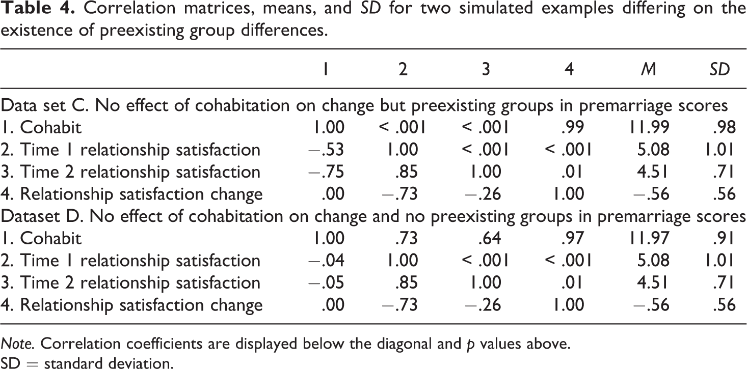
Note. Correlation coefficients are displayed below the diagonal and p values above.

SD = standard deviation.

Table 5.
Coefficients from fitting the residualized change and difference score models to simulated data sets C and D, which exhibit no effect of cohabitation on change over time but differ in baseline levels of a key predictor.

Predictor Estimate SE t p

Data set C

Residualized change model

Intercept 5.95 .51 11.66 < .001

Time 1 relationship satisfaction .44 .03 13.38 < .001

Cohabit −.31 .03 −9.09 < .001

Difference score model

Intercept −.59 .74 −.80 .43

Cohabit .002 .06 .04 .97

Data set D

Residualized change model

Intercept 1.67 .54 3.07 .002

Time 1 relationship satisfaction .59 .04 15.80 < .001

Cohabit −.01 .04 −.33 .74

Difference score model

Intercept −.59 .74 −.80 .43

Cohabit .002 .06 .04 .97

Note. SE = standard error.

Results with data sets C and D are very important because Lord’s paradox has been discussed mostly in the context of a binary key predictor that distinguishes control and treatment groups, yet the paradox and issues associated with it are equally relevant to instances where the key predictor is continuous. In our analyses, the difference score model always arrived at the correct inference, yet the residualized change model only provided the correct inference when baseline levels of relationship satisfaction were uncorrelated with cohabitation (data sets B and D).

Selecting the “correct” model

As we showed above, the residualized change and difference score models will often lead to different inferences about the effect of the predictor of interest. In the examples, we presented the null hypothesis was true in the population. However, even when the null hypothesis is not true in the population (e.g., when there is an effect of cohabitation on dyad’s changes in relationship satisfaction), discrepancies in inferences are still expected. Further illustration of this fact is available in the Appendix, where we include plots and analyses of multiple simulated data sets with alternative patterns of change than those discussed thus far.³

Naturally, a central issue is figuring out which of these two models is most appropriate in a given application. Yet, as others have emphasized before (e.g., Gollwitzer et al., 2014; van Breukelen, 2013; Wainer, 1991), the assumptions each of these models make are untestable, and this makes it challenging to argue that either model is more appropriate than the other. Using our guiding example to clarify further, note that dyads who report cohabiting prior to marriage will never be able to report what their relationship satisfaction after marriage would have been if they had not cohabited. The opposite problem is also true; we will never know what level of relationship satisfaction would have been reported by dyads who did not cohabit before marriage if they had in fact chosen to live with their partners prior to getting married. This is the problem that makes us question the validity of our inferences from either model (see also Wainer, 1991).

One thing we do know, however, is that when experimentation procedures are followed, dyads (or individuals) would be randomly assigned to a grouping variable (the key predictor of interest), and this would lead to the independence of the grouping variable with the pre-test scores. Naturally, because samples are finite, the correlation of grouping variable and pretests scores will not be exactly zero but should be near zero. Thus, proper experimentation prohibits preexisting groups to be formed at baseline. Under such circumstances, the residualized change model and difference score models will arrive at the same inference, but the former has the advantage of having more power because it makes the correct assumption about the distribution of baseline scores.

Which should be our choice when experimentation is not possible? We hope our discussion thus far has clarified that, if we have different populations with different levels of the outcome at baseline, the residualized change model is not appropriate because it will necessarily be biased. We believe the difference score model is a better choice in nonrandomized studies. But naturally, we are never able to observe cohabitants under a no cohabiting condition, and thus, we cannot be certain about cohabitants’ pattern of change under the null hypothesis. We argue that theory, previous investigations, and preliminary analyses can help researchers figure out which assumptions are more tenable. Theory and previous findings might suggest that cohabitants have higher levels of relationship satisfaction in general and perhaps belong to a different population than those dyads who live apart. Also, preliminary analyses can complement these suspicions if statistical and practical significance is found between cohabitation and relationship satisfaction before marriage, which is very likely the case. In sum, we believe the assumption of the difference score model is more tenable and thus, this model has a chance to guide us in the correct direction when analyzing observational data.

As indicated in a previous section, one important issue that has led researchers to stray from fitting the difference score model, despite the fact that it might be most appropriate, is the negative reputation of difference scores from several decades ago. Thus, as difference scores fell out of favor, researchers opted to fit the residualized change model. But advances in methodology now allow us to model latent difference (or change) scores that are error-free. Before describing these models, however, we discuss the role of measurement error in the residualized change and difference score models.

Measurement error

Measurement error in observed variables led to a great deal of disparagement of difference scores. So a fair question to ask is, how does measurement error and potentially low reliability of difference scores influence our choice between the residualized change and difference score models? The short answer is, it does not.

We know measurement error is present in our data, whether differenced or not. Thus, we must understand the implications and important distinctions of having measurement error in predictor and outcome variables of a GLM. We know that as measurement error in predictor variables increases, downward bias in the regression coefficients of the model in Equations 1 through 5 increases. On the other hand, when the outcome variable has high measurement error, the residual term in Equations 1 through 5 will increase and, as a result, we lose precision in the point estimates of the model.

Focusing on Equation 2, it is likely that the difference score in the outcome has a significant amount of measurement error; this would decrease the power of our test to find a significant effect of cohabitation. At the same time, measurement error in our cohabitation measure will attenuate the effect of cohabitation. The corresponding loss of power and amount of attenuation is related to the amount of measurement error in the variables involved. In other words, measurement error obscures the true relations between variables of interest, making our already difficult task more challenging. At times, measurement error is responsible for encountering Lord’s paradox (Gollwitzer et al., 2014).

The specification of latent variables in SEM undoubtedly presents advantages to relationship researchers and all social scientists alike. On the one hand, latent variables allow us to capture and model error-free constructs, and on the other hand, modern missing data techniques can be implemented with ease in this framework, maximizing our sample size and thus our power to detect effects. Importantly, van Breukelen (2013) showed that using SEM to correct for measurement error in the outcome and predictor(s) of latent residualized change or latent difference score models, does not change the repercussions of having preexisting groups (or correlated baseline with key predictor) in the first measurement occasion. Thus, in nonrandomized studies, a latent difference score model should still be preferred over a latent residualized change model.

Latent change score framework

McArdle and Nesselroade (1994) were the first to show how to specify a latent change, or difference, variable in SEM (see Figure 3a for the specification in the context of our example). The specification relies on the same notions we discussed when comparing the residualized change and difference score models. That is, one can specify a regression of the Time 2 outcome on the baseline level of the outcome and fix the prediction to 1. This perfect prediction transforms the meaning of the residual of the regression into a latent change, or difference, variable. Moreover, because the regression coefficient was not freely estimated, it is possible to estimate the covariance of the baseline score with the change score (σ_RS1,Δ in Figure 3a). One can also estimate a mean for the baseline score and the change score (μ_RS1 and μ_Δ , respectively, in Figure 3a), by regressing the corresponding variables on a constant; the constant is depicted by a triangle in Figure 3a. The model implied by the path diagram in Figure 3a can be extended to include the effect of a key predictor (e.g., cohabitation) on the LCS; such model is shown in Figure 3b. Notice the path diagram in Figure 3b implies the following equation for the change in relationship satisfaction,

Figure 3.
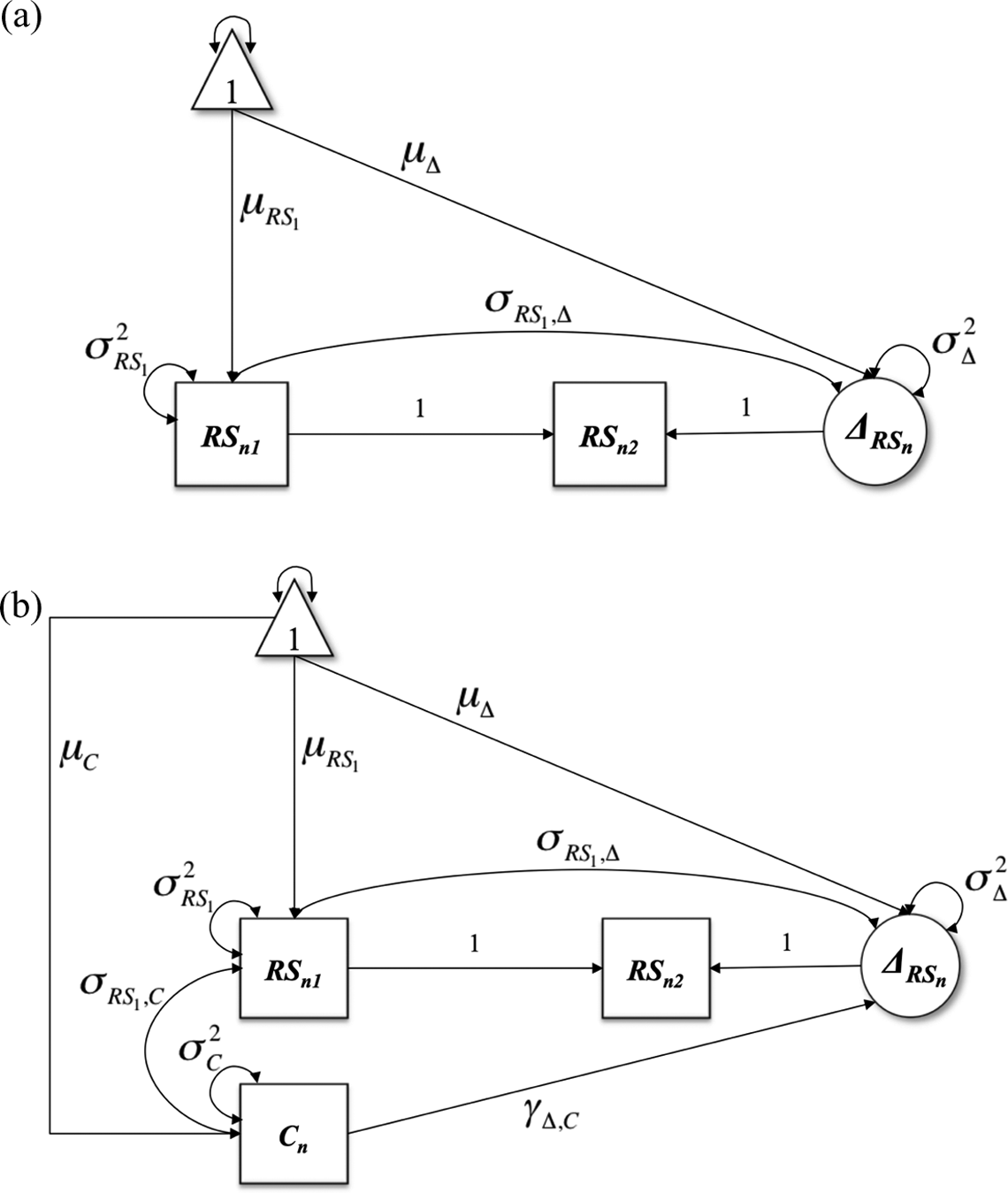
(a) Path diagram of latent change score specification for relationship satisfaction. (b) Path diagram of the difference score model in Equation 2. Squares represent manifest variables, circles are latent variables, and the triangle is a constant for estimating means.

$Δ R S_{n} = μ_{Δ} + γ_{Δ, C} C_{n} + {σ^{2}}_{Δ n,}$
7

where ΔRS_n is the change, or difference, between pre- and postmarriage relationship satisfaction, RS_n2 − RS_n1 , μ_Δ is an intercept equal to γ₀ in Equation 2, γ_{Δ, C} is a regression coefficient equal to γ₁ in Equation 2, and σ² _Δn is a residual equal to e_n(RS _2−RS1) in Equation 2. Thus, despite the different notation traditionally used in SEM, the model in Figure 3b is exactly the same model as the difference score model in Equation 2. Notably, although ΔRS_n in Figure 3a and 3B is a latent variable, the variable is not purged of measurement error.

To take full advantage of the SEM framework, the models in panels A and B of Figure 3 should be augmented to include latent variables for relationship satisfaction before and after marriage. Specifying latent variables with multiple indicators of relationship satisfaction would allow us to model error-free (i.e., perfectly reliable) variables and, importantly, the LCS variable would also be error free. To emphasize the latter point further, let us revisit Lord’s assertion,
If psychological tests were perfectly reliable, there would be no need for further discussion, since the best estimate of a pupil’s gain would be obtained by the obvious procedure of subtracting his [sic] score on the first test from his score on the second. (Lord, 1956, p. 421)
Indeed, there is no need for further discussion. A critical advantage of LCS models with multiple indicators is that the criticisms that once thwarted the use of difference scores become moot (for an example of an application of these models with two occasions of data, including Mplus code, see Henk & Castro-Schilo, 2016). Importantly, when multiple indicator latent variables are included in a model, such as that in Figure 3b, researchers must perform preliminary analyses to test for factorial invariance of the construct over time. Widaman and Reise (1997) provide guidelines for how to perform these tests. Briefly, strong factorial invariance is required to ascertain that the same construct has been measured over time in the same scale and for the associated latent change variables to be meaningful.

If the model in Figure 3a had latent variables for relationship satisfaction, then this model could be described as a measurement model that permits explicit modeling of error-free changes. This measurement model gives us tremendous flexibility for modeling change in a variety of ways. For example, one of the best-known LCS models introduced by McArdle and colleagues (McArdle, 2001; McArdle & Hamagami, 2001) is referred to as the dual LCS model. In this model, McArdle and colleagues posit the latent changes as emerging from two sources: a proportion of the status of the variable at the previous time point and a developmental factor that can be constant or not constant over time. Other LCS models have surfaced in the last few years, such as those that can directly capture not only rates of change but also acceleration (Grimm, Zhang, Hamagami, & Mazzocco, 2013), those that allow latent changes to be predictors and outcomes (Grimm, An, McArdle, Zonderman, & Resnick, 2012; Henk & Castro-Schilo, 2016), others that permit modeling of nonlinear trajectories (Grimm, Castro-Schilo, & Davoudzadeh, 2013; Grimm et al., 2012), and those that explore preliminary mediation processes with two-occasion data (Henk & Castro-Schilo, 2016). Of particular interest to relationship researchers, Lida, Seidman, and Shrouth (2017), is discussing the possibility of using the LCS framework when fitting the dyadic score model. Indeed, the flexibility afforded by the explicit representation of latent changes in SEM makes traditional difference models (e.g., repeated measures ANOVA and t test) estimable in SEM but with the added benefit of having error-free difference variables. Naturally, with increased flexibility comes added responsibility. The flexibility of a LCS framework suggests researchers must consider carefully their hypothesis about change and how it should be structured.

Although outside the scope of this article, it is worth noting that with more than two occasions of data, researchers often rely on latent growth curve (LGC) models for the analysis of change (McArdle & Epstein, 1987; Meredith & Tisak, 1990). The LGC models can be specified in the LCS framework (see Grimm et al., 2013 for details) and, thus, are a more complex and elegant type of difference score model. Specifically, LGC models include the specification of an LCS (the slope) that is based on the, often linear, rate of change estimated over a series of repeated measures. Note that no variables are residualized to attain the specification of the slope, or LCS.

Summary

As in other fields in psychology, close relationship researchers are often concerned with data that span two occasions and where the effect of a key predictor in the change across time is central to a research question. In our guiding example, Sofia was interested in studying change in relationship satisfaction among couples who did or did not cohabit prior to marriage. She recognized two statistical models for testing her hypothesis and wondered which of these techniques is most appropriate for her application? Should both strategies provide the same results? Why do difference scores have a bad reputation? Are there additional strategies that might be preferred over her current options?

If Sofia were to approach us today with these inquiries, our answers would be as follows. The observational nature of her data and the intuitive expectation that dyads with low relationship satisfaction self-select to cohabit prior to marriage suggest that a difference score model should be employed. We would advise our fictional character to estimate the correlation between baseline relationship satisfaction and cohabitation, in addition to estimating the means of relationship satisfaction before marriage for each cohabiting group to assess the degree of baseline differences in the construct. Moreover, we would remind Sofia that the assumption of the difference score model might not be tenable, but unfortunately we cannot test it because we are unable to observe cohabiting couples under a no cohabiting condition. We would also remind her that an ANCOVA model makes the assumption that no baseline differences across cohabiting groups exist, and thus, fitting an ANCOVA model might lead her to the wrong conclusion. In our imaginary consulting session, we would emphasize that our advice applies equally to the problem at hand irrespective of having a grouping or continuous variable for cohabitation.

Having heard rumors about the low reliability of difference scores, Sofia might push back and feel hesitant to adopt a difference score model. We would assure her, however, that a paired t-test is a difference score model as is repeated measures ANOVA and a LGC with two time points,⁴ all of which are widely used and accepted under the appropriate context. Moreover, we would strongly argue for her to consider using SEM for fitting the difference score model but with latent relationship satisfaction variables. As a result, she would be able to model an error-free latent change variable that has perfect reliability, and would be able to use full information maximum likelihood to account for any missing data in her sample, assuming the data are missing at random.

In sum, with current advances in methodology, especially with LCS models with multiple indicators, there is little room (if any) for residualized change approaches in nonrandomized studies. As Sofia’s consultants, we would make sure she knows this and shares it with as many colleagues as possible.

	Cohabit = 0 (No)	Cohabit = 1 (Yes)
Data set A. No change but cohabitation group difference in premarriage scores
Mean	4.46	4.54	.08	3.44	3.48	.04
SD	.30	.31	.45	.31	.31	.43
Min	3.85	3.68	−.77	2.80	2.64	−1.26
Max	5.12	5.15	.85	4.26	4.41	1.13
n	50	50	50	50	50	50
Data set B. No change and no cohabitation group difference in premarriage scores
Mean	4.46	4.54	.08	4.44	4.48	.04
SD	.30	.31	.45	.31	.31	.43
Min	3.85	3.68	−.77	3.80	3.64	−1.26
Max	5.12	5.15	.85	5.26	5.41	1.13
n	50	50	50	50	50	50

	1	2	3	4
Data set A. No change but cohabitation group difference in premarriage scores
1. Cohabit	1.00	< .001	< .001	.65
2. Time 1 relationship satisfaction	−.86	1.00	< .001	< .001
3. Time 2 relationship satisfaction	−.86	.74	1.00	< .001
4. Relationship satisfaction change	−.05	−.32	.40	1.00
Data set B. No change and no cohabitation group difference in premarriage scores
1. Cohabit	1.00	.78	.36	.65
2. Time 1 relationship satisfaction	−.03	1.00	.80	< .001
3. Time 2 relationship satisfaction	−.09	−.03	1.00	< .001
4. Relationship satisfaction change	−.05	−.71	.73	1.00

Predictor	Estimate	SE	t	p
Data set A
Residualized Change Model
Intercept	4.67	.47	10.03	< .001
Time 1 relationship satisfaction	−.03	.10	−.28	.78
Cohabit	−1.09	.12	−8.86	< .001
Difference score model
Intercept	.08	.06	1.28	.20
Cohabit	−.04	.09	−.46	.65
Dataset B
Residualized change model
Intercept	4.67	.47	10.03	< .001
Time 1 relationship satisfaction	−.03	.10	−.28	.78
Cohabit	−.06	.06	−.92	.36
Difference score model
Intercept	.08	.06	1.28	.20
Cohabit	−.04	.09	−.46	.65

	1	2	3	4	M	SD
Data set C. No effect of cohabitation on change but preexisting groups in premarriage scores
1. Cohabit	1.00	< .001	< .001	.99	11.99	.98
2. Time 1 relationship satisfaction	−.53	1.00	< .001	< .001	5.08	1.01
3. Time 2 relationship satisfaction	−.75	.85	1.00	.01	4.51	.71
4. Relationship satisfaction change	.00	−.73	−.26	1.00	−.56	.56
Dataset D. No effect of cohabitation on change and no preexisting groups in premarriage scores
1. Cohabit	1.00	.73	.64	.97	11.97	.91
2. Time 1 relationship satisfaction	−.04	1.00	< .001	< .001	5.08	1.01
3. Time 2 relationship satisfaction	−.05	.85	1.00	.01	4.51	.71
4. Relationship satisfaction change	.00	−.73	−.26	1.00	−.56	.56

Predictor	Estimate	SE	t	p
Data set C
Residualized change model
Intercept	5.95	.51	11.66	< .001
Time 1 relationship satisfaction	.44	.03	13.38	< .001
Cohabit	−.31	.03	−9.09	< .001
Difference score model
Intercept	−.59	.74	−.80	.43
Cohabit	.002	.06	.04	.97
Data set D
Residualized change model
Intercept	1.67	.54	3.07	.002
Time 1 relationship satisfaction	.59	.04	15.80	< .001
Cohabit	−.01	.04	−.33	.74
Difference score model
Intercept	−.59	.74	−.80	.43
Cohabit	.002	.06	.04	.97

Footnotes

Funding

The author(s) disclosed receipt of the following financial support for the research, authorship, and/or publication of this article: Kevin J. Grimm was supported by National Science Foundation Grant REAL–1252463 awarded to the University of Virginia, David Grissmer (Principal Investigator), and Christopher Hulleman (Co-Principal Investigator).

ORCID iD

Kevin J. Grimm

Notes

Appendix

References

Cronbach

L. J.

Furby

(1970). How should we measure “change”—or should we? Psychological Bulletin, 74, 68–80.

Eriksson

Häggström

(2014). Lord’s paradox in a continuous setting and a regression artifact in numerical cognition research. Plos One, 9, 1–7.

Gollwitzer

Christ

Lemmer

(2014). Individual differences make a difference: On the use and the psychometric properties of difference scores in social psychology. European Journal of Social Psychology, 44, 673–682.

Gottman

J. M.

Rushe

R. H.

(1993). The analysis of change: Issues, fallacies, and new ideas. Journal of Consulting and Clinical Psychology, 61, 907–910.

Grimm

K. J.

McArdle

J. J.

Zonderman

A. B.

Resnick

S. M.

(2012). Recent changes leading to subsequent changes: Extensions of multivariate latent difference score models. Structural Equation Modeling: A Multidisciplinary Journal, 19, 268–292.

Grimm

K. J.

Casto-Schilo

Davoudzadeh

(2013). Modeling intraindividual change in nonlinear growth models with latent change scores. GeroPsych, 26, 153–162.

Grimm

K. J.

Zhang

Hamagami

Mazzocco

M. M.

(2013). Modeling nonlinear change via latent change and latent acceleration frameworks: Examining velocity and acceleration of growth trajectories. Multivariate Behavioral Research, 48, 117–143.

Henk

C. M.

Castro-Schilo

(2016). Preliminary detection of relations among dynamic processes with two-occasion data. Structural Equation Modeling, 23, 180–193.

Jose

O’Leary

K. D.

Moyer

(2010). Does premarital cohabitation predict subsequent marital stability and marital quality? A meta-analysis. Journal of Marriage and Family, 72, 105–116.

10.

Lida

Seidman

Shrout

P. E

. (2017). Models of interdependent individuals and dyadic process in relationship research. Journal of Social and Personal Relationships.

11.

Liker

J. K.

Augustyniak

Duncan

G. J.

(1985). Panel data and models of change: A comparison of first difference and conventional two-wave models. Social Science Research, 14, 80–101.

12.

Lord

F. M.

(1956). The measurement of growth. Educational and Psychological Measurement, 16, 421–437.

13.

Lord

F. M.

(1967). A paradox in the interpretation of group comparisons. Psychological Bulletin, 68, 304–305.

14.

Maris

(1998). Covariance adjustment versus gain scores revisited. Psychological Methods, 3, 309–327.

15.

McArdle

J. J.

(2001). A latent difference score approach to longitudinal dynamic structural analysis. In Cudeck

du Toit

Sörbom

(Eds.), Structural equation modeling: Present and future. A Festschrift in honor of Karl Jöreskog (pp. 341–380). Lincolnwood, IL: Scientific Software International.

16.

McArdle

J. J.

Epstein

(1987). Latent growth curves within developmental structural equation models. Child Development, 58, 110–133.

17.

McArdle

J. J.

Hamagami

(2001). Latent difference score structural models for linear dynamic analyses with incomplete longitudinal data. In Collins

L. M.

Sayer

A. G.

(Eds.), New methods for the analysis of change (pp. 137–176). Washington, DC: American Psychological Association. doi:10.1037/10409-005

18.

McArdle

J. J.

Nesselroade

J. R.

(1994). Using multivariate data to structure developmental change. In Cohen

S. H.

Reese

H. W.

(Eds.), Life-span developmental psychology: Methodological innovations (pp. 223–267). Hillsdale, NJ: Erlbaum.

19.

Meredith

Tisak

(1990). Latent curve analysis. Psychometrika, 55, 107–122.

20.

Muthén

L. K.

Muthén

B. O

. (1998–2012). User’s guide (7th ed.). Los Angeles, CA: Muthén & Muthén.

21.

Pearl

(2014, 10 3). Lord’s paradox revisited – (Oh Lord! Kumbaya!). Technical Report. Retrieved from http://ftp.cs.ucla.edu/pub/stat_ser/r436.pdf

22.

Rogosa

Brandt

Zimowski

(1982). A growth curve approach to the measurement of change. Psychological Bulletin, 92, 726–748.

23.

Rogosa

D. W.

Willett

J. B.

(1983). Demonstrating the reliability of the difference score in the measurement of change. Journal of Education Measurement, 20, 335–343.

24.

van Breukelen

G. J. P.

(2013). ANCOVA versus CHANGE from baseline in nonrandomized studies: The difference. Multivariate Behavioral Research, 48, 895–922.

25.

Wainer

(1991). Adjusting for differential base rates: Lord’s paradox again. Psychological Bulletin, 109, 147–151.

26.

Widaman

K. F.

Reise

S. P.

(1997). Exploring the measurement invariance of psychological instruments: Applications in the substance use domain. In Bryant

K. J.

Windle

West

S. G.

(Eds.), The science of prevention: Methodological advances from alcohol and substance use research (pp. 281–324). Washington, DC: American Psychological Association. doi:10.1037/10222-009

	Cohabit = 0 (No)			Cohabit = 1 (Yes)
	Premarriage RS	Postmarriage RS	Difference RS	Premarriage RS	Postmarriage RS	Difference RS
Data set A. No change but cohabitation group difference in premarriage scores
Mean	4.46	4.54	.08	3.44	3.48	.04
SD	.30	.31	.45	.31	.31	.43
Min	3.85	3.68	−.77	2.80	2.64	−1.26
Max	5.12	5.15	.85	4.26	4.41	1.13
n	50	50	50	50	50	50
Data set B. No change and no cohabitation group difference in premarriage scores
Mean	4.46	4.54	.08	4.44	4.48	.04
SD	.30	.31	.45	.31	.31	.43
Min	3.85	3.68	−.77	3.80	3.64	−1.26
Max	5.12	5.15	.85	5.26	5.41	1.13
n	50	50	50	50	50	50