Modeling the consequences of the transition to parenthood: Applications of panel regression methods

Abstract

The transition to parenthood is a topic of substantial interest to family researchers across the social sciences, and many theoretical paradigms have been invoked to understand how it affects men’s and women’s lives. While early empirical scholarship on the transition to parenthood relied on cross-sectional data and methods, the increasing availability of panel data has opened up new analytical pathways—including the possibility to track the same individuals over time as they approach and experience parenthood and their children grow older. By making full use of longitudinal data, researchers can both improve estimation of the consequences of parenthood, as well as advance knowledge by testing more nuanced and complex theoretical premises involving time dynamics. In this article, I present an overview of panel regression models, a family of specifications that can be leveraged for these purposes. In doing so, I discuss the data requirements, advantages and disadvantages of different models, pointing to useful examples of published research. The approaches considered include random effects and fixed effects panel regression models, specifications to model linear and nonlinear time dynamics, and specifications to handle dyadic data structures. The use of these techniques is exemplified via an application considering the effect of motherhood on time pressure using long-running panel data from an Australian national sample, the Household, Income and Labour Dynamics in Australia Survey (n = 68,911 observations; 10,734 women).

Keywords

Change over time dyadic data life course panel data parenthood transition

For a long time, social scientists have been fascinated with the transition to parenthood, with a wealth of scholarship from sociology, psychology, demography, or economics focusing on how becoming a parent is associated with immediate as well as long-term changes in individuals’ personal, family, and work lives (Nomaguchi & Milkie, 2003; Rossi, 1968). Many theoretical paradigms have been used to understand the transition to parenthood and its effect on individuals’ lives. In life-course theory (Elder, Johnson, & Crosnoe, 2003), becoming a parent constitutes a key life-course transition, a critical or sensitive period which has the capacity to shift individuals’ life trajectories across life domains. In the stress process model (Pearlin, 2009), parenthood contributes to the emergence of new stressors that lead onto stress manifestations, as well as the depletion of coping resources. In family systems theory (Minuchin, 1988), the addition of a child to the couple dyad adds complexity to the family system, with the emergence of subsystems and the potential for destabilization.

Following these and other theoretical perspectives, empirical studies have documented that the transition to parenthood has transformational effects on individuals’ lives (Nomaguchi & Milkie, 2003). It is associated with reduced leisure time (Claxton & Perry-Jenkins, 2008), physical activity (Perales, del Pozo-Cruz, & del Pozo-Cruz, 2015), and sleep (Plage, Perales, & Baxter, 2016), complex changes in gender-role attitudes (Baxter, Buchler, Perales, & Western, 2015), shifts in employment status and hours (Hynes & Clarkberg, 2005), worsening physical and mental health (Hewitt, Baxter, & Western, 2006; Nomaguchi & Milkie, 2003), and lower relationship quality (Delicate, Ayers, & McMullen, 2018), to name just a few. Because of gendered normative expectations of mothers as caregivers and insufficient institutional support to parents, the transition to parenthood is often found to have more deleterious effects on women’s than men’s outcomes—triggering or intensifying gender inequalities at home and at work (Baxter, Hewitt, & Haynes, 2008).

The breadth of existing social science scholarship on the transition to parenthood has relied on different methodological approaches to understand the consequences associated with becoming a parent. Early scholarship relied on cross-sectional survey data sets, and so basic cross-sectional modeling approaches were deployed (e.g., ordinary least squares or logistic regression). The increasing availability of panel data from longitudinal surveys opened up new analytical pathways, including the possibility to track the same individuals over time as they approach and experience parenthood and their children grow older.

In this article, I review common and emerging panel regression methods used in previous research concerned with the transition to parenthood. In doing so, I discuss the data requirements, advantages and disadvantages of each approach, and point to useful examples of published research. Although this manuscript assumes some level of statistical competence on the part of the reader, the aim is not to provide a thorough statistical account of the mathematical properties of different estimators. Instead, the goal is to offer an approachable “go-to” guide on panel regression models for family scholars across the social sciences. This is accomplished through a combination of verbal explanations, mathematical representations, references to published research exemplars, and a practical application.

Because of space constraints, the focus of this manuscript is on applications of panel regression models that enable researchers to identify the main effects of parenthood on individual outcomes and to leverage the panel data to track these outcomes over time. Notwithstanding, the specifications that will be discussed can be expanded to accommodate other relevant research questions. The modifications required to tackle some of these additional questions—for example, questions pertaining to additional births, gender differences, or parenthood as a moderator—are discussed in the appendices. Further, a wider range of longitudinal modeling strategies with rather different applications is available to the interested reader—for example, latent-class mixture models (Jung & Wickrama, 2008) and event-history analyses (Allison, 2014). Here, I discuss the untapped potential of longitudinal dyadic modeling as a significant exemplar.

The remainder of this article is structured as follows. First, I introduce individual-level, cross-sectional regression models of parenthood as the foundation for more advanced specifications. Second, I discuss panel regression models which are appropriate when researchers are interested in perusing individual-level panel data to provide more robust estimates of the parenthood effects. Third, I discuss specifications that can be deployed to answer research questions involving changes over time in individual-level outcomes before and after parenthood—considering first linear and then nonlinear time dynamics. Fourth, I exemplify the use of these techniques via a practical application using the Household, Income and Labour Dynamics in Australia (HILDA) Survey—an Australian panel survey that, since 2001, collects annual information via face-to-face interviews and self-completion questionnaires from all individuals aged 15 years and older living in a national probability sample of ∼20,000 Australian households. Finally, I discuss applications to transition-to-parenthood research of longitudinal dyadic models—a family of specifications which is unique in its ability to answer research questions that involve couple-level processes.

The starting point: A basic cross-sectional approach

In the absence of panel data that tracks the same individuals before and after they become parents, early research on the transition to parenthood resorted to comparisons of parents and nonparents. Recent cross-sectional applications are also motivated by data availability. For example, Plage, Perales, and Baxter (2016) examined the relationships between parenthood and sleep using cross-sectional data and methods, finding significant deficits in sleep quantity and quality among parents compared to nonparents. However, the availability of sleep data in just one wave of an otherwise panel study, the HILDA Survey, prevented longitudinal analyses tracking individuals across the transition to parenthood.

A basic cross-sectional model to examine the effects of parenthood on a given outcome can be expressed as follows

O_{i} = α + P_{i} β_{1} + C_{i} β_{2} + ∊_{i}

where the subscript i refers to individuals, α is the model’s grand intercept, O is the outcome of interest, P is a parenthood dummy variable (parent = 1; nonparent = 0), C is a set of control variables (e.g., age, gender, education, ethnicity, etc.), ∊ is the usual random error in regression, and the βs are model coefficients to be estimated. The coefficient of key interest in equation (1) is β₁, which gives the expected difference in outcomes between parents and nonparents, all else being equal.

The data requirements to undertake this sort of analysis are minimal: a measure of parenthood, a measure of the outcome of interest, and—optionally but typically—measures on factors thought to confound their associations (i.e., control variables). These are, strictly speaking, analyses of parenthood, not of the transition to parenthood. The comparisons are made of different individuals and, as will be explained, the results are vulnerable to bias due to omitted variables.

When improving estimation is the goal: Fixed and random effects models

The increasing availability of surveys collecting repeated observations from the same individuals over time (i.e., panel data) offers two key advantages: (i) an enhanced capability to account for additional sources of variability in the data that improves the consistency of estimates and (ii) the ability to examine how outcomes evolve after parenthood. The next sections discuss different estimation approaches to examine the transition to parenthood in the presence of panel data. Unless otherwise stated, the models apply to a data structure comprising parents and nonparents, and individuals transitioning to parenthood at different time points.

I begin by discussing fixed and random effects estimators that improve the accuracy of the modeling. The research questions that can be answered by these models are no different than those that can be answered using cross-sectional models. They are all variants of the question: “is there a difference in outcomes between parents and nonparents?”—or, in the case of fixed effect models, the same individuals before and after parenthood. However, as will be explained, answers generated from panel regression models are less likely to be biased by omitted variables than those generated using cross-sectional approaches. Additionally, I will show that these models can be further developed to answer more complex research questions.

A cautionary note for readers familiar with multilevel models is due here. Panel regression models are a special case of (two-level) multilevel models in which observations (Level 1) are nested within individuals (Level 2). However, there are important inconsistencies in the use of terms across these fields. Most notoriously, the terms “random effects” and “fixed effects” have diverging meanings (Schunck & Perales, 2017, p. 90). In the panel regression literature (and in this article), they refer to two families of models which differ from each other in how they treat the panel data in estimation (Allison, 2009; Wooldridge, 2010). In the multilevel-model literature, however, “random effects” are coefficients which are allowed to vary across clusters, whereas “fixed effects” are coefficients which are not (Goldstein, 2011; Raudenbush & Bryk, 2002; Snijders & Bosker, 1999). In this article, I generally adopt the terminology of panel regression models, but I will alert readers when a term is used differently in the multilevel-model literature.

Random effects models

With panel data, the most straightforward way to expand cross-sectional analyses of the transition to parenthood to improve estimation of the parenthood effects is by fitting random effects models (Wooldridge, 2010, Ch. 10). In the multilevel model literature, fixed effects models are referred to as “random intercept models” (Goldstein, 2011; Raudenbush & Bryk, 2002; Snijders & Bosker, 1999). Random effects models use the panel data to estimate a random effect, which captures how much the average outcomes of an individual deviate from the average outcomes in the overall sample. By doing so, these models relax the regression assumption that observations are independent (in the presence of panel data, they clearly are not) and reduce the risk of omitted-variable bias due to person-specific unobserved heterogeneity (i.e., unobserved traits of individuals which affect the outcome).

A representative random effects model to examine the transition to parenthood can be expressed as

O_{i t} = α + P_{i t} β_{1} + X_{i t} β_{2} + Z_{i} β_{3} + e_{i t} + u_{i}

The additional subscript, t, refers to time (i.e., observation periods). The error term in equation (1), ∊ _i , is split into two components in equation (2): e_it , which gives the truly random part of the error, and u_i , which is the person-specific random effect described before. This random effect is akin to the random intercept in multilevel models, although the latter is sometimes formally defined as α + u_i . The control variables are now split into X_it (i.e., time-changing variables, such as age, education, or survey year) and Z_i (i.e., time-constant variables, such as socioeconomic background, sex, and ethnicity). The importance of this distinction will become apparent when introducing the fixed effects model in the next section. In multilevel-model terminology, time-constant variables are typically referred to as cluster-level (or Level-2) variables, whereas time-varying variables are typically referred to as observation-level (or Level-1) variables. All other terms in equation (2) are as described in equation (1). To undertake this random effects modeling approach, the data requirements include repeated measurements of parenthood status and the outcome of interest, and of the desired control variables.

A strength of random effects models is that they make efficient use of the panel data: They leverage both within-individual differences over time and between-individual differences. In random effects modeling, the coefficient capturing the parenthood effect, β₁ in equation (2), is estimated using a weighted average of the between and within effects (Bell & Jones, 2015, p. 144). That is, this parameter reflects both differences in outcomes between parents and nonparents (i.e., “between effects”) and differences over time between parents-to-be and the same individuals after becoming parents (i.e., “within effects”). Hence, the interpretation of the parenthood coefficient in random effects models is somewhat unintuitive, as it conflates the effects of being a parent and transitioning into parenthood.

An example of scholarship on the transition to parenthood deploying random effects models is Hewitt, Baxter, and Western (2006), who examined its associations with self-rated general health using two waves of Australian panel data from Negotiating the Life Course. Findings from their base model (Model 1 in their manuscript) indicated that parenthood was associated with poorer health among women working full time, but better health among women working part time or who did not work.

Whereas random effects models are always preferable to cross-sectional models, they still require the assumption that the unobserved factors affecting the outcome are uncorrelated with the observed factors; that is, that the model is properly specified and all necessary predictors are included. Else, the random effects model parameters may be biased. This assumption may be satisfied in other applications of random effects models, but it unfortunately rarely holds when modeling the effects of the transition to parenthood on individual outcomes. This is because the experience of parenthood is highly structured around other difficult-to-measure individual and familial traits (e.g., socialization experiences, resilience to stress, work-family preferences, career expectations, etc.), and such traits are also predictors of the outcomes of usual interest (e.g., employment status, wages, housework supply, mental health, etc.). The Hausman (1978) specification test provides a formal test of the random effects assumption. This test involves a systematic comparison of the coefficients from a random effects model with those of an unbiased but less efficient estimator—the fixed effects model (for an approachable explanation, see Rabe-Hesketh & Skrondal, 2008, pp. 122–123). If the Hausman test rejects the null hypothesis that the random effects coefficients are unbiased, researchers may wish to estimate fixed effects models instead. Another alternative is to turn to more complex, but also more powerful, hybrid specifications—as discussed in Online Appendix 1.

Fixed effects models

Fixed effects models are another base estimator that leverages panel data to improve estimation of the effects of parenthood. These models are usually presented as an alternative to random effects models in the general literature, as well as studies aimed at modeling the transition to parenthood—although they are in fact a special case of random effects models (see Bell & Jones, 2015). In the multilevel-model literature, these models are sometimes referred to as within-group models, or models in which the Level-1 variables have been group-mean centered (Allison, 2009, p. 25; Goldstein, 2011; Raudenbush & Bryk, 2002).

Fixed effects models use only within-individual changes over time in the panel data. Whereas this makes fixed effects models less efficient than random effects models, it also reduces the risk of bias due to unobserved effects—as I explain below. Fixed effects models estimate how deviations from individuals’ person means in the explanatory variables are associated with deviations from individuals’ person means in the outcome variable (Allison, 2009). In the context of the transition to parenthood, this can be formally expressed as follows

(O_{i t} - {\bar{O}}_{i}) = (P_{i t} - {\bar{P}}_{i}) β_{1} + (X_{i t} - {\bar{X}}_{i}) β_{2} + (Z_{i} - {\bar{Z}}_{i}) β_{3} + (e_{i t} - {\bar{e}}_{i}) + (u_{i} - {\bar{u}}_{i})

Since the equation terms Z_i and u_i are time-constant, and hence equal to their person means, the model simplifies to

(O_{i t} - {\bar{O}}_{i}) = (P_{i t} - {\bar{P}}_{i}) β_{1} + (X_{i t} - {\bar{X}}_{i}) β_{2} + (e_{i t} - {\bar{e}}_{i})

Thus, the fixed effects model produces unbiased estimates of the parenthood effect, P_it , and the time-varying control variables, X_it . Such estimates are not affected by person-specific unobserved effects, u_i , as these are by definition time constant and dropped out of equation (2) when the person means were deducted from the person-year observations. In doing so, these models do not require any assumption about the correlations between the unobserved and observed variables (including parenthood), as required by random effects models. As a drawback, fixed effects models are inefficient: They discard all between group variability in the data and, as a result, often yield large standard errors. Further, in fixed effects models, the time-constant variables, Z_i , also drop out from equation (2), which means that their estimated effects cannot be directly retrieved (although those variables are still “controlled for”).

For simplicity, equation (4) can be rewritten using the ^ symbol to denote that the within transformation (i.e., the subtraction of person means from observation values) has been applied

{\hat{O}}_{i t} = α + {\hat{P}}_{i t} β_{1} + {\hat{X}}_{i t} β_{2} + {\hat{e}}_{i t}

This rewriting is helpful to reduce complexity in presenting more advanced specifications later on. Note also that I have added a grand intercept to the model, α. Software packages usually add this ad hoc to the fixed effects model to facilitate model predictions and are based on the average value of the fixed effects (see, e.g., Gould & StataCorp, n.d.).

In these fixed effects models of the consequences of the transition to parenthood, the coefficient capturing the parenthood effect, β₁, can be interpreted as the expected difference in the outcomes of the same individuals at times in which they are observed being childless and at times in which they are observed to have children, ceteris paribus. Importantly, individuals who are not observed to become parents over the observation window (e.g., individuals who are always childless or who enter the panel as parents) do not contribute to the estimation of the parenthood effects in fixed effects models—although they may contribute to the estimation of other model parameters (e.g., those on the control variables). This means that in these fixed effects models (unlike random effects models), it is critical to observe a sufficiently large number of individuals transition from being childless to being parents in the data. Else, the models will not have sufficient statistical power to yield robust estimates—standard errors would be large and confidence intervals wide.

This also means that, unlike some conventional wisdom, fitting fixed effects models of the transition to parenthood does not require dropping observations from individuals who enter the panel as parents. Retaining these individuals could be useful. For example, they contribute to estimation of other model parameters, yielding them more robust and representative of the overall population. They may also be of interest in multifocal studies considering other processes in addition to the transition to parenthood—such as relationship transitions.

Fixed effects models are the method-of-choice in many classic and contemporary pieces analyzing the influence of the transition to parenthood on people’s lives. For example, Baxter, Buchler, Perales, and Western (2015) used fixed effects models to compare the gender-role attitudes of the same individuals before and after they became parents, using four waves of panel data from the HILDA Survey stretching between 2001 and 2011. An expansion of the fixed effects model, the differences-in-differences estimator, is described in Online Appendix 2. This is a quasi-experimental method where parenthood serves as a “treatment,” and which compares changes in outcomes between those who become parents and those who do not.

The base random and fixed effects models discussed so far account for the nesting of observations within individuals in panel data sets, using the data for better estimation of the parenthood effect. However, without further enhancements, these approaches do not exploit the longitudinal structure of the data to its full extent, failing to provide insights into the dynamics of the parenthood/outcome associations. As such, they do not enable testing different or additional theoretical premises than do cross-sectional models—they simply test the same premises more robustly. However, in most applications, it is possible—if not likely—that individual outcomes evolve with time since parenthood, as children grow older and their demands fluctuate and new parents adapt to their new roles and responsibilities. In the next section, I discuss useful approaches to capture these changes empirically in the panel data.

Answering research questions involving linear changes in the parenthood effects over time

In this section, I outline several ways to expand random and fixed effects models to gain insights into how individual outcomes change over time, both before and after the experience of parenthood. These specifications are different versions of so-called “piecewise spline models,” a family of models used to describe change around a theoretically important time point, known as the “knot” (see Bollen & Curran, 2006, p. 103ff). In our application, the “knot” is the transition to parenthood.

The aforementioned models can accommodate research questions tied to key premises from dominant theoretical perspectives in transition-to-parenthood research, some of which are inherently longitudinal. For example, the stress process model distinguishes between eventful experiences that raise stress for finite periods of time and chronic stressors that elevate it persistently. As Pearlin puts it, “the complex relationships between the various components of the stress process are established over a considerable span of time” and “stress that is rooted in social and experiential conditions typically cannot be fully understood as a happening, as in an immediate response to a stimulus […] the relationships between well-being and its social antecedents evolve over time” (Pearlin, 2009, pp. 207–208). In the context of parenthood, the models in this section enable testing—for instance—whether or not the impact of parenthood on stress manifests just as an upward “shock” at birth or, instead, evolves—fading or intensifying—over time. This aligns also with the principles of life-course theory that emphasize the potentially durable consequences of key life events and transitions, including parenthood (Elder et al., 2003). As such, these models are useful in testing trajectory-type hypotheses—that is, whether and how individuals’ outcomes change with time to and time since parenthood.

The explanations that follow are based on fixed effects models, but these specifications can also be applied in a random effects environment. Let us begin by extending the model in equation (5) to capture linear time trends in outcomes before and after the experience of parenthood. This can be accomplished by the inclusion of additional variables that “count” (i) the number of time periods until the transition to parenthood is observed (using negative numbers), and (ii) the number of time periods after the transition to parenthood has been observed (using positive numbers, with zero denoting the observation point immediately after the first birth occurs). Formally, this model can be expressed as

{\hat{O}}_{i t} = α + {\hat{P}}_{i t} β_{1} + {\hat{TBP}}_{i t} β_{2} + {\hat{TAP}}_{i t} β_{3} + {\hat{X}}_{i t} β_{4} + {\hat{e}}_{i t}

Here, TBP _it represents the variable capturing time before parenthood and TAP _it represents the variable capturing time after parenthood; β₂ captures the effect of moving an additional year closer to parenthood (i.e., the anticipation effect); and β₃ captures the effect of each additional year since parenthood (i.e., the adaptation effect). The latter is conceptually similar to the growth parameters estimated in multilevel applications. Because the model now includes variables capturing time before and after parenthood, the coefficient on the original parenthood status variable, β₁ is now effectively interactive. It captures the expected difference in outcomes when both time variables are zero—that is, the immediate change in the outcome associated with becoming a parent (or the parenthood “shock”).

Individuals who are not observed to transition from being childless to being parents in the panel data, either because they enter the panel as parents or because they never become parents, score zero across all time periods in the TBP and TAP variables. Hence, they do not contribute to estimation of the parenthood model coefficients in this fixed effects model. However, if the time since first-time parenthood is known for these individuals, then this information can be used so that they contribute to estimation of anticipation or adaptation effects.

For ease of interpretation, it is recommendable to present results from these specifications graphically, using model predictions (see examples in the “empirical application section”). The predicted mean (with no control variables) at, say, 3 years prior to the transition to parenthood would be given by α + (β₂ × −3), whereas the equivalent predicted mean at, say, 3 years after parenthood would be given by α + (β₃ × 2) + β₁. Researchers may choose to model only anticipation effects (by removing the TAP _it term from equation (6)) or—more commonly—only adaptation effects (by removing the TBP _it term). They can also choose to limit the range of the variables capturing anticipation and adaption effects.

Of note, the approaches discussed here and in the next section are similar to piecewise growth curve models that incorporate one slope/trajectory prior to parenthood, and a second one after parenthood (see, e.g., Lawrence, Nylen, & Cobb, 2007).

Answering research questions involving nonlinear changes in the parenthood effects over time

Expanding the models in the previous section to incorporate nonlinear time effects enables researchers to test more complex temporal hypotheses. In doing so, the models discussed in this section can be deployed to answer theoretically grounded research questions concerning the transition to parenthood. This applies, for example, to the key life-course concept of “turning points,” which refers to those points within the life course that mark changes in the direction of a long-term trajectory (Elder et al., 2003). The specifications discussed in the following can ascertain whether or not, and if so when, any trajectories in personal or family outcomes brought about by parenthood change as children grow older. For example, becoming a parent may impose severe time demands on individuals that may progressively increase time pressure, but such demands and pressure may fade after the child enters formal childcare or school. Likewise, transitions to parenthood may initially decrease relationship satisfaction, but such an effect may be fleeting (Keizer & Schenk, 2012). As such, these models are also useful in testing “return-to-baseline hypotheses”—that is, whether and when parental outcomes revert back to pre-parenthood levels.

A straightforward way to incorporate nonlinear time effects in panel regression models is to include power terms of the variables capturing time before and after parenthood, expanding the previous model as follows

{\hat{O}}_{i t} = α + {\hat{P}}_{i t} β_{1} + {\hat{TBP}}_{i t} β_{2} + {\hat{TAP}}_{i t} β_{3} + {\hat{{TBP}^{2}}}_{i t} β_{4} + {\hat{{TAP}^{2}}}_{i t} β_{5} + {\hat{X}}_{i t} β_{6} + {\hat{e}}_{i t}

In this example, the inclusion of the second-order power terms ( $\hat{{TBP}_{i t}^{2}^{}}$ and $\hat{{TAP}_{i t}^{2}}$ ) allows the model to capture quadratic effects on the outcome of both time before parenthood and time after parenthood. Researchers could, however, specify other nonlinear dependencies by addition of higher order power terms (e.g., cubic functions by adding equation terms capturing $\hat{{TBP}_{i t}^{3}^{}}$ and ${\hat{{TAP}_{i t}^{3}}}_{}$ ). They could also specify different time dependencies for the variable capturing time before parenthood and the variable capturing time since parenthood by including a different number of power terms of TBP _it and TAP _it .

Perales, del Pozo-Cruz, and del Pozo-Cruz (2015) used this modeling approach to examine the frequency of moderate-to-vigorous physical activity across the transition to parenthood using HILDA Survey data. They modeled the pre-parenthood trend in physical activity using a quadratic function of time and the post-parenthood trend using a cubic function. The choice of a functional form for the time variables was determined by ascertaining the statistical significance of the highest order polynomial added to the model. If that term was not statistically significant, it was dropped.

In the specification described in equation (7), changes over time in individual outcomes before and after the transition to parenthood are captured via three parameters: the parenthood “intercept” and the two variables used as “time slopes” (or “counters”). An alternative approach used in cognate studies of family migration is to use a single variable capturing time around a transition (for an example, see Table 1 in Online Appendix 3, column 9). For instance, Vidal, Perales, and Baxter (2016) modeled the effect of time before and after a family migration on housework supply in the HILDA Survey using a single, continuous-level time variable. In that variable, negative values referred to observation points before migration, and positive values referred to observation points after migration. In that study, the authors then split this time variable into a set of three dummy variables capturing time periods of theoretical interest: a first dummy variable marked observations taking place from 2 years before the event until event occurrence, a second dummy variable marked observations taking place from event occurrence until 1 year after the event, and a third dummy variable marked observations taking place from 1 year to 5 years after the event. This enabled capturing anticipation, short-term adaptation, and long-term adaptation effects.

Table 1.

Regression models of time pressure.

	Ordinary least squares	Random effects	Fixed effects (no time trends)	Fixed effects (linear time trends)	Fixed effects (nonlinear time trends)	Fixed effects (discrete time trends)
	Model 1, equation (1)	Model 2, equation (2)	Model 3, equation (5)	Model 4, equation (6)	Model 5, equation (7)	Model 6, equation (8)
Parenthood	.376***	.384***	.427***	.420***	.387***
Time before parenthood				−.022***	−.039***
Time after parenthood				.031***	.076***
Time before parenthood²					−.002
Time after parenthood²					−.004***
Time around parenthood
−15 years (or not observed)						−.509*
−14 years						.118
−13 years						.097
−12 years						−.096
−11 years						.052
−10 years						−.137*
−9 years						−.118*
−8 years						−.208***
−7 years						−.196***
−6 years						−.229***
−5 years						−.203***
−4 years						−.218***
−3 years						−.176***
−2 years						−.196***
−1 years						−.379***
0 years after						(reference)
+1 years						.113***
+2 years						.201***
+3 years						.230***
+4 years						.287***
+5 years						.350***
+6 years						.334***
+7 years						.373***
+8 years						.346***
+9 years						.331***
+10 years						.345***
+11 years						.364***
+12 years						.417***
+13 years						.426***
+14 years						.409***
+15 years						.339***
Control variables	YES	YES	YES	YES	YES	YES
R ²	.082	.076
R ² (within)			.051	.055	.057	.057

Note: Household, Income and Labour Dynamics in Australia. Survey, 2001–2016. n(observations) = 68,911; n(women) = 10,734. Control variables include age and its square, household income, education, marital status, work hours, student status, retiree status, and presence of a long-term health condition.

*p < .05; **p < .01, ***p < .001.

A similar specification was fitted by Nowok, Van Ham, Findlay, and Gayle (2013) to examine the relationships between migration and life satisfaction using data from the British Household Panel Survey (BHPS), but using dummy variables for each time period before and after the experience of migration. In the context of the transition to parenthood, for a panel with four time points, the later approach could be expressed as

{\hat{O}}_{i t} = \hat{α + {TaP}_{i t}^{- 3}} β_{1} + \hat{{TaP}_{i t}^{- 2}} β_{2} + \hat{{TaP}_{i t}^{- 1}} β_{3} + \hat{{TaP}_{i t}^{1}} β_{4} + \hat{{TaP}_{i t}^{2}} β_{5} + {\hat{X}}_{i t} β_{6} + {\hat{e}}_{i t}

where TaP _it stands for “time around parenthood,” and dummy variables are included for each of the pre- and post-parenthood time periods in which individuals could potentially be observed. Of note, the numbers next to each of the variable names in equation (8)—i.e., −3, −2, −1, 1 and 2—are not power terms, but are used to denote the time point to which each dummy variable refers. If T = 4, then individuals can be observed up to three time periods before the birth (−3, −2, and −1) and/or after the birth (0, 1, 2). This is a flexible, nonparametric approach that does not require any assumptions about how the parenthood effects may change over time and is similar to time-varying effect models (Tan, Shiyko, Li, Li, & Dierker, 2012). In equation (8), the reference category is set to time 0 (i.e., the observation immediately after the birth of the child). An issue with this approach is that a decision needs to be made about which value is to be given to individuals who are not observed to experience the event of interest. Some studies (e.g., Nowok, Van Ham, Findlay, & Gayle, 2013) assign these individuals the earliest (i.e., lowest) possible value (i.e., −3, in the example before). Other studies circumvent this issue by excluding from the sample those individuals who do not become parents (see, e.g., Keizer & Schenk, 2012).

Model extensions

The specifications discussed so far can be expanded in multiple ways to accommodate research questions that go beyond the main effects of parenthood and how they shift over time, some of which I cover in the appendices. These include specifications that estimate the effects of additional children (Online Appendix 4), consider parenthood as a moderator (Online Appendix 5), and identify gender differences in the parenthood effects (Online Appendix 6).

Further, to reduce complexity, the showcased examples were linear models of continuous-level outcome variables. However, all models described before can be fitted to outcomes which are dichotomous (e.g., logit models), ordered (e.g., ordered logit models), categorical (e.g., multinomial logit models), and counts (e.g., negative binomial models)—see Rabe-Hesketh and Skrondal (2008: Chapters 6–9).

A comparison of specifications: Parenthood and time pressure

In this section, I provide a comparison of the different specifications to model the consequences of the transition to parenthood described before, by means of an example. The goal is to estimate the associations between parenthood and women’s feelings of time pressure. Data come from the HILDA Survey, waves 1 (2001) to 16 (2016). As previously explained, this is an Australian annual household panel survey that is largely representative of the Australian adult population. For simplicity, the sample is restricted to women in main childrearing ages (20–55) with no missing data on model variables (n = 68,911 observations from 10,734 women). The outcome variable comes from a survey question asking “How often do you feel rushed or pressed for time?” with possible responses being (0) “never,” (1) “rarely,” (2) “sometimes,” (3) “often,” and (4) “almost always.” For simplicity and consistency with previous studies (see, e.g., Ruppanner, Perales, & Baxter, 2019), I treat it as a continuous-level variable. The parenthood variables refer to the number of children ever had and are specified as explained in the equations. Model controls include age and its square, highest educational qualification, marital status, household financial year disposable regular income, usual weekly work hours, full-time student status, retiree status, and the presence of a long-term health impairment (specified as in the work of Ruppanner et al., 2019).

I compare the results of six specifications: (i) a basic cross-sectional model, estimated using ordinary least squares regression, equation (1); (ii) a basic random effects model, equation (2); (iii) a basic fixed effects model, equation (5); (iv) a fixed effects model with linear time effects using a linear time specification, equation (6); (v) a fixed effects model with nonlinear time effects using a quadratic time specification, equation (7); and (vi) a fixed effects model with nonlinear time effects using time dummies, equation (8).

An example of the data structure necessary to fit these models for a fictitious respondent is given in Table 1 in Online Appendix 3. The basic models require data from columns 1–4, the fixed effects model with linear time effects requires data from columns 1–6, the fixed effects model with nonlinear time effects requires data from columns 1–8, and the fixed effects model with time dummies requires data from columns 1–3 as well as a set of dummy variables based on the data in column 9. In all models, control variables can be included (see, e.g., column 10). Annotated Stata syntax to prepare the data and estimate all of these models is provided in Online Appendix 7.

Of note, in real-world applications, researchers may choose to fit only one of these specifications, with their choice being guided by their research question or theoretical orientation. In this example, however, the goal is to contrast all specifications discussed so far, as a means to illustrate key differences in how each represents the underlying transition-to-parenthood processes. The first step involves comparing the main effects of parenthood in three base specifications that rely on different estimation methods (ordinary least squares, random effects, and fixed effects modeling). The second step involves contrasting different approaches to depict how the effect of parenthood on time pressure evolves over time.

The model results are presented in Table 1. Comparing first the three base specifications, the estimated coefficient on the parenthood variable is .376 (p < .001) in the basic cross-sectional model (Model 1), .384 (p < .001) in the base random effects model (Model 2), and .427 (p < .001) in the base fixed effects model (Model 3). This suggests that the cross-sectional and random effects models underestimate the negative impact of parenthood on time pressure, relative to the (unbiased) fixed effects model. Results from a Breusch and Pagan (1979) test indicate that a panel model is preferable over a cross-sectional model (p < .001), whereas results from a Hausman (1978) test reject the random effects model as a suitable alternative to the fixed effects model (p < .001).

The results of the four fixed effects models with different degrees of complexity (Models 3–6) are represented graphically in Figure 1, which shows model predictions with the covariates held at their means. Overall, all four panels in this figure point to the same conclusion: The transition to parenthood is associated with increases in self-reported time pressure among women. However, there are nuances in how this pattern is captured across specifications, highlighting the advantages of fitting more complex models that allow outcomes to change over time in linear and—especially—nonlinear ways.

Figure 1.

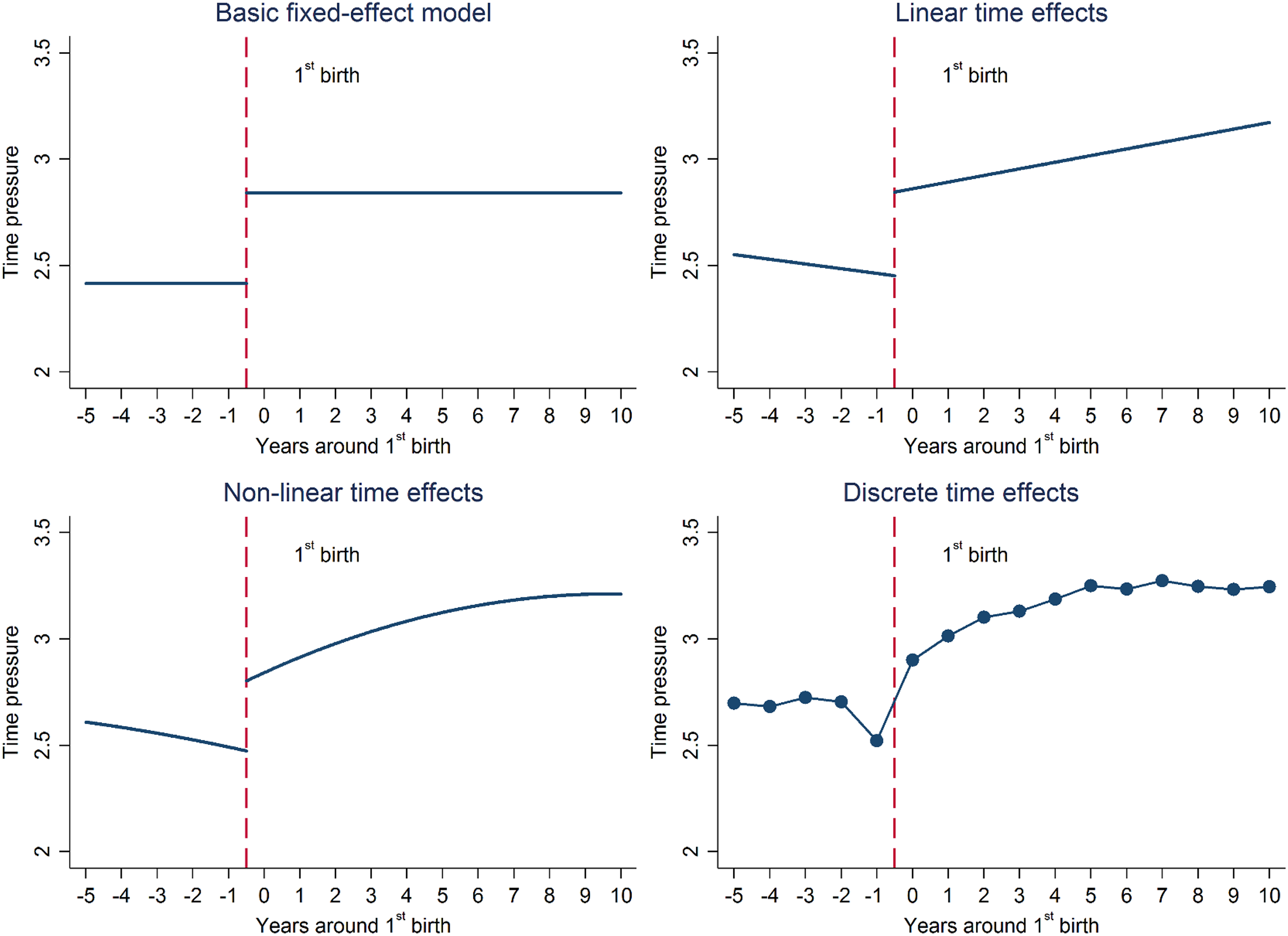
Comparison of model specifications. Note. Household, Income and Labour Dynamics in Australia Survey, 2001–2016. Model predictions with covariate values held at their means.

The predictions of the base fixed effects model (top-left panel) show a clear average difference in time pressure before and after parenthood. As seen in column 3, this difference is statistically significant (Model 3: β = .427; p < .001). Yet this depiction of the process seems rather crude when compared to that provided by the model introducing linear time effects (top-right panel). This offers two new and perhaps important pieces of information there is: (i) a statistically significant decline in time pressure preceding the transition to parenthood (Model 4: β = −.022; p < .001), and (ii) a statistically significant upward increase in time pressure with time since parenthood (Model 4: β = .031; p < .001). This model also provides an estimate of the immediate change associated with parenthood, which in this case is substantial and statistically significant (Model 4: β = .420; p < .001). This upward “shock” in women’s time pressure between the year immediately before and the year immediately after parenthood is more pronounced than in the basic fixed effects model.

The graph in the bottom-left panel shows results from the model that allows the trends before and after parenthood to follow a quadratic function (Model 5). These suggest some nonlinearities post-parenthood, whereby time pressure increases rapidly up to around 5 years after the birth, and then remains stable. This nonlinear effect is statistically significant, as can be appreciated by inspecting the p-value on the coefficient on the quadratic term in column 5 (Model 5: β = −.004; p < .001). There is nevertheless no evidence of nonlinear relationships pre-parenthood—as evidenced by a statistically insignificant coefficient on the relevant quadratic term (Model 5: β = .002; p > .05).

Finally, the results in the bottom-right panel are for the nonparametric model specification using time dummies (Model 6), which does not impose a functional form on the pre- and post-parenthood trajectories. In this occasion, its results are very similar to those of the previous model—though they further stress the reduction in time pressure experienced by mothers-to-be in the year preceding the birth.

Understanding couple-level processes: The promise of longitudinal dyadic models

The transition to parenthood is often experienced in parallel by two individuals within a couple relationship. As such, many key research questions in this space pertain to couple-level processes. For example, researchers may seek to understand how partner characteristics affect individuals’ post-parenthood adjustment, or whether the pace of any longitudinal adjustment differs between the partners within each couple. Answering these questions requires conceptualizing the transition to parenthood as a “dyadic” process (Kenny, Kashy, & Cook, 2006).

Naturally, dyadic modeling requires data from two members of a dyad, and such data are less often available than the individual-level data required to fit the panel regression models discussed thus far. Fortunately, many existing panel data sets not only track individuals over time, but also their partners. For example, household panel studies such as the U.S. Panel Study of Income Dynamics, the German Socio-Economic Panel, the BHPS, and the HILDA Survey interview complete households. These data, as well as other purposively collected primary data, enable researchers to model the transition to parenthood as a longitudinal and a dyadic process at the same time. Although dyadic models are most often deployed in cross-sectional applications, extensions for longitudinal data are rapidly emerging (Kammrath, Curran, & Laurenceau, 2018; West, 2013). These approaches can be—but have seldom been—used to model the transition to parenthood.

Use of longitudinal dyadic models in this context has significant methodological advantages. First, it relaxes the regression assumption of independence across observations (Kenny et al., 2006, pp. 4–5). Information from couple members is clearly dependent: Their child is the same and they may share a common residence, plus they may be more alike to each other than to other individuals in the data (e.g., through assortative mating). Second, it can accommodate more complex theoretical models in which the consequences of parenthood on an individual are not only determined by her/his own traits and behaviors, but also by those of the other parent (Kenny et al., 2006, p. 2).

Most applications of longitudinal dyadic modeling to the transition to parenthood fall within the standard one-to-one actor-partner design, with parenthood and its associated variables (e.g., time to/since parenthood) being between-dyad variables that differ across but not within dyads. The outcomes of interest could be reciprocal (e.g., satisfaction with partner) or nonreciprocal (e.g., time pressure). The key methods to model data with this structure and properties can be seen as extensions of multilevel models (Ledermann & Kenny, 2017), of which the panel regression models discussed thus far are a special case. Yet longitudinal dyadic models are computationally demanding and their estimation often requires specialized software—such as Amos, MLwiN, or Mplus.

A longitudinal extension of the most widespread dyadic model, the overtime actor–partner interdependence model (APIM), is described in detail in the work of Cook and Kenny (2005). This model—sometimes referred to as the stability and influence model (West, 2013)—separates the effects of the characteristics of a person (the actor) and a partner on the person’s and the partner’s outcomes at different time points. It also quantifies correlations between the random intercepts for each partner. However, because the focus here is on between-dyad variables capturing parenthood that have common scores for both partners, the advantages of this approach to understanding parenthood main effects are modest. Further, these models tend to be restricted to two observation points (Cook & Kenny, 2005). Modeling interaction effects between covariates of interest and variables measuring parenthood (or time before/since parenthood) is nevertheless useful to compare the bidirectional influences of a person’s and a partner’s characteristics on each other’s outcomes before and after parenthood (see Cook & Kenny, 2005).

A second dyadic specification, one that brings more explicit longitudinal insights of potential interest in transition-to-parenthood research, is the dyadic growth model (for details, see Kenny et al., 2006, Ch. 13; Lyons & Sayer, 2005). In our context, this model can be leveraged to measure change over time (or “growth”) in a given outcome for the two parents as a function of time before/around/after parenthood and to identify correlations between the parents’ growth/change trajectories. Different versions of growth models are possible with longitudinal, dyadic data—including correlated growth models (which estimate separate but correlated growth trajectories for each partner) and common-fate growth models (which treat the dyad as the unit of analysis) (Gray & Ozer, 2018; see also Galovan, Holmes, & Proulx, 2017; West, 2013).

Empirical applications of dyadic longitudinal models in research examining the consequences of the transition to parenthood are, however, scarce. One exception is the work of Keizer and Schenk (2012), who applied longitudinal dyadic growth models to BHPS data to compare how men’s and women’s relationship satisfaction was affected by parenthood, and how changes in paid and domestic work hours affected personal and partner’s outcomes across the transition to parenthood. Another exemplar is Le, McDaniel, Leavitt, and Feinberg (2016), which examined relationship quality and co-parenting across the transition to parenthood applying an overtime APIM to a sample of 164 couples observed at pregnancy, 6 months after parenthood, and 3 years after parenthood.

Longitudinal dyadic methods can also be adapted to accommodate more complex data structures, such as indistinguishable dyads for which there is no clear ordering (Kenny et al., 2006, pp. 6–7). In transition-to-parenthood research, this is important for analyses of same-sex couples—where gender cannot be used as an ordering variable. An example application can be found in the study by Goldberg and Smith (2011), where an adapted dyadic growth model for indistinguishable dyads was deployed on a sample of 90 same-sex couples to examine parental mental health at three time points within the first year of adoptive parenthood.

Although still incipient and methodologically complex, longitudinal dyadic modeling may prove extremely useful to test important theoretical tenets concerning the transition to parenthood. For instance, this approach aligns with the core principle of “linked lives” from life-course theory, which poses that individuals and their significant others occupy mutually influential and interlocking life trajectories (Elder et al., 2003). Longitudinal dyadic models are thus enviably placed to ascertain whether and how the consequences of parenthood for an individual are influenced by the behaviors, traits, and outcomes of their partner, and whether any associations change over time. Longitudinal dyadic models can also inform transition-to-parenthood research inspired by family systems theory (Minuchin, 1988). For example, they can be used to address questions such as “how does the husband-wife subsystem adapt to disruptions stemming from parenthood”? or “at which points in time is adaptive self-organization most likely to manifest?” (Cox & Paley, 1997, pp. 250–252). These models are also fit-for-purpose to test hypotheses concerned with interindividual stress contagion, as depicted in the stress process model (Bolger, DeLongis, Kessler, & Wethington, 1989)—for instance, whether and how the stress and time pressure associated with parenthood spillover from one spouse to another.

Conclusion

In this article, I have introduced and discussed a selection of panel regression methods available to family researchers interested in understanding the social and economic consequences of the transition to parenthood when panel data are available. Table 2 in Online Appendix 3 summarizes the properties, advantages, and disadvantages of all of the approaches discussed. With panel data, researchers can move from undertaking comparisons of parents and nonparents to examining the transition to parenthood as a longitudinal process with ramifications that stretch over time—both in the short- and long-run. A basic use of the panel data is to utilize the repeated measurements on the same individuals to fit panel regression models that improve estimation of the parenthood effects—such as random or fixed effects models. More importantly, having a window into the lives of the same individuals and their partners over prolonged periods of time can be used to develop and test more complex causal hypotheses about how the consequences of parenthood unfold and spillover. The modeling approaches discussed later in the article, including longitudinal piecewise and dyadic models, are ripe for researchers to incorporate new theoretical ideas into empirical analyses, thereby enhancing their ability to tackle novel questions that involve temporal complexities in how parenthood relates to personal, couple, or family outcomes.

Supplemental material

Online_appendix_supplementary_material - Modeling the consequences of the transition to parenthood: Applications of panel regression methods

Online_appendix_supplementary_material for Modeling the consequences of the transition to parenthood: Applications of panel regression methods by Francisco Perales in Journal of Social and Personal Relationships

Footnotes

Acknowledgements

The author would like to thank Alice Campbell, Wojtek Tomaszewski, Martin O’Flaherty, Stefanie Plage and Janeen Baxter for helpful comments and suggestions. This research was supported by the Australian Research Council Centre of Excellence for Children and Families over the Life Course (project number CE140100027). The paper uses data from the Household, Income and Labour Dynamics in Australia (HILDA) Survey. The HILDA Project was initiated and is funded by the Australian Government Department of Social Services (DSS) and is managed by the Melbourne Institute of Applied Economic and Social Research (Melbourne Institute). The findings and views reported in this paper, however, are those of the author and should not be attributed to either DSS or the Melbourne Institute.

Funding

The author received no financial support for the research, authorship, and/or publication of this article.

ORCID iD

Francisco Perales

Open research statement

As part of IARR’s encouragement of open research practices, the author has provided the following information: This research was not pre-registered. The data used in the research are available and can be obtained from the Melbourne Institute of Applied Economic and Social Research at The University of Melbourne after obtaining a license; see . The materials used in the research are available and can be obtained by emailing the author at f.perales@uq.edu.au.

Supplemental material

Supplemental material for this article is available online.

References

Allison

P. D.

(2009). Fixed effects regression models (Vol. 160). Los Angeles, CA: Sage.

Allison

P. D.

(2014). Event history and survival analysis: Regression for longitudinal event data (Vol. 46). Los Angeles, CA: Sage.

Baxter

Buchler

Perales

Western

. (2015). A life changing event: First births and men’s and women’s attitudes to mothering and gender divisions of labor. Social Forces, 93, 989–1014. doi:10.1093/sf/sou103

Baxter

Hewitt

Haynes

. (2008). Life course transitions and housework: Marriage, parenthood, and time on housework. Journal of Marriage and Family, 70, 259–272. doi:10.1111/j.1741-3737.2008.00479.x

Bell

Jones

(2015). Explaining fixed effects: Random effects modeling of time-series cross-sectional and panel data. Political Science Research and Methods, 3, 133–153. doi:10.1017/psrm.2014.7

Bolger

DeLongis

Kessler

R. C.

Wethington

(1989). The contagion of stress across multiple roles. Journal of Marriage and the Family, 51, 175–183. doi:10.2307/352378

Bollen

K. A.

Curran

P. J.

(2006). Latent curve models: A structural equation perspective. Hoboken, NJ: Wiley.

Breusch

T. S.

Pagan

A. R

. (1979). A simple test for heteroskedasticity and random coefficient variation. Econometrica, 47, 1287–1294. doi:10.2307/1911963

Claxton

Perry-Jenkins

. (2008). No fun anymore: Leisure and marital quality across the transition to parenthood. Journal of Marriage and Family, 70, 28–43. doi:10.1111/j.1741-3737.2007.00459.x

10.

Cook

W. L.

Kenny

D. A.

(2005). The actor–partner interdependence model: A model of bidirectional effects in developmental studies. International Journal of Behavioral Development, 29, 101–109. doi:10.1080/01650250444000405

11.

Cox

M. J.

Paley

. (1997). Families as systems. Annual Review of Psychology, 48, 243–267. doi:10.1146/annurev.psych.48.1.243

12.

Delicate

Ayers

McMullen

. (2018). A systematic review and meta-synthesis of the impact of becoming parents on the couple relationship. Midwifery, 61, 88–96. doi:10.1016/j.midw.2018.02.022

13.

Elder

G. H.

Johnson

M. K.

Crosnoe

(2003). The emergence and development of life course theory. In Mortimer

Shanahan

(Eds.), Handbook of the life course (pp. 3–19). Boston, MA: Springer.

14.

Galovan

A. M.

Holmes

E. K.

Proulx

C. M

. (2017). Theoretical and methodological issues in relationship research: Considering the common fate model. Journal of Social and Personal Relationships, 34, 44–68. doi:10.1177/0265407515621179

15.

Goldberg

A. E.

Smith

J. Z.

(2011). Stigma, social context, and mental health: Lesbian and gay couples across the transition to adoptive parenthood. Journal of Counseling Psychology, 58, 139. doi:10.1037/a0021684.

16.

Goldstein

(2011). Multilevel statistical models (Vol. 922). Hoboken, NJ: John Wiley & Sons.

17.

Gould

StataCorp. (n.d.). Interpreting the intercept in the fixed-effects model. Retrieved from https://www.stata.com/support/faqs/statistics/intercept-in-fixed-effects-model/

18.

Gray

J. S.

Ozer

D. J.

(2018). Comparing two models of dyadic change: Correlated growth versus common fate. Forthcoming in Social Psychological and Personality Science . doi:10.1177/1948550618799066

19.

Hausman

J. A

. (1978). Specification tests in econometrics. Econometrica, 46, 1251–1271. doi:10.2307/1913827

20.

Hewitt

Baxter

Western

. (2006). Family, work and health: The impact of marriage, parenthood and employment on self-reported health of Australian men and women. Journal of Sociology, 42, 61–78. doi:10.1177/1440783306061353

21.

Hynes

Clarkberg

. (2005). Women’s employment patterns during early parenthood: A group-based trajectory analysis. Journal of Marriage and Family, 67, 222–239. doi:10.1111/j.0022-2445.2005.00017.x

22.

Jung

Wickrama

K. A. S.

(2008). An introduction to latent class growth analysis and growth mixture modeling. Social and Personality Psychology Compass, 2, 302–317.

23.

Kammrath

L. K.

Curran

M. A.

Laurenceau

J. P

. (2018). Introduction to the special issue: Data analytic issues in relationship research. Journal of Social and Personal Relationships, 35, 3–6. doi:10.1177/0265407517734399

24.

Keizer

Schenk

. (2012). Becoming a parent and relationship satisfaction: A longitudinal dyadic perspective. Journal of Marriage and Family, 74, 759–773. doi:10.1111/j.1741-3737.2012.00991.x

25.

Kenny

D. A.

Kashy

D. A.

Cook

W. L.

(2006). Dyadic data analysis. New York, NY: Guilford.

26.

Lawrence

Nylen

Cobb

R. J.

(2007). Prenatal expectations and marital satisfaction over the transition to parenthood. Journal of Family Psychology, 21, 155–164. doi:10.1037/0893-3200.21.2.155

27.

McDaniel

B. T.

Leavitt

C. E.

Feinberg

M. E

. (2016). Longitudinal associations between relationship quality and coparenting across the transition to parenthood: A dyadic perspective. Journal of Family Psychology, 30, 918–926. doi:10.1037/fam0000217

28.

Ledermann

Kenny

D. A

. (2017). Analyzing dyadic data with multilevel modeling versus structural equation modeling: A tale of two methods. Journal of Family Psychology, 31, 442. doi:10.1037/fam0000290

29.

Lyons

K. S.

Sayer

A. G

. (2005). Longitudinal dyad models in family research. Journal of Marriage and Family, 67, 1048–1060. doi:10.1111/j.1741-3737.2005.00193.x

30.

Minuchin

(1988). Relationships within the family: A systems perspective on development. In Hinde

R. A.

Stevenson-Hinde

(Eds.), Relationships within families: Mutual influences (pp. 7–26). Oxford, UK: Oxford University Press.

31.

Nomaguchi

Milkie

M. A

. (2003). Costs and rewards of children: The effects of becoming a parent on adults’ lives. Journal of Marriage and Family, 65, 356–374. doi:10.1111/j.1741-3737.2003.00356.x

32.

Nowok

Van Ham

Findlay

A. M.

Gayle

. (2013). Does migration make you happy? A longitudinal study of internal migration and subjective well-being. Environment and Planning A, 45, 986–1002. doi:10.1068/a45287

33.

Pearlin

L. I.

(2009). The life course and the stress process: Some conceptual comparisons. Journals of Gerontology Series B: Psychological Sciences and Social Sciences, 65, 207–215. doi:10.1093/geronb/gbp106

34.

Perales

del Pozo-Cruz

. (2015). Long-term dynamics in physical activity behavior across the transition to parenthood. International Journal of Public Health, 60, 301–308. doi:10.1007/s00038-015-0653-3

35.

Plage

Perales

Baxter

(2016). Doing gender overnight? Parenthood, gender and sleep quantity and quality in Australia. Family Matters, 97, 73–81.

36.

Rabe-Hesketh

Skrondal

(2008). Multilevel and longitudinal modeling using Stata. College Station, TX: Stata Press.

37.

Raudenbush

S. W.

Bryk

A. S.

(2002). Hierarchical linear models: Applications and data analysis methods (2nd ed.). London, UK: Sage.

38.

Rossi

A. S

. (1968). Transition to parenthood. Journal of Marriage and the Family, 30, 26–39. doi:10.2307/350219.

39.

Ruppanner

Perales

Baxter

(2019). Harried and unhealthy? Parenthood, time pressure and mental health. Journal of Marriage and Family, 81, 308–326. doi:10.1111/jomf.12531.

40.

Schunck

Perales

(2017). Within-and between-cluster effects in generalized linear mixed models: A discussion of approaches and the xthybrid command. Stata Journal, 17, 89–115.

41.

Snijders

T. A. B.

Bosker

R. J.

(1999). Multilevel analysis. An introduction to basic and advanced multilevel modelling. Thousand Oaks, CA: Sage.

42.

Tan

Shiyko

M. P.

Dierker

. (2012). A time-varying effect model for intensive longitudinal data. Psychological Methods, 17, 61–77. doi:10.1037/a0025814

43.

Vidal

Perales

Baxter

. (2016). Dynamics of domestic labour across short- and long-distance family relocations. Journal of Marriage and Family, 78, 364–382. doi:10.1111/jomf.12269

44.

West

T. V.

(2013). Repeated-measure methods with dyads. In Simpson

J. A.

Campbell

(Eds.), The Oxford handbook of close relationships (pp. 731–749). New York, NY: Oxford University Press.

45.

Wooldridge

J. M.

(2010). Econometric analysis of cross section and panel data. Cambridge, MA: MIT Press.

Supplementary Material

Please find the following supplemental material available below.

For Open Access articles published under a Creative Commons License, all supplemental material carries the same license as the article it is associated with.

For non-Open Access articles published, all supplemental material carries a non-exclusive license, and permission requests for re-use of supplemental material or any part of supplemental material shall be sent directly to the copyright owner as specified in the copyright notice associated with the article.

0.00 MB

0.49 MB