
Abstract
This paper discusses a project on the completion of a database of socio-economic indicators across the European Union for the years from 1990 onward at various spatial scales. Thus the database consists of various time series with a spatial component. As a substantial amount of the data was missing a method of imputation was required to complete the database. A Markov Chain Monte Carlo approach was opted for. We describe the Markov Chain Monte Carlo method in detail. Furthermore, we explain how we achieved spatial coherence between different time series and their observed and estimated data points.
Introduction
Article 174 of the Lisbon Treaty states “In order to promote its overall harmonious development, the Union shall develop and pursue its actions leading to the strengthening of its economic, social and territorial cohesion” (EU, 2008). To achieve this will entail the reduction of disparities between levels of development of its regions; these regions include rural areas, areas affected by industrial transition, and regions with natural or demographic handicaps. The creation of suitable policies towards this goal, the evaluation of alternative policies, their implementation and monitoring require a solid base of evidence.
Article 2 of the European Territorial Cooperation Regulation 1299/2013 calls for interregional cooperation to reinforce the effectiveness of cohesion policy by promoting “analyses of development trends in relation to the aims of territorial cohesion, including territorial aspects of economic and social cohesion, and harmonious development of the European territory through studies, data collection and other measures” (EU, 2013).
Among the activities, and which shall be the focus of this paper, has been the creation of a database under the ESPON (European Spatial Planning Observation Network) 2013 programme (ESPON, 2016) of socio-economic indicators across the 28 member states of the European Union for each year from 1990 onwards. Those indicators include figures on population, birth and death rates, migration, GDP as well as employment and unemployment rates. The database can then be used as a tool to support policy design in relation to the aim of territorial cohesion and a harmonious development of the European territory. It provides comparable information, evidence, analyses and scenarios on regional dynamics and reveals territorial capital and potentials for the development of smaller and larger regions contributing to European competitiveness, territorial cooperation and a sustainable and balanced development.
Each of the 28 countries under consideration is subdivided into NUTS regions (NUTS, for the French nomenclature d’unites territoriales statistique, that is, Nomenclature of Territorial Units of Statistics) of up to three levels with increasing degrees of division. These different levels are called NUTS1, NUTS2 and NUTS3, that is, first-level, second-level and third-level regions, respectively, with NUTS0 usually denoting the entire country. For instance, Ireland is divided into two NUTS1 regions, which in turn are divided into three and five NUTS2 regions, respectively. Due to its relatively small size, there are no NUTS3 regions in Ireland. In comparison, Germany has 16 NUTS1, 39 NUTS2 and 429 NUTS3 regions.
The objective of the project was to produce a space-time series on an annual basis for each NUTS region and for each of the indicators starting in the year 1990. A large amount of the required datasets is readily available for a variety of spatial scales and can be obtained from EUROSTAT or the relevant National Statistical Offices. It is desirable that they are not only complete in their temporal domain, but also internally coherent in the spatial domain. However inspection of the series revealed that some data were missing for parts of the time periods and spatial scales of interest. There might be several reasons for this lack of completeness such as population censuses only being carried out every five years in some countries like Ireland or even every 10 years as is the case in the UK. Also while national and regional population estimates may be provided by national agencies, data at lower levels (NUTS2 and NUTS3) are less common.
Clearly this incompleteness of the data provides a challenge for an analyst who tries to extract useful information from the data. In survey analysis, a common strategy is to analyse only those cases with complete data for the variables of interest. This raises the question as to whether the mechanism for creating the missing variables is a random process. If it is not, then the possibility of introducing bias into the analysis becomes a problem. Furthermore, as in our case most of the data are missing at NUTS3 level, analysis on a more local level becomes increasingly difficult.
Hence it was the task of this research team to develop an internally coherent methodology which achieves the twin goals of imputing the missing data and ensuring the internal spatial coherence of the data. We opted for a Bayesian approach using a Markov Chain Monte Carlo (MCMC) algorithm. Furthermore, we implemented the algorithm using JAGS (Just Another Gibbs Sampler) software which can be interfaced to R. Finally, due to the nature of the ESPON data, more work needed to be done in order to ensure that the observed and imputed data satisfy spatial coherence, that means, in each year the sum of the observed and/or predicted values of all regions at one NUTS level that are constituents (children) of the same region X at the next higher NUTS level (parent) must equal the corresponding value of that region X. In particular, an algorithm had to be developed to guarantee spatial coherence within the data.
We start this paper by giving a brief general introduction to time series. Next we focus on the character of the ESPON data and some of the issues that arose from its particular nature. Clearly there are many possible imputation methods that could be applied to predict missing data in a given time series with unobserved data. We discuss some of the available methods and why we did not choose to use them. Finally, we present the model and the algorithm which we applied to impute missing data in our time series. Also we show how we dealt with the issue of spatial coherence before we conclude the paper by presenting our results.
Time series
A time series is a collection of observations or data points made sequentially in time (Chatfield, 1989). Time series are frequently encountered in (i) economics (Beveridge annual wheat price series), (ii) physical sciences (monthly average air temperature), (iii) marketing (monthly product sales), (iv) demography (annual population estimates), (v) process control (weights of manufactured product sampled hourly) and (vi) communication (binary series are common). While many series are usually measured at regular intervals (e.g.: year, month, week, day, hour, minute), there are series which occur irregularly, for example, major railway disasters, which are known as point processes.
Time series analysis is concerned with (i) description of the main properties of the series, (ii) explanation of the relationship between two series taken at the same time (monthly atmospheric temperature readings, monthly measurements of the North Atlantic Oscillation) and (iii) prediction of (usually) future values.
Time series description can take several forms, but are intended to reveal the underlying structure of the series. This structure can include several components (Shumway and Stoffer, 2010); (i) Trend, that is, an increase or decrease in the value of the series over time, (ii) Seasonality, that is, a regular pattern of high and low values related to calendar time, (iii) Long term cycles, that is, periodicity not related to seasonality, (iv) Outliers, that is, values which are unusually high or low in comparison with the rest of the data, (v) Abrupt changes, that is, changes to the variation in the series or level and (vi) Variance, that is, the extent of the spread of the data.
Often it may happen that some time series in a data set are incomplete. Naturally, this complicates any further analysis of the data. In Enders (2010), it is noted that the analyst should make the distinction between the missing data pattern and the missing data mechanism. He proceeds to explain that the pattern relates to the configuration of observed and unobserved data, whereas the mechanism permits a description of the relationship between the two in terms of probability. Rubin (1976) proposed to classify missing data mechanisms into three types: (1) missing at random (MAR), (2) missing completely at random (MCAR) and (3) missing not at random (MNAR). Somewhat misleadingly MAR does not describe that data is missing in a haphazard way, but instead arises when the probability of missing data on some variable X is related to the values of some other measured variable Y in the dataset but not on the values of X itself. As an example, we could think of a survey in which variable Y asks for one’s age and one only has to answer question X if one is past a certain age. The MCAR mechanism arises when the probability of missing data on some variable X is unrelated to any other variable in the dataset, including the variable X itself. In fact, this mechanism describes “purely haphazard missingness” (Enders, 2010). Finally, MNAR arises when the probability of missing data on a variable X is related to the values of the variable itself. Enders uses an example of cancer patients in a trial becoming so ill that they are unable to continue participation in the trial. The ESPON time series missing data are likely to arise from an MCAR process, as missingness in the data, though often temporally correlated, is statistically independent of other data in the dataset. So are for instance population values at NUTS3 level not missing because they were too small or too big to be collected (which would be a case of MNAR), nor because data collected in previous years were too small or too big (which would be a case of MAR), but instead a lack of resources or a lack of political will to collect the data at the smallest level may have been the driving force for the omission.
The character of the ESPON data
As described in the introduction, the purpose of this ESPON project was to build up a database with annual figures on socio-economic indicators such as population, birth and death rates, employment and unemployment rates and GDP for all 28 EU member states for each year from 1990 onwards. Hence we have a maximum of 25 observations per time series, which must be considered as short. Furthermore each country is divided and further sub-divided into at most three NUTS levels. Across the entire EU, we have 28 NUTS0 regions (countries), 98 NUTS1 regions (major socio-economic regions), 273 NUTS2 regions (area for application of region policy) and 1324 NUTS3 regions (smaller regions).
Through a hierarchical coding system, it is clear which NUTS1 region contains which NUTS2 regions and which NUTS2 region contains which NUTS3 regions. In fact, every country has its own letter code, for instance, The Netherlands have NL. There are four NUTS1 regions in The Netherlands which are called NL1, NL2, NL3 and NL4, respectively. Next the NUTS1 region NL3, for instance, contains four NUTS2 regions, which are labelled NL31, NL32, NL33 and NL34, respectively. Those NUTS2 regions in turn contain different numbers of NUTS3 regions. For instance, NL31 contains no NUTS3 region, while NL32 contains the seven NUTS3 regions NL321 to NL327.
For the purpose of running algorithms on the dataset, it is helpful to represent the NUTS structure in a tree. Trees are used widely in computer science for organising and searching for information. In “The Art of Computer Programming”, Knuth (1973) defines a tree as a finite set T of one or more nodes such that
there is one specially designated node called the root of the tree; and the remaining nodes (excluding the root) are partitioned into m disjoint sets
This definition is recursive as a tree is defined in terms of trees. Put another way: a tree consists of a root and one or more nodes, each of which is a tree. A root which has no nodes is called a leaf node. There is an analogy with a family tree, a structure much used in genealogy: the non-root nodes are the children and the root represents the parents. As each node is itself a tree, we can also refer to the nodes as subtrees.
The NUTS hierarchy can be represented as a tree quite naturally in terms of this definition. A node consists of the NUTS code, the NUTS level and a socio-economic indicator such as the national population. The root would be the EU and its 28 nodes are comprised by the 28 NUTS0 regions. Each of these 28 nodes is itself a tree. Each NUTS0 node has one or more NUTS1 nodes, and in turn each NUTS1 node has one or more NUTS2 nodes and so on. See Figure 1 for a hypothetical example.
The NUTS tree for a hypothetical country labelled X.
As far as possible, the data for the various indicators and NUTS regions were collected from the EUROSTAT website or national statistical agencies. Data from EUROSTAT were always given preference, however, sometimes national agencies would provide data for more years than were available through EUROSTAT. For instance, in the case of the Finish NUTS3 region FI193 population values are available from EUROSTAT for the years 2000–2012, but the national statistical agency provides values from 1991 onwards. In such a case, we compare national values and EUROSTAT values where they overlap and if they agree then national values may be used with confidence.
Throughout this paper, we discuss our method and observation with respect to the population indicator. Figure 2 shows how much data in the case of the population figures are missing at each NUTS level. For instance, we see that all NUTS0 series are complete, however gaps in the series become increasingly frequent as we move down the hierarchy. Especially at the NUTS3 level, the situation has deteriorated to a degree that some series miss at least half of their data.
Number of instances of missing data for each NUTS level in the entire population database.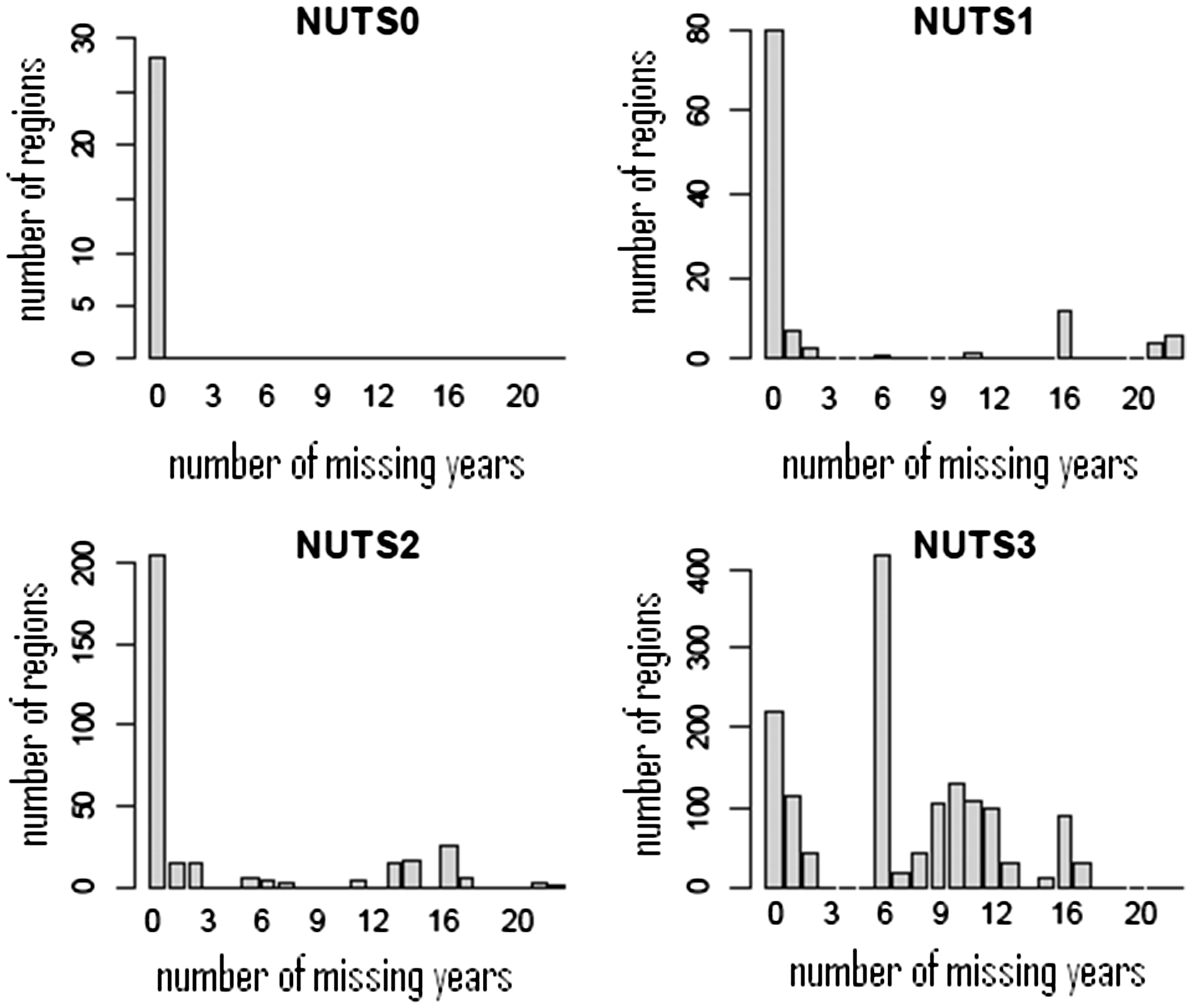
Also the pattern of missing data causes problems as data might be missing at the beginning of a time series, in the middle, at the end or some combination of these. For instance, many East-European countries miss a substantial portion of their data in the early part of the time period. This variety in the pattern of missing data requires a method that allows us to predict all types of missing data in one consistent way.
Another key issue is that the ESPON data are characterised by both a temporal and a spatial component. The temporal component is the trend of the data as years pass. This trend may be upwards, downwards or either at different times throughout the period of 25 years and for each NUTS region the corresponding time series will hold that information. On the other hand, we have a spatial component. This is due to the fact that usually a NUTS region of a particular level (parent) consists of several NUTS regions of the next lower level (children). Hence in each year the value of a parent must equal the sum of the respective values of all its children, that is, all those regions that constitute the parent. This spatial hierarchy of parent and child NUTS regions introduces an additional constraint on any prediction we make. In particular, this spatial coherence is a vital part of a consistent database.
In some instances, this spatial component allows us to solve some of the gaps in a series directly by using the data of either the children to determine the missing values of the parent or using the data of the parent and some children to determine the value of another child. For instance, on some occasion a NUTS2 entry might be unobserved in the data but the value for all NUTS3 regions that constitute the NUTS2 region are known. In this case, the value of the NUTS2 region is the sum of the values for all the relevant NUTS3 regions. This for instance occurred with the Croatian population figures in the year 2001, where the values for all NUTS2 and NUTS3 regions are available in the comprised database but the values for the three NUTS1 regions are missing. Clearly the value for each NUTS1 region can then be recovered but adding up the values of all its children at the NUTS2 level. Similarly if the value for a NUTS1 region and one of its two NUTS2 regions is known, the missing value for the second NUTS2 region can be derived by subtracting the observed value of the first NUTS2 region from the observed value of the NUTS1 region.
Once the whole observed data has been transferred into a coherent initial database, an program was written to search for and fix such self-solving problems. Here the tree structure of the NUTS hierarchy can be exploited. At each NUTS level, starting with NUTS0, we visit each parent. The coding system defines a natural order on the regions of a particular NUTS level which we can exploit. If for instance, the NUTS2 regions are X11, X12, X13, X21 and X22, then we visit them in this very order. Now for each parent and all its children, we check how many values are unobserved. If all but one values are present, the missing value can be calculated from the observed values. Note that if the calculated value is that of a child, the algorithm continues with the next parent in line. If however the calculated value is that of the parent, then we need to move back up the hierarchy to the parent’s parent, if possible, and continue the algorithm from there. This is necessary as the newly calculated parent is the child in a previously checked part of the tree which now requires rechecking. The algorithm ends once we have dealt with the last parent on the NUTS2 level.
Ultimately we are left with a large number of time series which (a) are incomplete in parts and where the missing data cannot be derived logically from the observed data and (b) are restricted by the issue of spatial coherence, which is imposed by the tree structure of the NUTS hierarchy.
Possible methods of dealing with missing data
Traditional methods for dealing with missing data include deletion methods and imputation methods. Both types are described in more detail in Enders (2010). The two most common deletion methods are listwise and pairwise deletion (Peugh and Enders, 2004). Listwise deletion, or complete case analysis, removes any observation with one or more missing values. A variant of this approach is pairwise deletion, or available-case analysis, which removes variables on an analysis-by-analysis case. The problem with either method is that it often introduces bias into the data set if the process that causes the data is not random. Furthermore in the case of pairwise deletion it results in the correlations in a correlation matrix potentially being based on different numbers of underlying observations (Little 1992; Marsh, 1998).
Another issue with deletion methods is that they wastefully reduce the sample size and thus mitigates the power of statistical methods. Especially in a case as ours, where the ESPON dataset is relatively small, an analyst cannot afford to further lose data. Hence an attempt at completing the missing data by the use of some imputation methods may be more sensible. Such methods include Mean/Median substitution, regression imputation, (and stochastic regression imputation which adds a random number from the distribution of residuals), hot-deck imputation (scores are taken from similar complete observations) or the method of last observation carried forward (LOCF).
Arithmetic mean imputation suggests the replacement of missing data by the arithmetic mean of the series. This however has widely been found to introduce bias into the data set (Brown, 1994; Enders and Bandalos, 2001; Gleason and Staelin, 1975). For instance, in our case, it is clear that this method fails to deliver a good estimate for missing data at the beginning of the series if the series has an overall rising trend. Also the missing data might be in the middle of the series and due to a change in trend throughout the series the mean could differ substantially from the closest observed data point on either side of the missing data. Replacement by the mean or the median of only nearby observations raises the questions of how many observed data points to use in the calculation and what if there are not enough. Also should observations that are closer to a missing point be considered more relevant? This is further complicated if data is missing in the middle of the series and there are nearby observations on either side. If for instance the years 2000–2005 are missing in an otherwise complete time series and we wish to impute the value for the year 2000, should the observed value of 2006 be used and if yes with what weighting? Again, if data is missing at the beginning of the series with a rising trend in the observed data, then replacing the missing data by the mean of any number of nearby observations would create a picture, which completely ignores the trend. Linear interpolation could be helpful in certain cases but will for instance struggle with missing data in the middle of the series if trends change from downwards to upwards or vice versa.
With the method of hot-deck imputation (Ford, 1983; Little and Rubin, 2002), the nearest matching record, with complete data, to the record with missing data is identified, and the missing data copied from the complete to the incomplete record. In our case, this method is difficult to implement as most time series miss data during the 1990s. Furthermore this approach completely disregards the fact that the time series hold data of a vast variety of different regions across a very diverse Europe. In particular, there is no reason to assume that a trend that occurred in some region in Ireland during the 1990s should therefore also have occurred in some region of Bulgaria. Generally, as noted in (Enders, 2010), hot-deck methods have been found to produce substantially biased estimates of correlation and regression coefficients (Brown, 1994; Schafer and Graham, 2002).
In the case of LOCF, the data value in the last non-missing time period is copied into the missing parts of the series. Like hot-deck imputation, this is an expedient method and it fails to encapsulate the underlying missing data generating processes satisfactorily (Cook et al., 2004; Liu and Gould, 2002; Molenberghs et al., 2004). In a variation of LOCF, one may exploit the NUTS spatial hierarchy. For instance if data is missing at a NUTS3 level, but there is data for the containing NUTS2 region, then one might propagate the proportional split of the NUTS3 values backwards from the last time period with complete data. If there are missing observations in the middle of the series, the proportionate split can be estimated by pro-rata from the known data beyond the immediate endpoints of missing time periods. Again, these are expedient approaches and do not allow us to make full use of the evidence provided by all the data in each series. Also despite some of these approaches possibly working well in some instances of missing data we are likely to encounter in the ESPON project, they fail to deal with all cases in one consistent way.
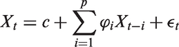
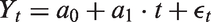
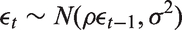
Therefore a model based approach is desirable and one might consider a regression imputation. In an autoregressive model, the value of the series at time t depends on p previous values:
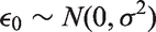
By contrast in a moving average model, the error at time t depends on q previous values:
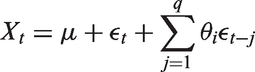
These can be combined to give an autoregressive moving average model:

Such models were given extensive treatment in Box and Jenkins (1970). They are conventionally fitted to a series which is stationary (that is, in which the trend has been removed), a situation obtained by differencing. If the trend is linear, the series might need to be differenced once (i.e.
Due to the shortness of at most 25 data points in an ESPON series we do not have this luxury. In fact many time series that require estimating have less than 15 data points with observed values. Hence there is insufficient data to provide reliable estimates for the parameters of an autoregressive or moving average model. Also the varying pattern of the missing data points in the series complicates things further, suggesting that these traditional approaches of analysis are not suitable. For example, in a particular NUTS3 region, data might be missing for intercensal years in the 1990s: 1990, and 1992 to 2000 inclusive, so that the evidence we have is the single value in 1991 and the series from 2001 to 2012. However, data may be present for the containing NUTS2 region for the entire time period. The problem becomes one of identifying a technique which will allow us to make use of all the available evidence in a coherent and consistent fashion.
If we can model the trend in the existing data and any autocorrelations in the residuals after the trend is removed, then we have the basis for both estimating missing data and providing an estimate for the uncertainty. As we have noted above, the series are too short for traditional time series methods. Furthermore we do not know the statistical properties of the series, except that they are unlikely to arise from an independent and identical distributed process. For these reasons, we choose a forecasting strategy based on Bayesian methods.
A Bayesian approach
Markov Chain Monte Carlo
Assume we have given a data set D which can be modelled with some parameters θ using the probability
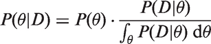
Usually the denominator is not analytically soluble, but since it is a constant of proportionality it follows that

The distribution
The MCMC approach has the useful property that it can be used to estimate missing values as well. The posterior distribution of the missing data can be considered in the same way as other unknown quantities. If

MCMC applied to the ESPON data set
Experimentation with the existing population time series suggests that some relatively simple models will yield reasonable predictions. We start with the quadratic Ordinary Least Squares regression model
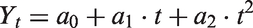
Here one uses the observed data to estimate the parameters

For our prior distributions, we make the following assumptions about the nature of the parameters. All of a0, a1 and a2 are drawn from a normal distribution, ρ from a beta distribution and
The series is modelled by sampling from a multivariate normal distribution, with a vector
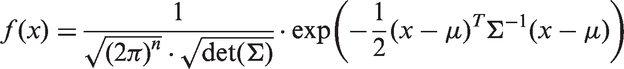
For this purpose, let us divide the time series into a sub-series of missing data points and a sub-series of present data points. Then we rearrange Σ according to this subdivision so that Σ looks as follows:
Finally let
As the missing data can be treated like a missing parameter in our MCMC process, it follows that the conditional distribution of the missing data given the present data depends on the joint distribution and the distribution of the present data, that is, if X denotes the random variable of the missing data and Y denotes the random variable of the present data, then
Eaton (1983) has shown that
Running the model
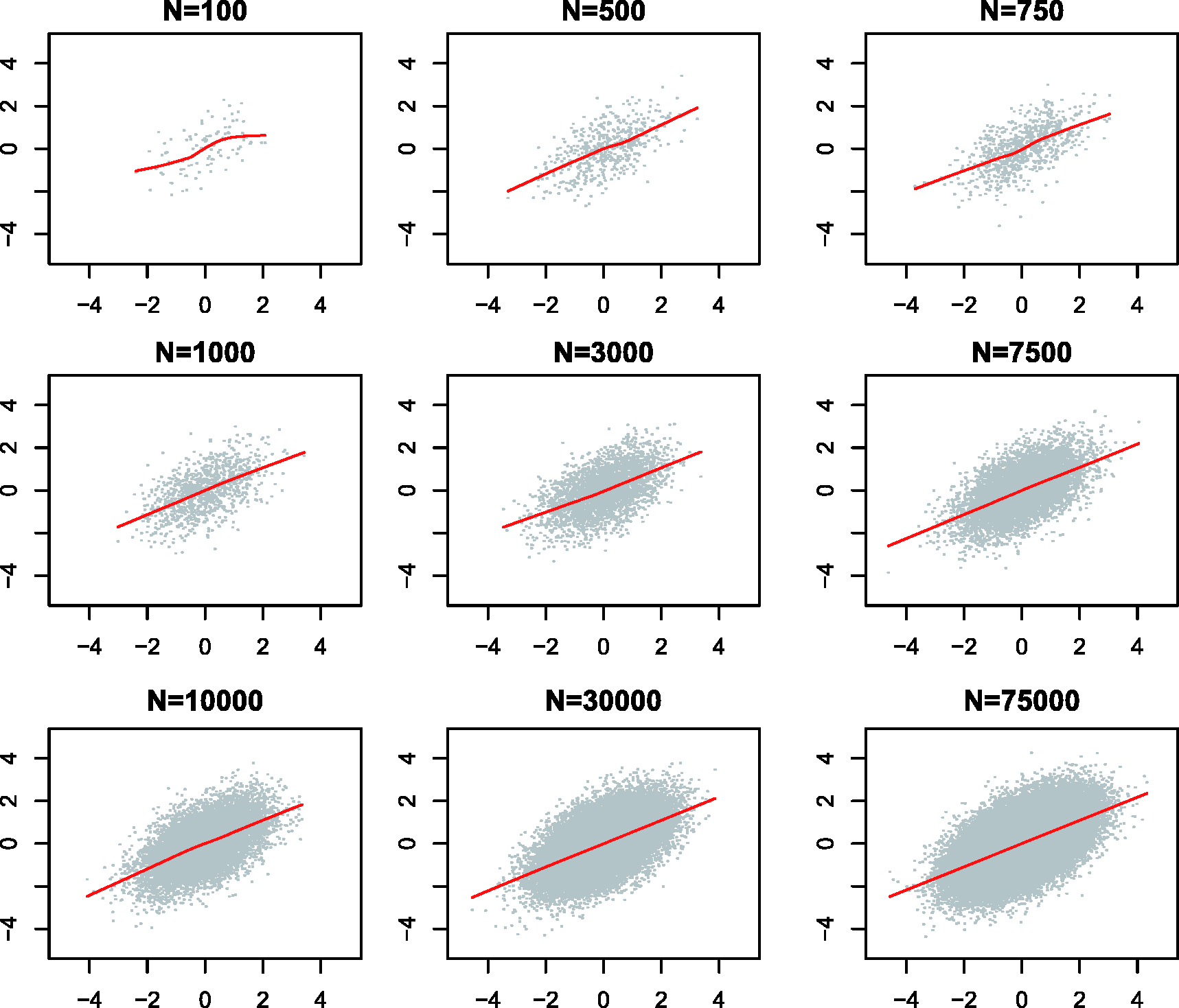
Recall that the parameter vectors in the Markov chain are approximately from the posterior distribution only after a sufficient number of iterations. In practice, every MCMC process starts with an initial burn-in phase. During the burn-in a certain number of iterations are performed, however the results are ignored and do not appear in the posterior distribution. This is to give the Markov chain ample time to get sufficiently close to its equilibrium distribution. Generally it is not clear how many iterations are sufficient. The danger of using too few burn-in iterations is that the posterior intervals are still too wide. Gelman and Rubin (1992) propose a convergence diagnostic. Figures 3 and 4 indicate how the uncertainty in the output decreases with an increasing number of iterations.
Normal distribution after a varying number N of iterations. Multivariate normal distribution after a varying number N of iterations.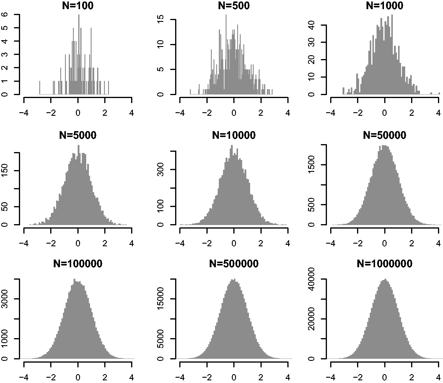
In the case of the population time series we started with an initial burn-in of 250,000 iterations. From then on every fifth iteration is sampled until 100,000 samples have been collected. The method of not sampling after every iteration step is called “thinning” and it is necessary as the result after an iteration step depends on the previous result. Thus by “thinning” the chain we get a little closer to obtaining independent identically distributed draws. Overall the estimation is then based on those 100,000 samples. Hence the estimated value is a distribution of possibilities.
Besides getting estimates for the parameters and the missing data we can also extract the highest posterior density from the set of samples. This is defined as the shortest possible interval enclosing
Ensuring spatial coherence
Recall that the ESPON data has a spatial component which comes from the NUTS hierarchy. All NUTS1, NUTS2 and NUTS3 regions are children, that is, they are part of a NUTS region of a higher level. Likewise NUTS0, NUTS1 and NUTS2 are parents, that is, they divide into NUTS regions of a lower level. In order for the database to be consistent we have to make sure that all observed and predicted values of the children add up to the value of their parent.
In the following, we describe how we ensure spatial coherence and how this procedure is consistent with our Bayesian framework. Note that observed values in the data set are real values while our predictions are sampled from simulations. In order to justify an approach that allows us to deal with both observed values and predicted values as if they belonged to the same class, we regard the observed values as being simulations from the limiting case of a normal distribution with an infinite precision, that is, a zero variance. Note that the precision τ controls the variability σ of the simulated distribution due to the relationship Increasing the precision τ simulates numbers closer and closer to the mean.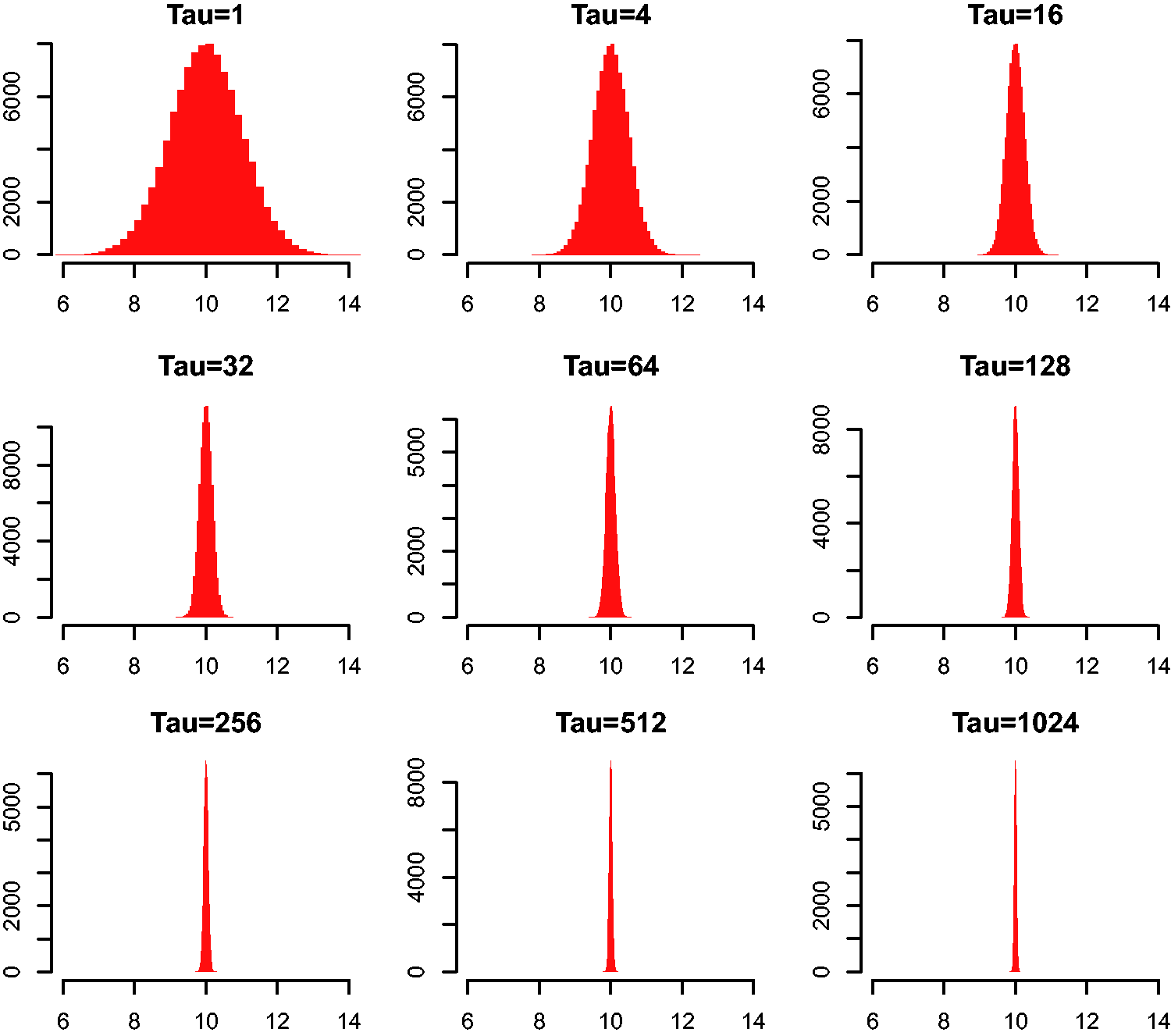
Ensuring spatial coherence is a top-down cross-sectional operation. First, we ensure spatial coherence between the NUTS0 region and all its NUTS1 region. That means for the country (NUTS0 region) under consideration we constrain the values of the NUTS1 regions which it contains. Next we ensure spatial coherence between each NUTS1 region and its containing NUTS2 regions, that is, for each NUTS1 region we constrain the values of the NUTS2 regions which it contains. Finally, we proceed the same way with each NUTS2 region and all its constituent NUTS3 regions.
Recall that we consider the NUTS hierarchy as a tree. Hence the same algorithm can be applied irrespective of the level we are at. Whether we ensure spatial coherence between the NUTS0 region and its containing NUTS1 regions or between a NUTS2 region and its containing NUTS3 regions the procedure remains the same and we describe it in the following:
Let A be a NUTSX region with value vA. The value vA is either an observed value or has been predicted using MCMC. In the latter case, the top-down component of our operation will already have ensured spatial coherence between A and its siblings and their parent region. Whatever the situation a finalised value vA exists. Also let

That means the proportion of
Software
Software for MCMC approaches has been, until recently, the province of the specialist. This altered with the release of BUGS (Bayesian inference Using Gibbs Sampling) (Lunn et al., 2009, 2012). BUGS has now been extended with a Windows interface (WinBUGS) and to handle spatial data (GeoBUGS). However, data preparation and post-modelling evaluation requires other software. The release of JAGS (Plummer, 2015) provides a further milestone. It offers a very similar facility to BUGS, but it is open source and may also be used in conjunction with the statistical programming language R via the rjags package. This offers R users the capability of fitting models using MCMC, while giving the power and flexibility of R, in order to prepare the data, and to provide extensive evaluation of the results in the R environment. Using JAGS, it is possible to obtain posterior distribution for the parameters and for the missing data. The R package has also been used to implement the data checking procedures.
Results
An Austrian example
In this section, we show the steps of our methodology by working through the available data of Austria. The indicator under consideration is the population figure. Austria has three NUTS1 regions, 3, 2 and 4 NUTS2 regions, respectively, and a total of 34 NUTS3 regions. From Figure 6, we see that population values are present for the entire time frame for all NUTS0, NUTS1 and NUTS2 regions, but are missing for all NUTS3 regions from 1990 to 2001 inclusive.
Austria – available population values: The diagram shows for which NUTS regions data are present or missing. It is also a heatmap of population totals, where colder colours in the spectrum represent lower populations and warmer colours represent larger populations.
Once the data has been collected from EUROSTAT and the National Statistics Office, the entire process of data completion comprises three stages. First, we check for values that are missing from the data but can be determined directly from other observed data points. Secondly, we predict all missing values using an MCMC estimation. Finally, the data is adjusted for spatial coherence.
In our case, the situation in which a parent is missing but all its children are known, or the parent and all but one of its children are known does not occur. Therefore step one of our process is not necessary or, if performed, will not improve the state of the data.
Figure 6 shows a heatmap of the population totals. The colder colours in the spectrum represent lower populations and the warmer colours represent larger populations. In general, the population for AT and its NUTS1 regions have grown over the 22 year time period from 1990 to 2011. However, the trajectory of some individual zones has been different: that for AT21 had considerable growth to the mid 1990s, followed by a gradual decline over the rest of the time period.
In the next stage, we run the MCMC algorithm to estimate all missing population values. One needs to be aware that for all 34 NUTS3 regions a time frame of 12 years was missing. This represents approximately 55% of the NUTS3 data. This means that at best, we have 45% of the NUTS3 data as evidence on which to base the retropolations, although we also have 100% of the NUTS2 data to act as a constraint. The first heatmap in Figure 7 shows the unadjusted NUTS3 estimates as derived from the MCMC algorithm.
Austria – unadjusted population estimates (left) and spatially coherent population estimates (right).
In the last stage, we adjust the data for spatial coherence. For this an algorithm runs from top to bottom through each parent region and adjusts all estimated values on a pro-rata basis. As the children of all parents at the NUTS0 and NUTS1 level are observed no adjustment is needed here. Finally for every parent at the NUTS2 level from 1990 to 2001 an adjustment takes place. The second heatmap in Figure 7 shows the spatially coherent population figures.
Let us now take a closer look at the NUTS2 region AT21 (Kärnten) and its three NUTS3 children AT211 (Klagenfurt-Villach), AT212 (Oberkärnten) and AT213 (Unterkärnten). For each region, we use the available data for the years 2002–2011 inclusive to derive estimates from the MCMC algorithm for the missing years 1990–2001 inclusive. Finally, we use the available totals of AT21 for the years 1990–2001 inclusive to enforce spatial coherence among the MCMC estimates of AT211, AT212 and AT213. Figure 8 shows the available data, the unadjusted estimates and the spatially coherent estimations. Finally note that even though the jump from 1990 to 1991 looks dramatic it only represents a growth of 0.5%.
Austria – estimates for AT211, AT212 and AT213 for the years 1990–2001 inclusive. The grey dots represent the available data, the dotted line shows the estimated population from the MCMC algorithm and the uninterrupted line shows the spatially coherent estimates.
Assessment of the methodology
Let us assess the performance of our methodology by estimating population figures which we already know. As mentioned above the values for all three NUTS1 regions of Austria are given for all the years 1990–2011. In the following, we assume the six years from 1990 to 1995 to be missing. We run the estimation process for those values based on the present NUTS1 figures for the years 1996–2011 and enforce spatial coherence with respect to the given NUTS0 figures for the years 1990–1995.
The first figures in Figures 9 to 11, respectively, show the imputation process for the three NUTS1 regions AT1, AT2 and AT3, respectively. We see in all three cases that the estimated trend diverges very quickly from the actual values during the years 1995 back to 1990. For instance for both AT1 and AT3, the estimated value for 1990 is off by nearly 100,000 people. The estimated trend for AT2 during the years 1990–1995 is downwards, while in reality the trend is upwards during that period.
Imputed and spatially adjusted population figures for Austrian NUTS1 region AT1. Imputed and spatially adjusted population figures for Austrian NUTS1 region AT2. Imputed and spatially adjusted population figures for Austrian NUTS1 region AT3.
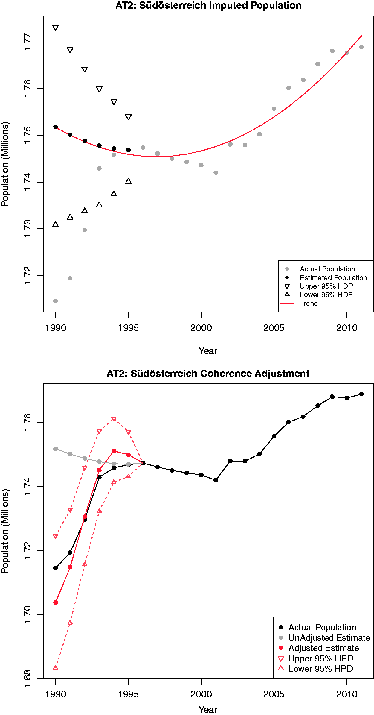
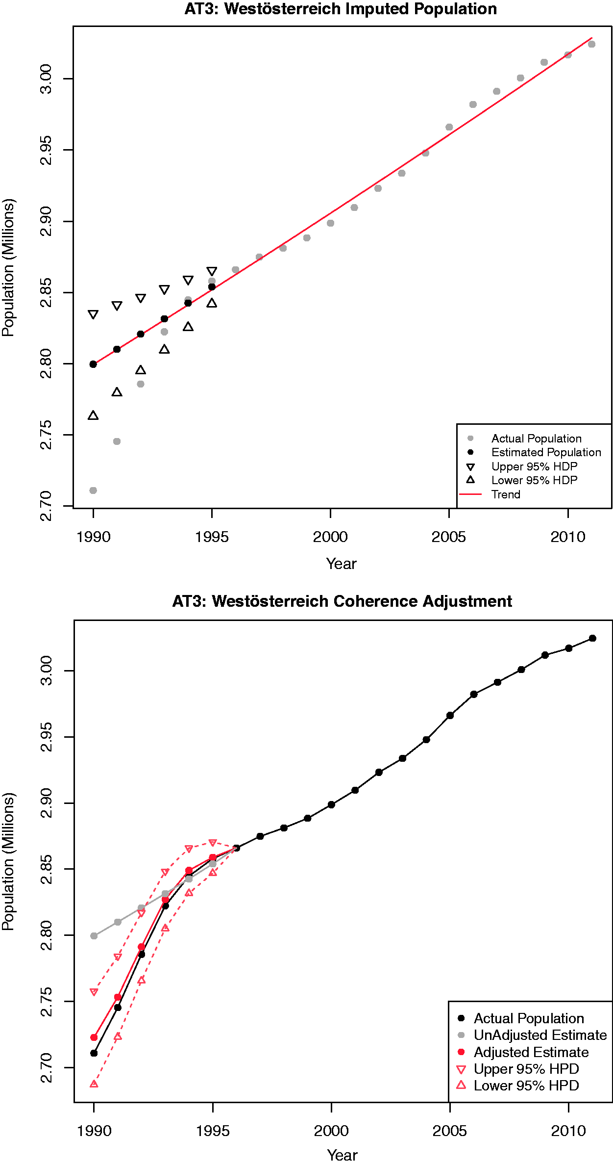
Next we exploited the knowledge which comes from the present NUTS0 values for the years 1990–1995. We adjust the estimated values to ensure spatial coherence with respect to the NUTS0 region, that means, for each year we ensure that the sum of the estimates for AT1, AT2 and AT3 adds up to the present value for the entire country. Applying a pro-rata we derive at the new, adjusted estimates as given by the second figures in Figures 9 to 11, respectively. Note how after the process of ensuring spatial coherence, the estimated values are much closer to the actual values. Also the actual trend in the data is captured more realistically.
Scalability
The question of the practicability of the approach, given the nature of MCMC estimation should be considered. The ESPON series are short run – in the case of the population data, we have no more than 25 observations. In the worst case all 25 observations are missing, and no amount of MCMC will recreate the data. The time required depends on (a) the speed of the processor, (b) the number of burn-in cycles and (c) the number of estimation cycles. Counter-intuitively, the more data that is present, the longer the estimation process takes. Figure 12 depicts the relationship between the proportion of missing data and the time required to estimation the missing data in the series.
Scalability of MCMC estimation.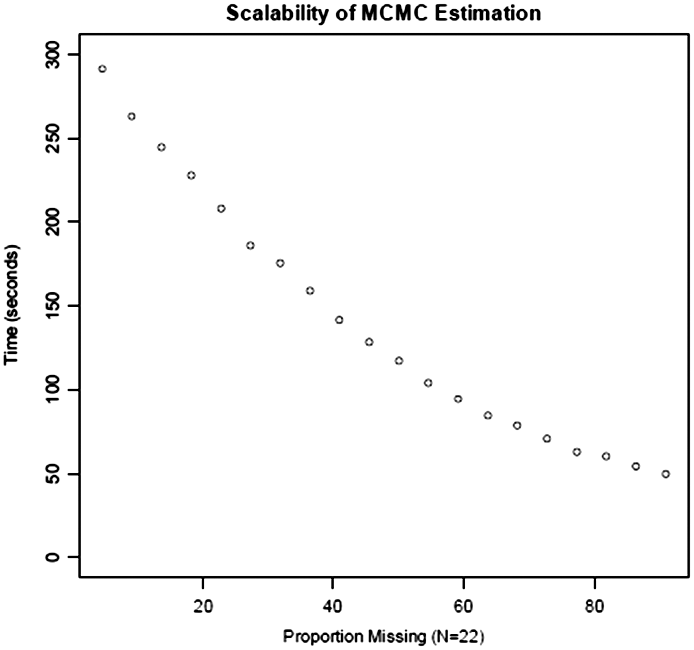
In the population series, about 28% of the data was missing. The MCMC estimation for the entire dataset, that is, all missing NUTS0, NUTS1, NUTS2 and NUTS3 regions, took about 60 hours on a quad core 3.16 GHz Intel Xeon processor running Windows XP Professional. This would equate to about 35 hours on a laptop running Windows 7 Professional on a 2.80 GHz Intel Core i7-2640 M processor. In comparison, the adjustment to spatial coherence was completed in a total of 13 seconds.
Other series in the dataset
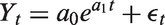
The process presented in this paper is equally applicable to any other indicator of interest in the database, such as employment or GDP. In fact, the completed time series for one indicator may be used in the completion of another. For instance, the prediction of the GDP series might include population and unemployment as covariates, that is, we use the model

Conclusions
The production of a coherent and reliable space-time socio-economic indicator was the goal of the activity described in this paper, using a robust approach to imputing missing data in a consistent way given the characteristics of the dataset. This has been achieved using a valid statistical model which also satisfies the spatial constraints of the problem by ensuring that the summed values of the nested regions equal the value of the corresponding parent region.
Our Bayesian approach to the problem does not just fill the holes in the time series but also produces accompanying error bounds, thus giving an indication of the confidence level in the imputation. This further strengthens the results. Furthermore our method is very flexible as it is independent of the nature of the data and works irrespective of the chosen model. The entire algorithm has been implemented using open source software, R and JAGS, making it an accessible tool for other users as well as ensuring the reproducibility of any results.
This provides but one small element in the set of activities leading to the wider goals of EU territorial cohesion. It also provides the basis for further work on other space-time socio-economic components of the ESPON database, including births, deaths, employment and gross domestic product. However, it should be noted that as a methodology it provides a general approach to the imputation of missing data in space-time data series. As such it can be employed for data imputation in short run time series, which also form part of a spatial hierarchy. As such it acts as a suitable tool for the production of evidence to support policy creation, evaluation, implementation and monitoring.
Footnotes
Acknowledgements
Text and maps stemming from research projects under the ESPON Programme presented here do not necessarily reflect the opinion of the ESPON Monitoring Committee.
Declaration of conflicting interests
The author(s) declared no potential conflicts of interest with respect to the research, authorship, and/or publication of this article.
Funding
The author(s) disclosed receipt of the following financial support for the research, authorship, and/or publication of this article: The authors gratefully acknowledge support from the ESPON Programme under contract 114/2011.