
Abstract
The ‘at-risk-of-poverty’ rate is the most widely recognised indicator of income poverty. Its principal advantage is that it is relatively straightforward to define and (given appropriate data) to calculate. National at-risk-of-poverty rates play a key role in monitoring EU2020 objectives relating to combating poverty. Regional patterns of poverty have the potential to deepen our understanding of processes of impoverishment and differentiation, and how they can be more effectively addressed by policy. Estimating regional poverty rates, and especially producing a European map, is a challenging task, given current data resources. This paper begins by placing the at-risk-of-poverty rate within the wider conceptual context relating to poverty, social exclusion and deprivation. It then provides an account of an exercise to map at-risk-of-poverty rates at NUTS 3 across 20 European countries. Together with data derived from national registers (where available) and more direct apportionment methods, coverage of most of Western Europe is achieved. The patterns revealed are described, and generalisations, which serve as pointers to further research on the processes responsible, are derived. The paper concludes with some reflections on the value of regional at-risk-of-poverty rates in advancing our understanding of the distribution and causes of poverty, and hence appropriate interventions to ameliorate it.
Annual income twenty pounds, annual expenditure nineteen pounds nineteen and six, result happiness. Annual income twenty pounds, annual expenditure twenty pounds nought and six, result misery. – Mr Mcawber in David Copperfield by Charles Dickens
Introduction
This paper is concerned with indicators and mapping of income poverty, their capacity to clarify our understanding of spatial patterns and processes of disadvantage, and their potential role in policy targeting and monitoring.
It is important, at the outset, to distinguish income poverty from several closely related phenomena with which it may sometimes be confused. Income poverty is measured solely in terms of the disposable income available to the household or individual. It does not consider non-pecuniary issues which are commonly associated with the broader concepts of poverty, deprivation (Townsend, 1987) and social exclusion (Talbot et al., 2012). Neither is expenditure, or the various different calls on income which vary with location, personal circumstances and characteristics, taken into account.
Analysis has shown that households and individuals affected by income poverty do not always coincide with those who experience material deprivation (inability to purchase basic goods and services) or other less tangible forms of poverty (Whelan et al., 2001, 2002). Some households are poorer, or more deprived than their income would lead us to expect, and vice versa. For this reason indicators of income poverty are sometimes described as ‘indirect’ measures, whilst those which measure outcomes in terms of deprivation are termed ‘direct’ (Ringen, 1988).
So why are indirect indicators of income poverty, such as the at-risk-of-poverty (ARoP) rate, or child poverty rates, so commonly used as a basis for policy decisions? The answer is simply that, at a national level, they are relatively easy to estimate from existing data sources, either income registers covering 100% of the population, or, more commonly, national or European sample surveys, such as the EU Survey of Income and Living Conditions (EU-SILC). 1
Poverty is a spatially heterogeneous phenomenon, and poverty rates can vary widely over space. The study of geographical inequalities therefore is a very important dimension of poverty analysis. Regional or local policies require a better understanding of patterns of poverty at an appropriate scale. Regional differentiations of poverty risk should be taken into serious consideration in policy making and policy implementation. Poverty might have strong local characteristics and this is something that should be carefully examined by policy makers because, sometimes, targeted policies might be more effective than general interventions. National level indicators are useful to monitor the global trends but disaggregated information for lower geographical (administrative) areas is probably more useful for policy makers. From this perspective, poverty maps that provide a description of the spatial distribution of welfare and poverty within a country at different spatial levels and can be used to investigate the relationship between poverty and other economic, social and geographic factors, are a useful tool for analysis and policy making. As Crow et al. (2009) suggest visualisation matters in the study of inequality and poverty since maps (and graphs) might present powerful stories about progress, social change and development.
Where the source is register data it should be a relatively simple matter to disaggregate national data and generate ARoP rate maps. More commonly, where the data source is a national survey, sampling regimes are unlikely to be robust enough at a local or regional level, and some form of modelling or apportionment will be required. This paper provides an account of an attempt to compile a map of ARoP rates for more than 1200 NUTS 3 regions 2 across 20 European Countries. We believe this to be the first successful attempt to provide a European-wide map of income poverty at the NUTS 3 region level. 3 Our work hopefully provides better support to the design of regional poverty alleviation strategies than previous, more aggregate, maps for NUTS 2 or NUTS 1 regions (CEC, 2005; Verma et al., 2006), which can hide considerable local variation in levels of income poverty.
The paper has the following structure: the next section provides the policy context for the analysis undertaken, while ‘The ARoP rate as an indicator’ section offers a brief discussion of the validity of the ARoP rate as an indicator of poverty. The following section discusses the empirical methodologies used and their main strengths and disadvantages. The subsequent section presents the composite poverty map for European NUTS 3 regions and discusses some of the key regional patterns and processes arising from the data. The final section summarises the main conclusions and recommendations for European wide research in the topic.
Policy context for the analysis
The EU has no specific, dedicated, Community policy to address poverty and social exclusion (for an extensive discussion about poverty issues in the EU see Betti et al., 2012; Fahey, 2007; Marlier and Atkinson, 2010; Whelan and Maıtre, 2010). Whilst a number of community policies, especially Cohesion policy, undoubtedly have some impact, poverty and social exclusion are mainly tackled through interventions organised at the Member State level. Since 2000 these have been ‘orchestrated’ through a procedure known as the Open Method of Coordination, within the structures provided first by the (2000–10) Lisbon Objectives (CEC, 2004), and more recently (2010–20) by EU2020 (CEC, 2010). At the Lisbon meeting in 2000, the European Council set the strategic goal of ‘greater social cohesion’ and committed to take steps ‘to make a decisive impact on the eradication of poverty’. This strategy put poverty and social exclusion at the heart of EU social policy and led to the adoption in 2001 of the Laeken social indicators including, among others, poverty indicators. Tackling poverty is also one of the objectives of the Europe 2020 Strategy. The key poverty and social exclusion target in the context of EU2020 is to lift 20 million people out of poverty and social exclusion by the year 2020 (Eurostat, 2004, 2005, 2007, 2012).
The EU2020 target has been operationalised in terms of three indicators:
The number of persons at risk of poverty, i.e. the number of persons in households whose disposable income is less than 60% of the national median; The number of persons not able to afford four of out of nine items indicative of material deprivation; The number of persons living in households where adults (together) work less than 20% of a full time year.
The three indicators above, added together but avoiding ‘double counting’ of individuals constitute the means of monitoring the EU2020 goal in aggregate terms, though differences in the way in which Member States define their targets mean that it cannot be reconciled directly with the 28 national objectives. 4
Data requirements for the three EU2020 indicators are mainly satisfied from the EU-SILC. Although, in the context of the EU2020 targets, monitoring is only required at Member State level, Eurostat publishes NUTS 2 data for the three constituent indicators. Coverage varies from country to country, some at NUTS 2, some NUTS 1 and some for the whole country (NUTS 0). In most countries, the most recent data currently relates to 2012 (Copus, 2014).
Within the context of the 2014–20 programme of the European Structural and Investment Funds, some opportunities exist for regionally targeted poverty alleviation measures. This explains current interest in estimating and mapping regional ARoP rates.
The ARoP rate as an indicator
The ARoP rate is defined as the percentage of persons in households whose equivalised
5
disposable income is less than 60% of the national median. This indicator has some rather unusual characteristics, which make it rather tricky to estimate and to interpret. It is both an indicator of the level of income and its distribution. The relative strength of these two sources of variation depends upon the choice of ‘benchmark’ to define the ‘60%’ of median disposable income. It is conventional to use the national median as the benchmark. This means that regional ARoP rates can be quite closely correlated with their median disposable income levels. If each region had its own ARoP benchmark, based upon its regional median income, variation in the ARoP would be entirely a function of the local income distribution – or degree of inequity (Eurostat, 2004). To express it another way the geography of ARoP rates is a complex combination of variations in income levels and distributions. In terms of Figure 1, regional rates vary partly as a result of shifts in the income distribution curve to the left or right, and partly due to changes in the shape of the distribution.
The ARoP rate. Source: Own elaboration.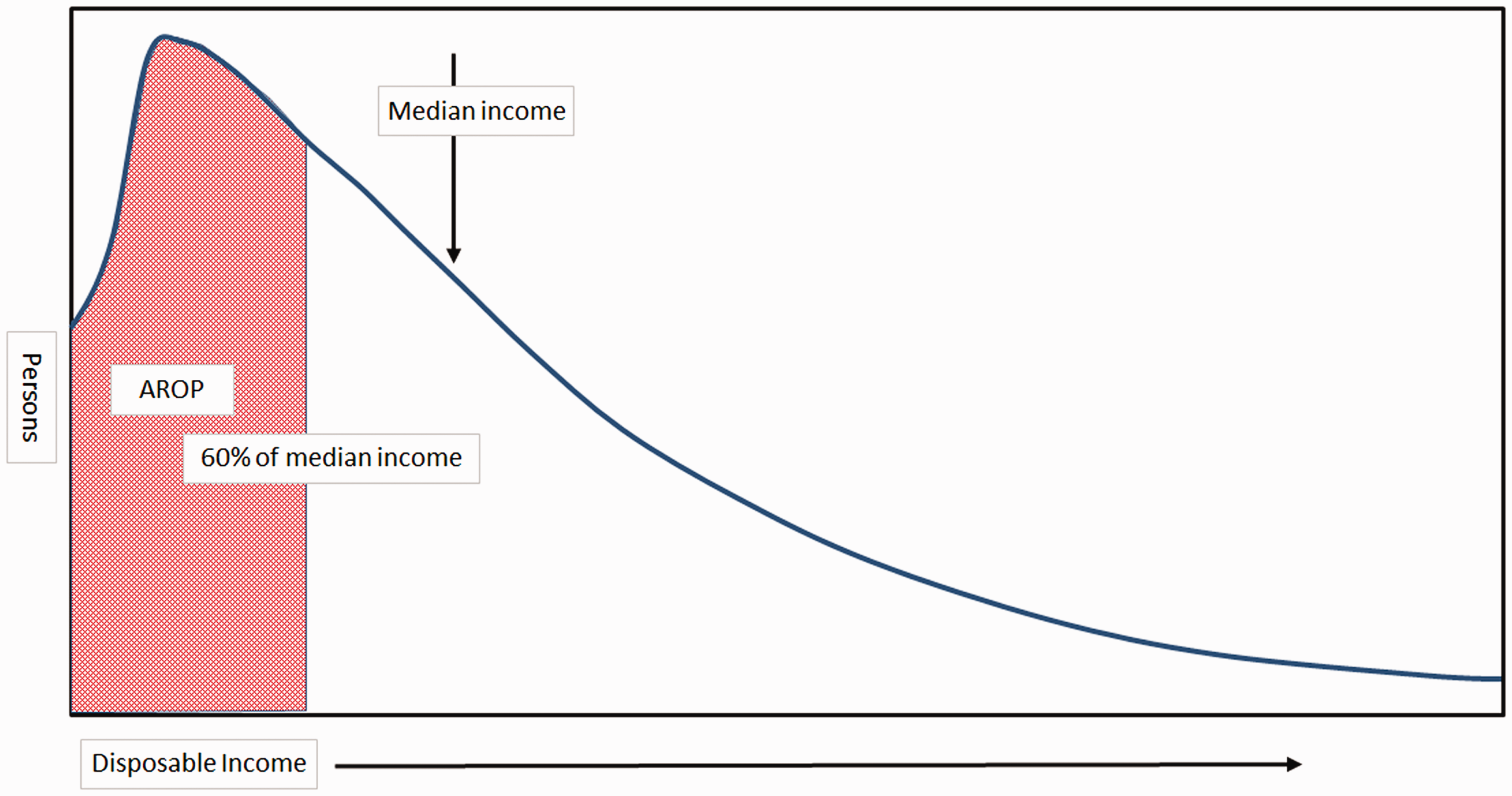
As we have already mentioned, it is important to recognise the fact that measures related to disposable income may not identify all individuals and groups who are experiencing poverty even in a narrow financial sense. Some authors favour the adjustment of ARoP rates by excluding housing costs (rent and mortgage interest) from disposable income (e.g. Aaberg et al., 2008; Pittau et al., 2011). The rationale for this change is that housing costs are the most significant component of regional differences in the cost of living within countries, and that excluding them is a way to ‘level the playing field’ between the regions. Analysis by the European Commission (CEC, no date) suggested that this adjustment would (on average) increase the ARoP rate (from 17 to 21% for the EU27), affecting some Member States more than others, and reducing the difference between urban and rural areas (Dijkstra, 2012, personal communication).
However, recent research in the UK suggests that housing costs are not the only form of expenditure which varies substantially between regions (Hirsch et al., 2013). A broad range of consumer goods, food and fuels all tend to be more expensive in remote rural or island areas. In addition, sparsity and climate may impact upon the average expenditure profile of families in these areas, increasing the travel cost of daily life, and the cost of heating the home. However, this line of research has yet to progress beyond case studies into the field of regional indicators.
NUTS 3 estimation methodology – A pragmatic choice determined by data availability
The TiPSE project, upon which this paper is based, was tasked with producing a NUTS 3 map of ARoP rates for all countries within the ESPON programme area, 6 except the countries of Central and Eastern Europe which acceded in 2004 and 2007. The latter are the subject of a preceding project, conducted by the World Bank (WB).
The initial intention was to follow, in all countries, the World Bank’s PovMap (WBPM) methodology, 7 and associated software, which generates NUTS 3 estimates of the ARoP rate through a regression modelling technique, combining information from EU-SILC and 2011 Population Census microdata (Elbers et al., 2002, 2005). This method is based heavily on the literature on Small Area Estimation techniques. Small area estimation techniques are one methodology that can be used to provide reliable information about poverty rates (Haslett and Jones, 2010). However, it was quickly realised that in certain countries, notably the Nordic states and the Netherlands, estimation was unnecessary, since ARoP rates could simply be derived from register data. Since these are derived from full population data, the issues of sampling and statistical modelling errors do not arise.
In a few countries national statistical agencies have produced their own ‘official’ estimates of regional ARoP rates. These were considered a more reliable option than other estimation strategies available to the TiPSE research team, since they are often based on data sources not publically available. However, careful scrutiny of methodology and definitions was necessary in order to ensure an acceptable degree of comparability with the ARoP rates for other European countries.
Where register data were not available, and estimation had not been carried out by national statistical authorities, the preferred estimation procedure was the WBPM. However, PovMap is rather demanding in terms of data. There are two principal technical constraints:
Firstly, the model requires that the EU-SILC microdata contain regional identifiers which allow the sample to be divided into a number of geographic ‘clusters’, for each of which the relationship between poverty and a set of socio-economic covariates is derived through regression modelling. These clusters must be intermediate between the whole country and the level at which the ARoP rate estimates are required (in this case NUTS 3). Effectively this means that the EU-SILC microdata need to contain either NUTS 2 or NUTS 1 identifiers. In a number of EU Member States the sample size is insufficient, and the regional identifiers are suppressed.
Secondly, it is necessary to have a sufficient number of indicators which are common to both the EU-SILC and the Census microdata. This is required because the parameters obtained from the income regression model estimated using EU-SILC data are applied to the more spatially disaggregated Census data to produce regional measures of income and ARoP rates (in our case for NUTS 3). A high level of compatibility, both in terms of definition, and (because many variables are categorical rather than continuous) in terms of classes, is required.
In addition to these technical constraints, the timing of the project (2012–14), and delays in the release of 2011 Census microdata, proved serious limitations to the research. Indeed the switch from conventional census to register-based databases in many European countries may mean that microdata samples are unlikely to become available at all. As a result of these combined difficulties, PovMap modelling was only possible in a handful of countries.
The next-best option for estimating NUTS 3 ARoP rates would be regression models based upon aggregate (rather than individual or household) data (Copus and Coombes, 2014). These too combine EU-SILC and Census data, but using regional aggregate data rather than microdata. Again it is necessary that the SILC data contain NUTS 2 or NUTS 1 identifiers, in order to permit modelling at one of these aggregate levels. In this case, an additional constraint is added; there must be a sufficient number of cluster-level regions to allow a statistically significant regression model to be achieved. There are unfortunately a number of European countries in which there are less than 10 NUTS 2 regions. The requirement for consistent definitions and categories is also important here, though the availability of 2011 Census data is less of a limitation, since regional data have generally become available earlier than microdata. In practice, the small number of NUTS 2 regions was the main barrier to implementation of such ‘area-based’ models, which again proved feasible in only a small number of countries.
Where none of the above options were available recourse to univariate apportionment procedures was necessary. The usage of such an apportionment method assumes that there is a close dependency between the spatial distribution of one dimension represented by a single indicator and the distribution of the targeted ARoP rate. The correlation between these two distributions must be high. In the case of a positive correlation, a high value of the underlying variable means a high number for the ARoP rate and vice versa. Therefore, the variable used must be carefully selected. When interpreting the output of the method it is also always necessary to keep in mind that it shows mainly the distribution of the one-dimensional indicator, projected to the ARoP rate. To calculate the ARoP rate over NUTS 3 regions of one country, the average national (NUTS 0) ARoP rate, extracted from EU-SILC, is multiplied by the z-standardised value of the selected indicator. This method leads at first to an inconsistency in comparison to probably available EU-SILC-based ARoP rates on NUTS 1 or NUTS 2. To overcome this, the calculated NUTS 3 rates may be adjusted to the available higher level. This method was used in Belgium, Spain, Portugal and Switzerland, where the number of NUTS 1 and NUTS 2 regions is too few to allow a more sophisticated regression model and availability of proxy indicators relatively poor.
Overview of approaches implemented.

ABM: area-based model; APPT: univariate apportionment; EUSILC: European Union Statistics on Income and Living Conditions; NSI: estimates produced by the National Statistical Institute; REG: register data; WBPM: World Bank PovMap.
In addition to the data listed in Table 1, the maps and analysis presented in this paper incorporate (WBPM) ARoP rate estimates for Hungary, Latvia, Romania, Slovakia and Slovenia, generously made available to us by DG Regio. In those countries for which no NUTS 3 estimates are available, Eurostat data 9 at the lowest NUTS level available was used to complete the maps and to populate the dataset.
Strengths and weaknesses of the alternative approaches to the estimation of regional ARoP rates
As discussed above, the choice of approach used to estimate ARoP rates for NUTS 3 regions was constrained by issues of data availability. Ideally, we would like to have used estimates produced by each country’s respective national statistics authority, either directly from register-based data or indirectly from national surveys or the combination of national surveys with Census data. Where this approach was not possible we had to carry out some form of estimation (in order of preference):
World Bank PovMap (WBPM); ABM; Univariate apportionment (APPT).
The main advantages of the WB poverty mapping methodology (WBPM), compared to the simpler ABM and univariate apportionment (APPT) include:
Better representation of the multi-dimension nature of poverty through the inclusion of multiple proxy variables (for welfare) simultaneously; Availability of measures of the statistical precision (i.e. confidence intervals) of the indicators of poverty produced; Ability to compute different measures of poverty (e.g. headcount index, poverty gap index, poverty severity index) and inequality (e.g. gini coefficient, generalised entropy measures, Atkinson’s inequality measures).
The WBPM methodology also has weaknesses, which are common to any technique based on statistical regression models. These weaknesses arise from small sample size, poor model specification and the inappropriate choice of statistical estimator. All three issues can affect the quality of the parameters obtained from the income models estimated in PovMap to generate estimates of indicators of income poverty.
The principal reason for using the ABM regression method, instead of the WBPM method, was the unavailability of appropriate microdata. Even if Census microdata do exist, the challenges involved in reconciling the Census microdata variables with the EU-SILC microdata variables may be too great. With the ABM approach the covariates at NUTS 2 and NUTS 3 may both be derived from the Census, and the problem of matching their definitions does not arise. On the down side, the ABM approach is vulnerable to the ecological fallacy. In other words, instead of estimating relationships between disposable income and socio-economic covariates at a household level, it does so on the basis of NUTS 2 regional averages. The latter may mask substantial intra-regional differences, which could potentially distort the estimates at NUTS 3. A further disadvantage (shared with the univariate apportionment method) is that the definition of the ARoP rate becomes fixed by the rates available at NUTS 2. It is not possible (as in the case of the WBPM approach) to carry out sensitivity analysis with different poverty lines.
Where the number of regions available to implement the ABM methodology is small, we had to adopt a simpler and less data demanding alternative based on direct univariate apportionment to produce ARoP rates. The main advantage of the APPT approach is its simplicity. The main disadvantage is that the weights used in the apportionment may not correlate well with the distribution of income poverty rates within the sub-populations of interest (in our case NUTS 3 regions), giving rise to measurement error in the estimates of the ARoP rate. As with the ABM approach, it is not possible to carry out sensitivity analysis with different poverty lines.
A consequence of the necessary adoption of different methodologies to estimate NUTS 3 ARoP rates is a limited ability to make the rates more comparable between countries. This requires careful consideration and interpretation of the composite European map of NUTS 3 ARoP rates, presented in the following section. There are two elements to the comparability issue:
The incorporation of national poverty lines. Clearly the median household income of some countries in the south and east of Europe is very much lower than those of the centre and north-west. Sadly, there is no way to implement a common poverty line. However, some simple adjustments can be made, which to some extent at least shed light upon the implications. One perspective on this would be to view the map of ARoP rates (Figure 2) as primarily showing patterns of the dispersion of income, since differences in level are to some extent subsumed by the national poverty lines. In effect it is closer to a map of degrees of regional inequality, rather than of differences in levels of income. Careful consideration should be given to the implications of this for the potential use of the map in policy targeting. Differences in estimation error, due to the different approaches used. Only the WBPM approach allows for variance estimation. These are available for United Kingdom, Greece and Austria (where the WBPM approach was implemented) on request from the authors. With respect to the other approaches it is still important to recognise estimation error as a constraint to comparability between countries.
NUTS 3 at risk of poverty rates: unadjusted.

Although due regard should be paid to the above cautions the composite map presented below is nevertheless of considerable interest as the best approximation to Europe-wide NUTS 3 regional variation in the ARoP rate with currently available data.
The resulting poverty maps
Figure 2 shows all the NUTS 3 ARoP rates estimated or collected by the TiPSE research team. As already explained, each country has a different poverty threshold, depending upon the distribution of household disposable income across its population. These range from €20,362 in Switzerland to €5,520 in Greece. From one perspective this could be said to be justified by differences in the cost of living, and by different expectations or perceptions of poverty. Nevertheless, it seems problematic that such differences take place abruptly along national borders, and either the map must be carefully interpreted with this in mind, or some form of adjustment must be attempted.
Taking the first of these options, the pattern revealed by Figure 2 is mostly quite reassuring. The highest rates of poverty are in Romania, Bulgaria, Eastern Poland, Eastern Germany, the Baltic States, Southern Spain, Southern Italy, Greece and Turkey, whilst the lowest rates are generally found in Northern Italy, Austria, Southern Germany, Netherlands the South of England, Norway, Southern Sweden and Iceland.
In Figure 3 the ARoP rates are shown as within-country-quintiles. The darkest greys pick out those regions within the highest 20% in each country, whilst the regions with the lightest shading are those in the 20% of regions with the lowest ARoP rates. In this map broad macro-regional disparities are ‘downplayed’ and more localised variation is emphasised. The pattern reveals a tendency for lower ARoP rates in the vicinity of capitals and other large cities (but not necessarily in the cities themselves, if tightly bounded), and relatively high rates of income poverty in remoter regions (such as Eastern Romania and Poland, Eastern Turkey, the Southern parts of Italy, Greece, France and Spain, South-West Ireland, West Wales, Western Scotland, Eastern Germany, Northern Sweden and Eastern Finland). The area along the Franco-Belgian border and the North-East coast of the Netherlands also show up as having relatively high rates of income poverty.
NUTS 3 at-risk-of-poverty rates: national quintiles.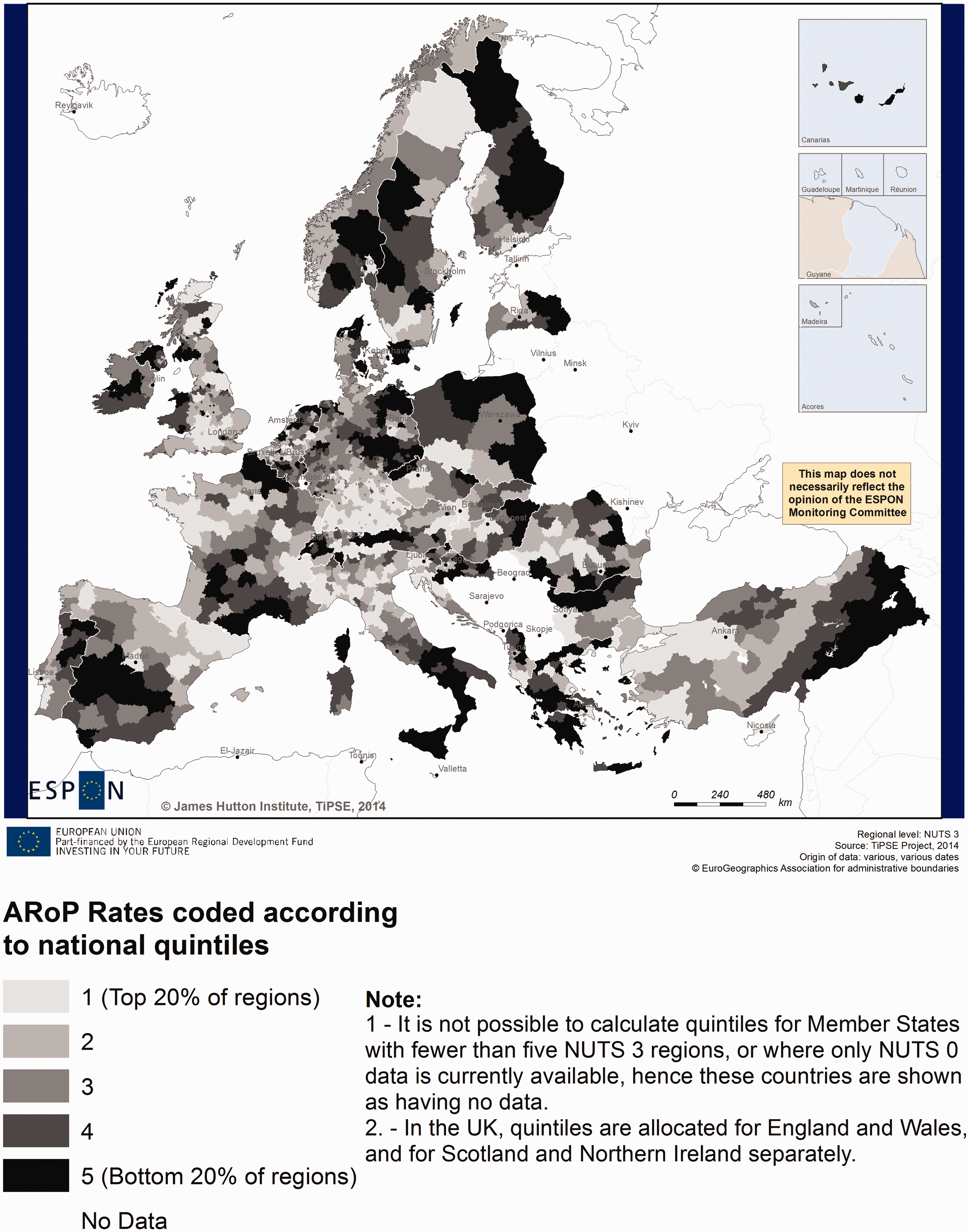
Figure 4 shows the same ARoP data, but this time expressed as an index of the national mean. The difference between this approach and the previous map is that the index reflects the scale/degree of the disparity between each region and the national mean, a metric which is to some extent lost in the quintile approach. Figure 4 therefore enables us to pick out the more extreme values, both positive and negative. Some of these reinforce the generalisations derived from Figure 3 (e.g. low rates around capital cities, high rates in Southern Italy and Spain). Others are less expected, such as the low rates of poverty along the border between Spain and France.
NUTS 3 at risk of poverty rates: national average = 100.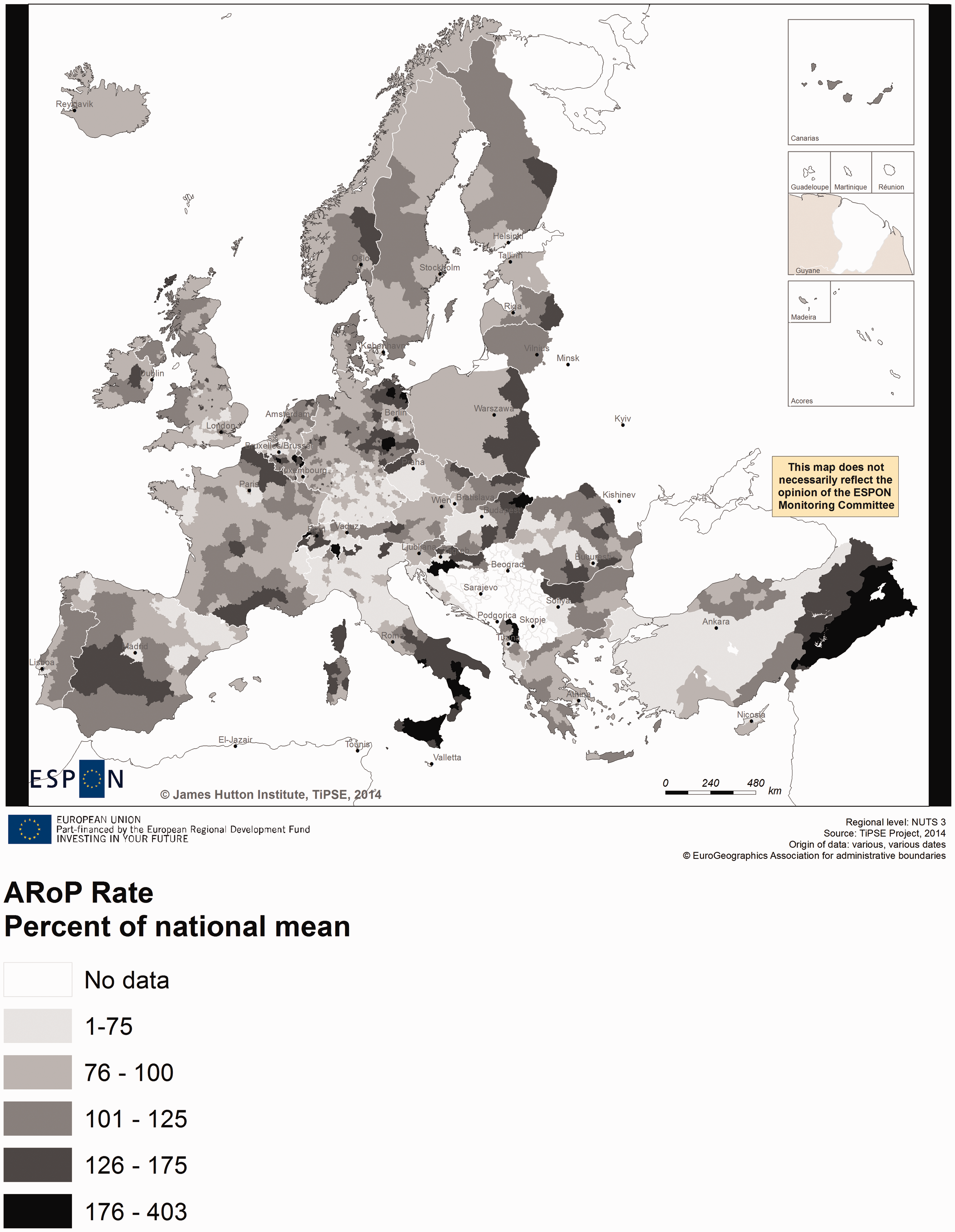
What can the regional ARoP rates tell us about patterns of poverty in relation to different kinds of region?
The above maps and commentary provide some initial first impressions of the spatial variation of income poverty at the NUTS 3 level. However, they do not take us very far in terms of developing an explanation of the causes of regional differentiation in income poverty. One simple way to begin to shed light upon this is to use regional typologies to explore how ARoP rates vary in different kinds of region, using a series of simple bar charts, which present ARoP rates averaged across each type of region within each country. This approach both avoids including data from countries in which a typology is not relevant (such as island regions in Austria), and means that data from different countries (with different poverty lines) are kept separate.
In this section, we describe how poverty rates vary between rural and urban regions, and between island and mainland regions. Typologies (all derived from the ESPON programme 10 ) relating to metropolitan regions, border regions, mountain regions, coastal regions and regions in industrial transition are included in the TiPSE project Final Report (Copus, 2014), but will not be reported in detail here, since the interpretation of the graphs is less clear cut.
The first typology (Figure 5) is the classification of NUTS 3 regions by At risk of poverty by urban–rural type, selected countries.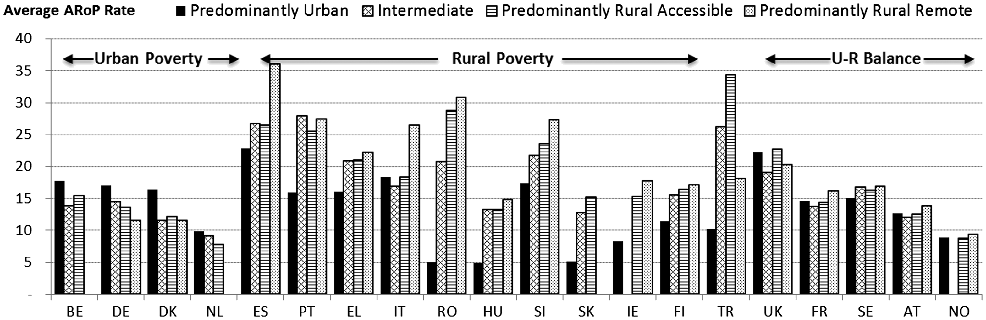
Figure 5 shows that there are some quite substantial differences between ARoP rates across this typology. Three broad groups of countries emerge. In four central countries (Belgium, Germany, Denmark and Netherlands) income poverty rates are higher in urban areas than in intermediate or rural areas. In a further 10 countries, income poverty rates are higher in rural and/or intermediate regions. The strongest associations with rurality are in the Mediterranean countries (Spain, Portugal, Greece and Italy), and in former socialist countries (Romania, Hungary). In Turkey accessible rural areas (mostly along the Eastern border) exhibit the highest poverty rates. In the final group (UK, France, Sweden, Austria and Norway), poverty rates seem less affected by rural–urban differences.
In some national contexts, NUTS 3 is too large a scale to pick up the role of insularity. Most islands are subsumed within larger regions which are predominantly ‘mainland’. Nevertheless, in Italy, Spain, Greece and France (Figure 6) island regions have significantly higher poverty rates. In Sweden, UK and Denmark island and mainland rates are almost identical. The remaining two countries, Portugal and Finland can be seen as special cases, due to the relatively low rates in Madeira (the only Portuguese island region for which there is data), and in Finnish Åland.
At risk of poverty rate, island and mainland regions.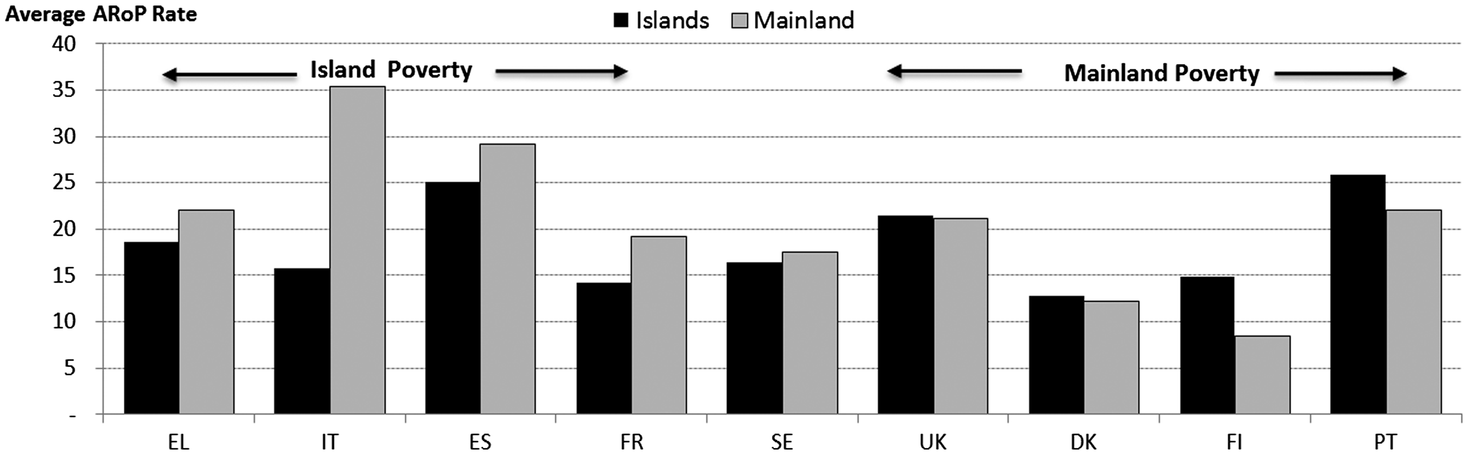
Taken together, the poverty maps, and the graphical analysis based on all the typologies considered by the TiPSE project, suggest the following observations about the geography of income poverty:
At a macro-scale the highest rates of poverty tend to be in the Mediterranean countries and Turkey, the lowest in the Northern and Western countries. The relationship between capital cities, and secondary cities, and ARoP rates is complex. Broadly speaking large cities in the North and West of Europe often contain areas with high rates of income poverty, whilst in the South and East cities tend to have relatively lower rates. Accessible rural areas, especially those close to larger cities and capitals, tend to have relatively low rates of income poverty. Remote rural regions often exhibit relatively high ARoP rates. In some countries island regions have higher ARoP rates than mainland regions. The relationship between mountain regions, border regions and industrial regions and poverty rates is variable, depending upon national and macro-region context.
Associations between poverty rates and some potential socio-economic drivers of poverty
The majority of the ESPON typologies relate to geographical features, rather than socio-economic characteristics. The latter may be explored through correlation analysis with a selection of key indicators from the Eurostat Regio database, and from the Population Census variables collected by the TiPSE project as part of the efforts to map aspects of social exclusion. 11 In choosing indicators the underlying aim is to identify socio-economic characteristics which seem likely to be associated with spatial variations in poverty rates. The selection of indicators will necessarily be constrained by data availability at NUTS 3. It is of course acknowledged that correlations are not evidence of causality, but they may nevertheless provide valuable pointers to policy approaches and targeting.
The selected indicators fall into five broad groups, according to assumptions about the way in which they may be associated with regional variations in the incidence of poverty:
The indicators used in the correlation analysis.

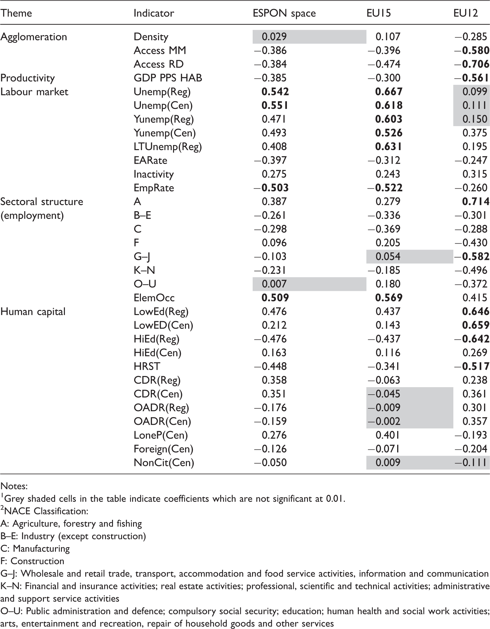
Pearson correlation coefficients between ARoP rates (unadjusted) and selected socio-economic indicators, ESPON space, EU15 and EU12.
Notes:
Grey shaded cells in the table indicate coefficients which are not significant at 0.01.
NACE Classification:
A: Agriculture, forestry and fishing
B–E: Industry (except construction)
C: Manufacturing
F: Construction
G–J: Wholesale and retail trade, transport, accommodation and food service activities, information and communication
K–N: Financial and insurance activities; real estate activities; professional, scientific and technical activities; administrative and support service activities
O–U: Public administration and defence; compulsory social security; education; human health and social work activities; arts, entertainment and recreation, repair of household goods and other services
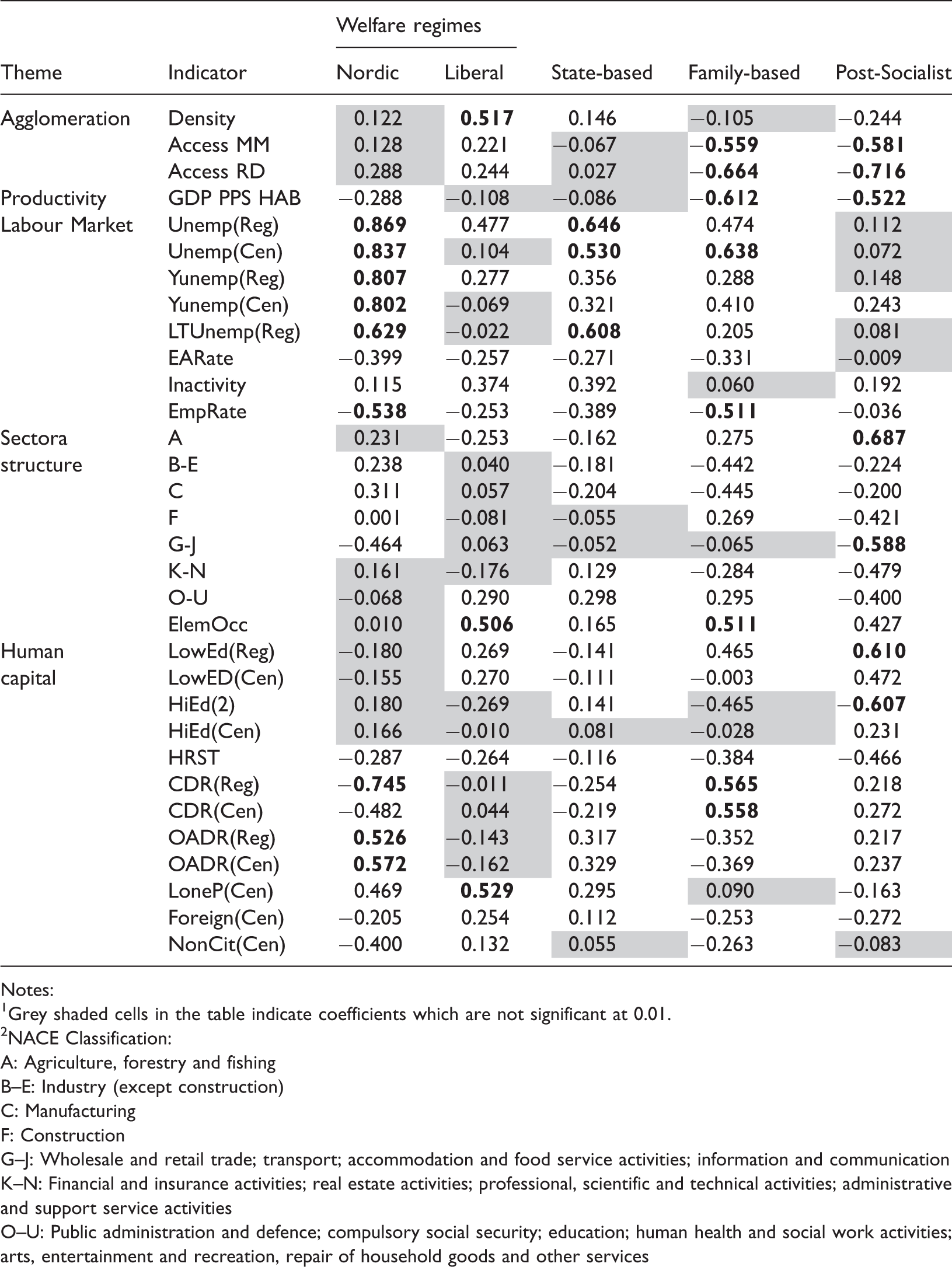
Pearson correlation coefficients between ARoP rates (unadjusted) and selected socio-economic indicators – by welfare regime classification.
Notes:
Grey shaded cells in the table indicate coefficients which are not significant at 0.01.
NACE Classification:
A: Agriculture, forestry and fishing
B–E: Industry (except construction)
C: Manufacturing
F: Construction
G–J: Wholesale and retail trade; transport; accommodation and food service activities; information and communication
K–N: Financial and insurance activities; real estate activities; professional, scientific and technical activities; administrative and support service activities
O–U: Public administration and defence; compulsory social security; education; human health and social work activities; arts, entertainment and recreation, repair of household goods and other services
The ‘ESPON space’ column of Table 3 is based upon the full database of up to 1448 regions. At first sight this may lead us to expect the strongest associations. However, this is not the case, since it is clear from the EU15 and EU12 columns, and from Table 4, that different relationships pertain in different parts of Europe. This perhaps explains the fact that only four indicators have coefficients in excess of ± 0.5. The strongest association, which is sustained across the ESPON space is between poverty rates and unemployment rates (both those derived from the LFS and the Census). Employment rates are also closely related to poverty rates. Youth unemployment rates and long-term unemployment rates are close behind.
Although none of the broad NACE employment sectors have a coefficient above 0.4 (the primary sector reaches + 0.39), employment in elementary occupations shows a relatively strong association with ARoP rates (+0.51). The other three broad groups of indicators, (agglomeration, productivity, and human capital) all have coefficients of less than 0.5, suggesting that if there are relationships with the incidence of poverty they are not consistent across the ESPON space. The closest association from these three broad groups is with educational attainment.
We begin to see different relationships in different parts of the ESPON space as soon as we separate the EU15, from the New Member States (NMS) of the EU12. 12 The difference may be summed up as follows: In the EU15 countries poverty is strongly associated with labour market characteristics and employment in elementary occupations. By contrast, in the NMS accessibility, primary sector employment, education and skills, and productivity are all much more important than labour market characteristics.
The fact that GDP per capita is strongly (negatively) associated with poverty rates in the NMS suggests that here overall performance of regional economies plays a key role, whereas in the EU15 the low correlation coefficient suggests that regional performance is less influential than distributional effects.
The classification of countries according to welfare regime developed in the TiPSE project was based on the work of Esping-Andersen (1994), extended to cover the ESPON area. It is described in more detail in Talbot et al. (2012). This classification suggests some further interesting relationships between ARoP rates and the economic and social characteristics of the constituent regions (Table 4).
Of the five welfare regime groups the strongest and clearest relationship with labour market characteristics is in the Nordic countries, where coefficients rise to > 0.8 for unemployment and youth unemployment. Old age dependency rates are also strongly (positively) correlated with poverty rates in the Nordic states. Child dependency rates have an ambiguous relationship with poverty here, the LFS and Census indicators pointing in opposite directions.
In the liberal welfare regime group (UK and IE) the number of regions is smaller, and it may be that this explains the relatively small number of strong associations. The presence of lone parents, and persons in elementary occupations, is both associated with elevated poverty rates. Population density is also positively associated with poverty, reinforcing the findings presented above, where the UK was one of the few countries in which metropolitan poverty rates were higher than those for non-metropolitan regions.
In the countries with ‘State-based’ welfare regimes, labour market characteristics were again strongly associated with poverty, though youth unemployment was less closely correlated than in the Nordic countries. Here, also unlike the Nordic countries age-related dependency does not seem to play such a strong role. Regional productivity and accessibility/agglomeration are only very weakly associated with poverty here.
Turning to the ‘Family-based’ welfare regimes (the Mediterranean countries and Turkey), accessibility and child dependency rates have distinctive associations with poverty. Overall regional performance (GDP per capita) is also important here. Labour market indicators exhibit less strong associations than in the Nordic countries, 13 whilst employment in elementary occupations is associated as strongly with poverty as it is in the Liberal welfare regime countries.
Finally, the post-socialist countries share certain key characteristics with the previous group, notably the fact that poverty is strongly associated with overall regional economic performance, and with accessibility. However, here education and training, and employment in the primary sector, are also strongly associated with variations in poverty.
Recommendations and suggestions for future research
Given our earlier discussions about the relation between data availability and empirical methodology, we propose the following recommendations:
That (in the short term) NUTS 2 identifiers be included in the EU-SILC microdata for all countries. This would allow increasing the number of countries in which the PovMap methodology could be implemented. That (in the medium term) consideration be given to aligning EU-SILC covariates with the variables of the hyper-tables of the new Eurostat Census Hub. In the longer term, since the trend seems to be increasingly towards register/survey-based systems and away from the conventional census, consideration should be given to specifying regional ARoP rates as an element of the Census Hub hyper-tables. These should be expressed both in terms of national poverty lines and an EU-28 poverty line, adjusted for Purchasing Power Parity. As noted above, poverty measures which take account only of income, whilst ignoring variations in living costs are not always able to identify those most affected by poverty. However to adjust for housing cost but to ignore the very significant cost increases associated with insularity and peripherality would appear to introduce an unintentional urban bias in the indicator. We would therefore recommend that Eurostat and the national statistical institutes explore the possibility of adding standard living cost indicators to the EU-SILC, and using these to adjust regional AROP rates.
Conflict of interest
The author(s) declared no potential conflicts of interest with respect to the research, authorship, and/or publication of this article.
Footnotes
Funding
The author(s) disclosed receipt of the following financial support for the research, authorship, and/or publication of this article:
This publication is based on results of the ESPON project ‘The Territorial Dimension of Poverty and Social Exclusion in Europe (TiPSE)’. © ESPON 2013, TiPSE, Nordregio.