Conducting Three-Level Cross-Sectional Analyses

Abstract

Applied early adolescent researchers often sample students (Level 1) from within classrooms (Level 2) that are nested within schools (Level 3), resulting in data that requires multilevel modeling analysis to avoid Type 1 errors. Although several articles have been published to assist researchers with analyzing sample data nested at two levels, few articles are available to researchers seeking assistance with three-level data analyses. The purpose of this article is to extend the presentational logic and pedagogical flow employed in previous two-level pedagogical publications to illustrate the relevant issues researchers face, the decisions to be made, and the proper procedures needed, when analyzing cross-sectional three-level data. These procedures are demonstrated with a generated three-level data example based on the Early Childhood Longitudinal Study (ECLS-K) public use dataset. The generated data used in this article, as well as the SPSS, SAS, and Mplus model specification syntax files needed to reproduce all analyses in this article, and additional illustrative examples, are available as supplemental online materials at http://jea.sagepub.com/content/early/recent.

Keywords

multilevel modeling three-level modeling cross-sectional HLM SAS SPSS Mplus

Researchers interested in investigating cross-sectional research questions involving early adolescent populations often need to employ clustered sampling designs to obtain an adequate sample size for a given study. For example, a cross-sectional research design might require that early adolescent students (Level 1) be sampled from within several classrooms (Level 2) to obtain adequate statistical power. The need to use multilevel statistical modeling techniques (e.g., hierarchical linear modeling; HLM) to analyze two-level nested data structures that result from such cluster sampling techniques has been well documented (e.g., Raudenbush & Bryk, 2002; Snijders & Bosker, 1999). Researchers interested in the proper procedures needed to analyze cross-sectional data nested at two levels via multilevel modeling can choose from the numerous published pedagogical sources (e.g., Clements, Bolt, Hoyt, & Kratochwill, 2007; Graves & Frohwerk, 2009; Peugh, 2010; Peugh & Enders, 2005; Raudenbush & Bryk, 2002; Singer, 1998; Singer & Willett, 2003; Snijders & Bosker, 1999).

However, adolescent researchers frequently deal with cross-sectional data that is nested at three levels: Students (Level 1) may have been sampled from several classrooms (Level 2) across a number of schools (Level 3). Relative to the pedagogical literature available to guide two-level data analysis efforts, the pedagogical literature available to researchers seeking additional methodological details on cross-sectional three-level analyses is scarce. The goal of this article is to illustrate the steps needed to conduct, present, and interpret the results of cross-sectional three-level analyses using the presentational format, procedural logic, pedagogical flow, and linear model notational schemes (Raudenbush & Bryk, 2002; pp. 228-245) used in the previous two-level modeling pedagogical publications (e.g., Peugh, 2010; Peugh & Enders, 2005; Singer, 1998).

Data Description and Procedural Overview

This article uses simulated three-level cross-sectional sample data modeled after the fifth grade cohort of the ECLS-K (Pollack, Atkins-Burnett, Najarian, & Rock, 2005; Tourangeau, Le, & Nord, 2005; Tourangeau, Nord, Le, Pollack, & Atkins-Burnett, 2006) consisting of (i = 17,565; Level 1) students (coded as STUDENT_ID) nested within (j = 3,158; Level 2) classrooms (coded as CLASSROOM_ID) nested within (k = 992; Level 3) schools (coded as SCHOOL_ID). The three-level cross-sectional example analysis multilevel model used here will examine the effects of student socioeconomic status (SES; Level 1), classroom size (C_SIZE; Level 2), and school tuition cost (TUITION; Level 3) on reading achievement scores (READ_DV) scaled using item response theory (IRT; for a review, see Montague, Penfield, Enders, & Huang, 2010). A model-building procedure will be used to determine the nature and significance of the relationships between student SES, classroom size, and school tuition cost as they affect reading achievement scores.

In general, a model-building approach would first involve including a Level 1 predictor variable such as SES to a multilevel model analysis to determine whether, on average, student SES significantly predicts reading achievement (i.e., a fixed effect). Subsequent model-building steps would involve testing whether the estimated fixed effect of SES on reading achievement shows significant variation across classrooms (i.e., a Level 2 random effect) and across schools (i.e., a Level 3 random effect). A Level 2 predictor of reading achievement, such as classroom enrollment size, could then be entered into the multilevel model to determine whether, on average, classroom size is significantly related to reading achievement; additional model-building steps would determine whether the predictive effect of classroom size on reading achievement varies significantly across schools in a similar fashion.

This model-building approach balances accuracy and parsimony and is prudent for multilevel analyses for three reasons. First, from a pragmatic perspective, researchers are accustomed to specifying the data analytic model dictated by the research question and performing a single analysis (e.g., ANOVA or regression). However, multilevel modeling efforts often do not proceed in such a straightforward fashion. For example, it is well known (e.g., Raudenbush & Bryk, 2002; Singer & Willett, 2003) that model estimation problems (i.e., parameter estimate nonconvergence) tend to increase as the number of random effects increases. As such, it is important to retain only those random effects whose inclusions are critical to properly answering the research question. Second, from a methodological perspective, proper specification of the model under consideration is critical to obtaining accurate parameter estimates. This is especially true for multilevel analyses because the reading achievement score variation that is present across students (Level 1), classrooms (Level 2), and schools (Level 3) is not independent but correlated (shown further below). As such, if a multilevel model is misspecified at Level 1, that misspecification can propagate to higher analysis levels and result in biased parameter estimates at Level 2 and Level 3. Finally, from a functional perspective, proper specification of the multilevel analysis model at all levels (and assuming no estimation errors) enables researchers to clearly interpret fixed effect regression coefficients and random effect variance estimates, as will also be shown below.

The model-building approach described above will be illustrated using SPSS with the ECLS-K simulated dataset to specify and model the effects of student SES, classroom size, and school tuition on reading achievement. The equivalent SAS and Mplus analysis syntax for each of the models shown below is also included in the supplemental online materials (available at http://jea.sagepub.com/content/early/recent). As shown elsewhere (Peugh, 2010; Peugh & Enders, 2005; Singer, 1998), SPSS and SAS use a “combined” multilevel model regression equation (similar to a multiple regression equation) that contains fixed effects for predictor variables, and random effects to address nested data nonindependence, to correctly specify a multilevel analysis model. The combined model is so named because it results from combining the level-specific linear model equations into a large multilevel prediction equation. Only the combined multilevel model equations are given for the multilevel analysis examples presented here. However, the specific Level 1, Level 2, and Level 3 equations¹ for each analysis model illustrated below are shown in the appendix, and detailed descriptions of how the Level 1, Level 2, and Level 3 equations can be merged to form the combined model equations for all the example analyses are included in the supplemental online materials (see “Obtaining the Combined Model” folder at http://jea.sagepub.com/supplemental).

Parameter Estimation and Model Comparison

SPSS and SAS have two options available to researchers for parameter estimation²: full information maximum likelihood (ML) and restricted maximum likelihood (REML). As described elsewhere (e.g., Searle, Casella, & McCulloch, 1992), the two parameter estimation techniques differ only in how fixed effect estimates and their degrees of freedom are treated in estimation. At very large sample sizes (such as the N = 17,565 for the ECLS-K simulated dataset), REML and ML multilevel model parameter estimates are very similar. However, at sample sizes considered typical of applied research, REML gives more accurate estimates of random effects and fixed effect standard errors (Snijders & Bosker, 1999), while ML random effects estimates are negatively biased (Browne & Draper, 2000; Bryk & Raudenbush, 1992; Longford, 1993; Maas & Hox, 2004). REML is used in all multilevel analysis examples shown here because although both estimation methods tend to produce identical fixed effect estimates at large sample sizes, REML gives more accurate random effect estimates at sample sizes more commonly found in research settings.

Further, an important related parameter estimation issue warrants mention. In multiple regression analyses, predictor variables can be tested for significance because, with no cluster sampling and only a single random effect (e_ij), the reference distribution for testing predictors for significance is a t-distribution with known degrees of freedom. In contrast, the appropriate reference distribution for testing predictor variables (fixed effects) in multilevel models is unknown due to cluster sampling and the possibility of unequal sample sizes within Level 2 and Level 3 units, but is typically approximated by a t-distribution with various corrective factors applied to degrees of freedom computations to improve the accuracy of fixed effects significance tests (e.g., see Bauer, Sterba, & Hallfors, 2008). Several degrees of freedom computational corrections are available. Research has shown that the Kenward-Rogers correction (Kenward & Roger, 1997) better maintained the nominal Type 1 error rate for fixed effects significance tests than the Satterthwaite (e.g., Fai & Cornelius, 1996) correction under small sample size, and unbalanced design conditions, especially as multilevel models became more complex and did so without a loss of statistical power (see Schaalje, McBride, & Fellingham, 2002; Spilke, Piepho, & Hu, 2005b). Currently, SPSS (version 20) only offers the Satterthwaite correction for fixed effects tests of significance, but the Kenward-Rogers correction is available in SAS (e.g., Spilke, Piepho, & Hu, 2005a).²

Implicit in a model-building approach to multilevel analyses is the assumption that the parameter estimates added at each stage of the building process significantly improves the fit of the multilevel model to the data. Researchers are often interested in testing whether the parameter estimates added to the multilevel model, whether fixed effects, random effects, or both, result in an improved model fit. Although intuitively appealing to do so, using the single parameter significance tests results of multilevel model analyses can lead researchers to incorrect conclusions regarding model comparisons. Single parameter significance tests, such as the Wald test, for variance estimates (or random effects) assume that the variances are normally distributed in the population when, in reality, they are highly skewed (e.g., Hox, 2010; Pawitan, 2000). As such, Wald tests are contraindicated for model comparison purposes if models differ only in random effect parameter estimates. A likelihood ratio nested model test is needed to compare multilevel models that differ only in one or more random effects (Raudenbush & Bryk, 2002). The steps involved in conducting a likelihood ratio nested model test are reviewed briefly here.

A likelihood ratio nested model test is conducted in three steps. The first step involves estimating two models: a “full” model and a “restricted” model that is nested within the “full” model. Two models are nested if, for example, removing one or more parameters from the “full” model produces the “nested” model. In the second step, the chi-square model fit statistic for the “full” model is subtracted from the chi-square model fit statistic for the “reduced” model (i.e., $Δ χ^{2} = χ_{Reduced}^{2} - χ_{Full}^{2}$ ; or equivalently, [−2LogL_Reduced] − [−2LogL_Full]). In the final step, the chi-square difference statistic ( $Δ χ^{2}$ ; or the −2LogL difference value) computed in the previous step is referred to a chi-square distribution at degrees of freedom equal to the difference in the number of estimated parameters in the “full” and “reduced” model. A significant likelihood ratio nested model test shows that the added parameter estimates in the “full” model significantly improve the fit of the multilevel model to the sample data (see Peugh, 2010 for a more detailed explanation).

Further, if two multilevel models under comparison differ only in two or more predictor variable fixed effect estimates, the likelihood ratio nested model test described above could also be used to conduct a model comparison. However, a more efficient model testing approach is available. Just as an omnibus F-test of an R² statistic tests all the predictor variables included in a multiple regression model as a “set,” a multi-parameter Wald test (e.g., see Hox, 2010, pp. 51-53) tests a “set” of fixed effect estimates added to a multilevel model for a significant improvement in model fit. A multi-parameter Wald test is a more efficient model comparison approach because, rather than estimating a “full” and a “restricted” model, the added predictor variable fixed effects estimates can be tested in the same analysis step by adding the “/TEST” subcommand to the SPSS “MIXED” command (or, with the “/CONTRAST” subcommand for PROC MIXED in SAS), as will be shown below.³

Coding Multilevel Identification Variables in SPSS and SAS

Before presenting the analysis examples, an additional important but rarely mentioned issue regarding the proper nested coding of the identifying (or classifying) variables at all three levels also warrants mention. Researchers often encounter multilevel datasets in which the identifying variables are not explicitly nested. For example, using the ECLS-K simulated dataset as an example, the Level 2 identifying variable (CLASSROOM_ID) might be coded with as many as J = 3,158 different and nonconsecutive values (and by extension, the Level 1 identifying variable [STUDENT_ID] might be coded with as many as I = 17,565 different nonconsecutive values) if the identifying variables were not nested. Nested coding of the identifying variables, for example, involves coding the Level 2 identifying variable (CLASSROOM_ID) with consecutive integer values from 1, 2, . . . to the jth classroom in school k, then restarting the coding of CLASSROOM_ID with consecutive integer values from 1, 2, . . . to the jth classroom within the next k + 1 school, and would continue for all J classrooms within all K schools. The Level 1 identifying variable, STUDENT_ID, could be coded in similar fashion: Students could be coded with consecutive integer values from 1, 2, . . . to the ith student within classroom j, the coding of STUDENT_ID would then restart with consecutive integer values from 1, 2, . . . to the ith student within the next j + 1 classroom, and continue for all I students within all J classrooms within all K schools. This more efficient nested coding scheme, along with the correct Level 2 syntax specification (i.e., RANDOM = | SUBJECT [SCHOOL_ID*CLASSROOM_ID], described below), enables statistical analysis software packages such as SPSS (SAS uses a similar syntax specification) to analyze data nested at three (or more) levels while minimizing the amount of computer memory and computational time needed (e.g., see Kiernan, Tao, & Gibbs, 2012; SAS Institute, 2009). Syntax programs written in SPSS and SAS that recode the identifying variables in the simulated example dataset to a nested format are included in the supplemental online materials⁴ (see “1_Nested Identification Variables” folder at http://jea.sagepub.com/supplemental).

Response Variable Variance and the Intra-Class Correlations

Prior to the estimation of multilevel models that test the effects of predictor variables, estimating an unconditional means three-level model that allows the computation of intra-class correlations (ICC) is considered by many to be a useful initial analysis step (e.g., Peugh, 2010; Peugh & Enders, 2005; Raudenbush & Bryk, 2002; Singer, 1998). The ICC can be defined as the proportion of response variable (i.e., reading achievement) variance present at the student (Level 1), classroom (Level 2), and school (Level 3) levels and also as an estimate of the correlation between the reading achievement scores of two students sampled from the same classroom (Level 2) or the same school (Level 3), as shown below.

The combined linear model for an unconditional three-level analysis is shown in Equation 1 below. Interested readers can find the separate-model (i.e., HLM) equations for all example analyses in the appendix. Interested readers can also find a description in the supplemental online materials (“Obtaining the Combined Model”) of how all the separate-model equations shown in the appendix are integrated to produce all the combined models, such as shown in Equation 1.

Y_{i j k} = γ_{000} + u_{00 k} + r_{0 j k} + e_{i j k} .

In an unconditional means model, the reading achievement score for student i in classroom j within school k (Y_ijk) is modeled as a function of the grand mean reading achievement score for the sample ( $γ_{000}$ ), plus a residual term quantifying school-specific deviations around the grand mean of reading achievement ( $u_{00 k}$ ), plus a second residual term quantifying classroom-specific deviations from the mean of school k ( $r_{0 jk}$ ), plus a third residual term quantifying individual student reading achievement score deviations around the mean of classroom j within school k (e_ijk). As shown in Equation 1, one fixed effect ( $γ_{000}$ ) and three random effects are estimated (Level 3: VAR[ $u_{00 k}$ ] = $τ_{β}$ ; Level 2: VAR[ $r_{0 jk}$ ] = $τ_{π}$ ; and Level 1: VAR[ $e_{ijk}$ ] = $σ^{2}$ ). Using the combined linear model shown in Equation 1 as a guide, the SPSS syntax needed to estimate the 3-level unconditional means model is,

MIXED READ_DV

/PRINT SOLUTION TESTCOV

/METHOD = REML

/FIXED = INTERCEPT

/RANDOM = INTERCEPT | SUBJECT (CLASSROOM_ID*SCHOOL_ID) COVTYPE (ID)

/RANDOM = INTERCEPT | SUBJECT (SCHOOL_ID) COVTYPE (ID).

Prior to linking the combined model shown in Equation 1 to the SPSS syntax above, a brief description of the SPSS MIXED model syntax is needed. For all analyses shown in this article: (a) the reading achievement response variable (READ_DV) is listed immediately after the MIXED command, (b) the /PRINT subcommand controls the output of multilevel analysis results; SOLUTION prints the significance tests for fixed effects (predictor variables), and TESTCOV prints significance tests for random effects (variances), and (c) for reasons described previously, restricted maximum likelihood (/METHOD=REML) estimation was used for all examples shown.

The fixed and random effects shown in the combined model (Equation 1) are specified in SPSS syntax using the FIXED and RANDOM statements. It is important to note that, of the four effects shown in Equation 1 to be estimated, two of the effects are estimated by default. First, the Level 1 random effect ( $σ^{2}$ ) is estimated by default; no syntax specification is needed. Second, the grand mean reading achievement ( $γ_{000}$ fixed effect) is estimated by default unless a no-intercept model is specified by including the “| NOINT” modifier on the /FIXED subcommand line. The remaining two random effects (Level 2 $τ_{π}$ and Level 3 $τ_{β}$ ) are estimated by the two /RANDOM subcommand lines with “| SUBJECT” modifiers. The “/RANDOM = INTERCEPT | SUBJECT (CLASSROOM_ID*SCHOOL_ID)” subcommand line estimates the variation in mean reading achievement scores across classrooms nested within schools (Level 2 $τ_{π}$ ) around the grand mean, while the “/RANDOM = INTERCEPT | SUBJECT (SCHOOL_ID)” estimates the variation in mean reading achievement scores across schools (Level 3 $τ_{β}$ ) around the grand mean. Finally, “COVTYPE(ID)” means that one random effect is estimated at Level 2 and Level 3.

Results for the unconditional means model analysis are shown in the second column of Table 1. The grand mean reading achievement score (i.e., the intercept) was ( $γ_{000}$ = 145.95), and random effect estimates showed statistically significant reading achievement score variation between students (Level 1: σ² = 1,829.49), across classrooms (Level 2: $τ_{π_{000}}$ = 44.75), and across schools (Level 3: $τ_{β_{000}}$ = 446.58). Furthermore, as stated previously, these variance estimates can be used to calculate ICCs that show the proportion of reading achievement variation that exists at all three levels (Raudenbush & Bryk, 2002) as follows:

Table 1.

Model Summaries: Unconditional and Level 1 Examples.

Parameter estimates	Unconditional	SES: Fixed	SES: Random at Level 2	SES: Random at Level 3
Fixed effects
Intercept $γ_{000}$	145.95 (0.77)**	145.91 (0.77)**	145.86 (0.78)**	145.93 (0.77)**
Student SES $γ_{100}$		88.16 (2.83)**	87.62 (3.38)**	87.66 (3.51)**
Random effects
Level 1: Residual $(σ^{2})$	1,829.49 (21.19)**	1,717.17 (19.95)**	1,629.39 (20.07)**	1,634.32 (20.16)**
Level 2: Intercept $(τ_{π_{000}})$	44.75 (13.11)**	64.97 (13.41)**	124.53 (16.88)**	88.42 (14.22)**
Level 2: Covariance $(τ_{π_{010}})$			810.02 (80.39)**	635.83 (80.16)**
Level 2: Slope $(τ_{π_{110}})$			5,268.92 (669.45)**	4,572.53 (886.32)**
Level 3: Intercept $(τ_{β_{000}})$	446.58 (26.73)**	444.92 (26.75)**	438.92 (27.75)**	444.49 (27.05)**
Level 3: Covariance $(τ_{β_{010}})$				214.86 (90.07)*
Level 3: Slope $(τ_{β_{011}})$				990.26 (621.95)†
Model summary
−2 LogL (Deviance)	183,657.48	182,710.91	182,500.37	182,484.29
Number estimated parameters	4	5	7	9

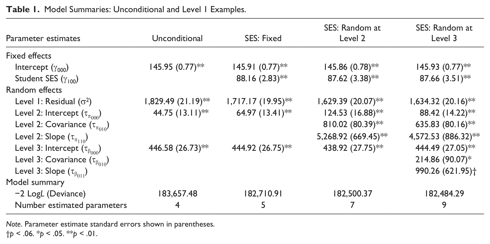
Note. Parameter estimate standard errors shown in parentheses.

†

p < .06. *p < .05. **p < .01.

Level 1 : ICC = σ^{2} / (σ^{2} + τ_{π} + τ_{β}) .

Level 2 : ICC = τ_{π} / (σ^{2} + τ_{π} + τ_{β}) .

Level 3 : ICC = τ_{β} / (σ^{2} + τ_{π} + τ_{β}) .

Substituting the random effect estimates from the second column of Table 1 into Equations 2 to 4 above showed that (1,829.49/[1,829.49 + 44.75 + 446.58] = 0.79) 79% of the reading achievement score variance occurred between students, (44.75/[1,829.49 + 44.75 + 446.58] = 0.02) 2% of the variance occurred across classrooms, and (446.58446.58/ / [1,829.49 + 44.75 + 446.58] = 0.19) 19% occurred across schools. The ICC can also be interpreted as the expected correlation between the reading achievement scores of two students sampled from the classroom (r_Pearson = .02) or the same school (r_Pearson = .19) (see “2_Nested Identification Variables” folder at http://jea.sagepub.com/supplemental).

Level 1 Predictor: Socioeconomic Status

Prior to including one or more Level 1 predictor variables as a first step in the model-building process, researchers need to address the question of how the predictor variables should be centered. Predictor variables in many research disciplines are often measured on an interval scale, meaning that a value of zero has no substantive interpretation (e.g., IQ). In multilevel modeling, this makes interpreting the intercept (i.e., $γ_{000}$ ; the expected reading achievement score when the predictor variable equals zero) difficult. Predictor variable centering is the process of changing the scale of the variable so that a value of zero can be meaningfully interpreted. Although researchers can consult several sources for additional details (Enders & Tofighi, 2007; Hofmann & Gavin, 1998; Peugh, 2010; Raudenbush & Bryk, 2002; Snijders & Bosker, 1999; Wu & Wooldridge, 2005), a brief review of predictor centering is offered here.

Two types of predictor variable centering are available in multilevel modeling: group-mean centering and grand-mean centering. The Level 1 predictor variable student SES will be used in illustrative examples of the two centering options. Group mean centering (also referred to as “centering within cluster”; Enders & Tofighi, 2007) involves subtracting the mean SES value for classroom j in school k $[S E S_{i j k} - {\bar{S E S}}_{j}]$ from the observed SES scores, or subtracting the mean SES value of school k $[S E S_{i j k} - {\bar{S E S}}_{k}]$ from the observed SES scores. Grand-mean centering involves subtracting the sample mean SES value from the SES scores of all students in the dataset $[S E S_{i j k} - \bar{S E S}]$ . A complete discussion of all possible permutations of predictor variable centering, and the interpretational specifics of each, is well beyond the scope of this article. However, a statistical and practical discussion of the two centering options are needed to help clarify an important consideration in multilevel modeling.

As shown previously, the response variable reading achievement showed notable variation and nonzero ICC values at all the three levels. Level 1 predictor variables such as student SES can also show variation and nonzero ICC values at all three levels (i.e., SES_ijk). Statistically, the difference between group-mean and grand-mean centering options is the effect that each has on the ICC values for a Level 1 or a Level 2 predictor variable (e.g., see Enders & Tofighi, 2007). Grand-mean centering has no effect on predictor variable ICC values; a grand-mean centered predictor will still show the same nonzero variation and nonzero ICC values at all levels as it would if it were left un-centered. In contrast, group-mean centering a Level 1 predictor variable such as SES does affect the ICC values. For example, if student SES scores were centered on the mean of their respective classrooms (i.e., $[S E S_{i j k} - {\bar{S E S}}_{j}]$ ), the result is a variable that varies across students (Level 1) but has no variance across classrooms (Level 2) or schools (Level 3) and would have an ICC of zero at Level 2 and at Level 3. Similarly, if student SES scores were centered at the mean of their respective schools (i.e., $[S E S_{i j k} - {\bar{S E S}}_{k}]$ ), the resulting variable would have nonzero variance and nonzero ICC values at Level 1 (students) and Level 2 (classrooms) but zero variance and an ICC = 0 at Level 3 (schools).

From a practical perspective, researchers can be aided in the process of choosing between group-mean and grand-mean centering by considering whether, according to theory, a researcher suspects that the predictor variable will have a relative or absolute effect on the response variable (e.g., see Klein, Dansereau, & Hall, 1994). If the theory under consideration says that a predictor variable would have a relative effect on the response variable—sometimes referred to as a “frog-pond” (Firebaugh, 1980), a “within-groups” (Glick & Roberts, 1984), or a “parts” (Dansereau, Alutto, & Yammarino, 1984) effect—group-mean centering of the predictor variable would be appropriate. One scenario that would indicate the need for group-mean centering would involve two students from families with the same income levels that would be expected to have different reading achievement scores contingent on the classroom they attend (same “frogs” placed in different “ponds”). A second scenario that would indicate the need for group-mean centering would involve a student from a lower SES family that would be expected to have a reading achievement disadvantage if they attend a classroom (within a school) with a higher average income (a smaller income “frog” in a larger income “pond”). Group-mean centering of student SES would be needed in both scenarios because the effect of SES on reading achievement is considered dependent on the kind of classroom (within school) attended. In contrast, if a theory suggested that the impact of SES on reading achievement is independent of the type of classroom (within school) attended, grand-mean centering of student SES is appropriate because a student’s absolute level of SES and its impact on reading achievement, not their SES relative to their classroom peers, are of theoretical interest (for exceptions, see Enders & Tofighi, 2007; Hofmann & Gavin, 1998; Kreft, de Leeuw, & Aiken, 1995). In all analysis examples, student SES was group-mean centered (i.e., student SES scores were centered based on j classroom [Level 2] means $[S E S_{i j k} - {\bar{S E S}}_{j}]$ and this centered variable is referred to as “GROUP_SES” in all SPSS syntax examples below).⁵

The combined linear model that includes group-mean centered SES as a predictor variable is shown below

γ_{000} + γ_{100} (S E S_{i j k} - {\bar{S E S}}_{j}) + u_{00 k} + r_{0 j k} + e_{i j k} .

As shown in Equation 5, two fixed effects (the intercept $[γ_{000}]$ , and the effect of student SES on reading achievement $[γ_{100}],$ ), and three random effects (Level 1: σ², Level 2: $τ_{π_{000}}$ , Level 3: $τ_{β_{000}}$ ) are estimated. The SPSS syntax needed to estimate a Level 1 predictor fixed effect model shown in Equation 5 is,

MIXED READ_DV

/PRINT SOLUTION TESTCOV

/METHOD = REML

/FIXED = INTERCEPT GROUP_SES

/RANDOM = INTERCEPT | SUBJECT (CLASSROOM_ID*SCHOOL_ID) COVTYPE (ID)

/RANDOM = INTERCEPT | SUBJECT (SCHOOL_ID) COVTYPE (ID).

The estimate for the fixed effect of group-mean centered student SES on reading achievement is specified by adding the variable “GROUP_SES” to the “/FIXED =” subcommand line.

Results for the fixed effects Level 1 model are shown in the third column of Table 1. The expected reading achievement score for a student of average SES was ( $γ_{000}$ = 145.91). The incremental effect of SES was ( $γ_{100}$ = 88.16); reading achievement scores increased 88.16 points, on average, for every unit increase in SES. Random effect estimates showed that significant reading achievement variation remained at all three levels (Level 1: σ² = 1,717.17; Level 2: $τ_{π_{000}}$ = 64.97; Level 3: $τ_{β_{000}}$ = 444.92) (see “3_Level-1 Fixed Effect Model” folder at http://jea.sagepub.com/supplemental).

SES Varying Randomly at Level 2

After adding a Level 1 predictor variable such as SES to a multilevel model, a second question for researchers to address is whether the effect of SES on the reading achievement varies significantly across classrooms (Level 2 units). For example, if the effects of student SES on reading achievement were estimated separately for each of the (j = 3,158) classrooms, 3,158 separate $(γ_{1 j k})$ coefficient estimates would result. The mean of the 3,158 coefficient estimates would be $(γ_{100} = 88.16)$ , as shown in Table 1, but the key analysis question is whether the variation in those 3,158 coefficient estimates differs significantly from zero. If so, a term that quantifies classroom-specific variations from the mean effect of student SES on reading achievement would need to be added to the multilevel model to reflect the fact that some classrooms may show more or less than an 88.16 point increase in reading achievement per unit increase in SES.

Specifically, a combined multilevel model that allows the effect of student SES to vary randomly across Level 2 classrooms is defined as

γ_{000} + γ_{100} (S E S_{i j k} - {\bar{S E S}}_{j}) + u_{00 k} + r_{0 j k} + r_{1 j k} (S E S_{i j k} - {\bar{S E S}}_{j}) + e_{i j k} .

The two fixed effects ( $γ_{000}$ and $γ_{100}$ ) and three random effects (Level 1: σ², Level 2: $τ_{π_{000}}$ Level 3: $τ_{β_{000}}$ ) from the previous model are again estimated, along with two additional random effects: the variation in the effect of SES on reading achievement across classrooms (i.e., SES slope variance; $τ_{π_{110}}$ ) and the intercept-slope covariance ( $τ_{π_{010}}$ ; described below). The intercept-slope covariance has been referred to as a “hidden” parameter estimate (Peugh, 2010) because its estimation is not readily apparent from the combined model in Equation 6 or specifically indicated by the syntax example shown below.

The SPSS syntax needed to estimate the effect of SES varying randomly at Level 2 as shown in Equation 6 is,

MIXED READ_DV

/PRINT SOLUTION TESTCOV

/METHOD = REML

/FIXED = INTERCEPT GROUP_SES

/RANDOM = INTERCEPT GROUP_SES | SUBJECT (CLASSROOM_ID*SCHOOL_ID) COVTYPE (UN)

/RANDOM = INTERCEPT | SUBJECT (SCHOOL_ID) COVTYPE (ID).

The addition of “GROUP_SES” to the “/RANDOM | SUBJECT (CLASSROOM_ID*SCHOOL_ID)” subcommand line results in the estimation of the SES slope variance and the intercept-slope covariance by default. “COVTYPE(UN)” specifies an unstructured Level 2 covariance matrix, meaning that SES intercept variance, SES slope variance across classrooms, and the intercept-slope covariance are all estimated as Level 2 random effects.

Results for the model that allows the effect of student SES on reading achievement to vary randomly across classrooms at Level 2 model are shown in the fourth column of Table 1. The expected reading achievement score for a student of average SES ( $γ_{000}$ = 145.86) and the incremental effect of SES ( $γ_{100}$ = 87.62) remained roughly the same as in the previous analysis. Random effect estimates showed that significant reading achievement variation remained at all three levels (Level 1: σ² = 1,629.39; Level 2: $τ_{π_{000}}$ = 124.53; Level 3: $τ_{β_{000}}$ = 438.92). Random effect estimates also showed that the effect of SES on reading achievement varied significantly across classrooms ( $τ_{π_{110}}$ = 5,268.92). Specifically, reading achievement scores could increase by between $(\sqrt{5268.92} = 72.59; 87.62 - 72.59 = 15.03; 87.62 + 72.59 = 160.21)$ 15.03 and 160.21 units for every unit increase in SES. Further, the intercept-slope covariance estimate was also significant $(τ_{π_{010}} = 810.02)$ ; classrooms with more positive SES-reading achievement slopes tend to have higher reading achievement means. The relationship between the resulting SPSS (and SAS) output and the Level 2 covariance matrix $τ_{π}$ is shown below (see “4_Level-1 Effect Random at Level-2” folder at http://jea.sagepub.com/supplemental).

τ_{π} (Level - 2) = [\begin{matrix} U N (1, 1) \\ U N (2, 1) & U N (2, 2) \end{matrix}] = [\begin{matrix} 124.53 \\ 810.02 & 5268.92 \end{matrix}] .

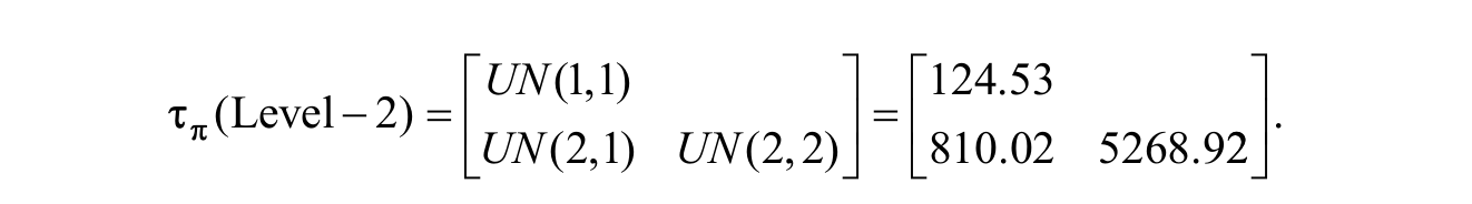
As shown in the third and fourth columns of Table 1, a model that allows the effect of student SES on reading achievement to vary randomly across j classrooms at Level 2 differs from a model that estimates student SES as a fixed effect by only two random effect parameter estimates (i.e., $τ_{π_{010}}$ and $τ_{π_{110}}$ ). As such, the SES fixed effect model is “nested” within a model that allows the effect of student SES on reading achievement to vary randomly across j classrooms (the “full” model) because if the $τ_{π_{010}}$ and $τ_{π_{110}}$ parameters were removed from the SES random effects model (or, if both parameter estimates were fixed at zero), the SES fixed effects model would result. As stated previously, a likelihood ratio nested model test is needed to determine whether the SES random effects model better fits the sample data versus the fixed effects model because the $τ_{π_{010}}$ and $τ_{π_{110}}$ parameters are not normally distributed in the population, and the single-parameter significance tests shown for both in Table 1 are inappropriate for model comparison purposes.

A likelihood ratio nested model test is conducted by first subtracting the relevant model fit statistic for the random effects model (i.e., −2LogL_Full = 182,500.37) from the model fit statistic for the fixed effects model (i.e., −2LogL_Reduced = 182,710.91; Δ-2LogL = 182,710.91 − 182,500.37 = 210.54). In step two, the difference in model fit statistics (Δ-2LogL = 210.54) is referred to a chi-square distribution at degrees of freedom equal to the difference in the number of parameters estimated between the two models under comparison (2, $τ_{π_{010}}$ and $τ_{π_{110}}$ ). The significant likelihood ratio nested model test (i.e., $χ_{2}^{2}$ = 210.54; p < .001) shows that a model that allows the effect of student SES on reading achievement to vary significantly across j classrooms at Level 2 is a significantly better fit to the sample data compared with the SES fixed effect model.

SES Varying Randomly at Level 2 and Level 3

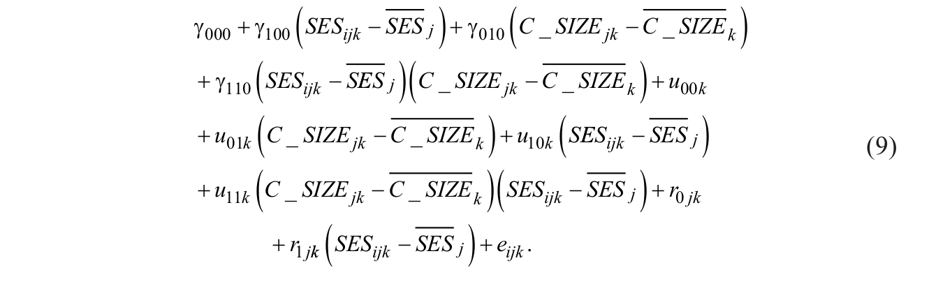
The effect of student SES on reading achievement was shown to vary randomly across (j = 3,158) classrooms. The student SES effect on reading achievement could also vary significantly across (k = 992) schools. A multilevel model that allows the effect of SES on reading achievement to vary across j classrooms and k schools is specified by

\begin{array}{l} γ_{000} + γ_{100} (S E S_{j k} - {\bar{S E S}}_{j}) + u_{00 k} + u_{10 k} (S E S_{j k} - {\bar{S E S}}_{j}) \\ + r_{0 j k} + r_{1 j k} (S E S_{j k} - {\bar{S E S}}_{j}) + e_{i j k} . \end{array}

Two fixed effects are again estimated, the three random effects at Level 2 estimated in the previous model are again estimated, but three additional random effects are now estimated at Level 3 (intercept variance: $τ_{β_{000}}$ , SES slope variance: $τ_{β_{011}}$ , and intercept-slope covariance: $τ_{β_{010}}$ ). The SPSS syntax needed to estimate the effect of SES varying randomly at Level 2 (across classrooms) and Level 3 (across schools), as shown in Equation 7 is,

MIXED READ_DV

/PRINT SOLUTION TESTCOV

/METHOD = REML

/FIXED = INTERCEPT GROUP_SES

/RANDOM = INTERCEPT GROUP_SES | SUBJECT (CLASSROOM_ID*SCHOOL_ID) COVTYPE (UN)

/RANDOM = INTERCEPT GROUP_SES | SUBJECT (SCHOOL_ID) COVTYPE (UN).

Similar to the previous analysis, the addition of “GROUP_SES” to the “/RANDOM | SUBJECT (SCHOOL_ID)” subcommand line results in the estimation of SES slope variance and the intercept-slope covariance (by default) at Level 3, and the “COVTYPE(UN)” statements specify an unstructured covariance matrix at Level 2 and Level 3.

Results for the model allowing the effect of SES on reading achievement to vary randomly at Level 2 and Level 3 are shown in the last column of Table 1. The expected reading achievement score for a student of average SES ( $γ_{000}$ = 145.93) and the incremental effect of SES ( $γ_{100}$ = 87.66) remained relatively unchanged, and all three random effect estimates at Level 2 (intercept: $τ_{π_{000}}$ = 88.42; slope: $τ_{π_{110}}$ = 4572.53, covariance: $τ_{π_{010}}$ = 635.83) remained significant. Random effect estimates at Level 3 showed significant intercept variance ( $τ_{β_{000}}$ = 444.49) and also showed that the effect of SES on reading achievement showed a trend toward significance regarding variation across schools ( $τ_{β_{011}}$ = 990.26). The intercept-slope covariance estimate at Level 3 was also significant ( $τ_{β_{010}}$ = 214.86); schools with larger SES-reading achievement slopes also tend to have higher reading achievement means. The relationship between the Level 2 and Level 3 covariance matrices and the resulting SPSS and SAS output is shown below (see “5_Level-1 Effect Random at Level-2 & Level-3” folder at http://jea.sagepub.com/supplemental):

τ_{π} (Level - 2) = [\begin{matrix} 88.42 \\ 635.83 & 4572.53 \end{matrix}] .

τ_{β} (Level - 3) = [\begin{matrix} 444.49 \\ 214.86 & 990.26 \end{matrix}] .

Level 2 Predictor: Classroom Size

Prior to adding a Level 2 covariate to the multilevel model, it is important to again consider the question of covariate centering. The important question remains whether an absolute or relative effect of the Level 2 covariate classroom size (C_SIZE_jk) on reading achievement is of theoretical interest. Specifically, if a researcher’s theory specified a relative effect of classroom size on reading achievement, such that two classrooms of equal size could have very different classroom mean reading achievement scores based on the different schools to which each classroom belonged, group-mean centering is needed. However, if the absolute effect of classroom size on reading achievement, not the size of a classroom relative to other classrooms in a school is of theoretical interest, grand-mean centering of classroom size is needed. For these examples, classroom size was group-mean centered around each k school’s mean classroom size $(C_S I Z E_{j k} - {\bar{C_S I Z E}}_{k})$ . Further, results of the earlier models showed that the effect of SES on reading achievement varied significantly across classrooms at Level 2. As will be shown below, this raises the possibility that the effect of student SES on reading achievement may be moderated by classroom size (i.e., a cross-level interaction). As shown elsewhere (Enders & Tofighi, 2007; Peugh, 2010), correct covariate centering is essential to the proper interpretation of significant cross-level interaction terms in multilevel models.

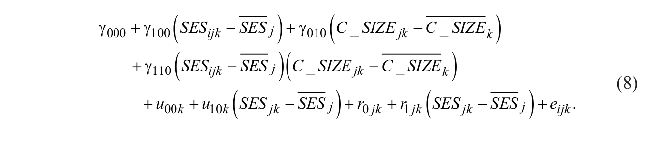
The combined multilevel model that adds the group-mean centered Level 2 predictor variable classroom size $(C_S I Z E_{j k} - {\bar{C_S I Z E}}_{k})$ to the model as a fixed effect is

\begin{array}{l} γ_{000} + γ_{100} (S E S_{i j k} - {\bar{S E S}}_{j}) + γ_{010} (C_S I Z E_{j k} - {\bar{C_S I Z E}}_{k}) \\ + γ_{110} (S E S_{i j k} - {\bar{S E S}}_{j}) (C_S I Z E_{j k} - {\bar{C_S I Z E}}_{k}) \\ + u_{00 k} + u_{10 k} (S E S_{j k} - {\bar{S E S}}_{j}) + r_{0 j k} + r_{1 j k} (S E S_{j k} - {\bar{S E S}}_{j}) + e_{i j k} . \end{array}

Compared with the previous model (Equation 7), two additional fixed effects are estimated. The term $(γ_{010})$ represents the fixed effect estimate of the impact of classroom size on reading achievement, and the term $(γ_{110})$ reflects a cross-level interaction; the effect of student SES on reading achievement moderated by classroom size. As in Equation 7, seven random effects (intercept variance, slope variance, and intercept-slope covariance at Level 2 and Level 3, as well as a Level 1 residual variance) are again estimated.

The SPSS syntax needed to estimate the additional effect of classroom size (shown as GROUP_CLASS_SIZE in all the SPSS syntax examples) on reading achievement as shown in Equation 8 above is,

MIXED READ_DV

/PRINT SOLUTION TESTCOV

/METHOD = REML

/FIXED = INTERCEPT GROUP_SES GROUP_CLASS_SIZE GROUP_CLASS_SIZE*GROUP_SES

/RANDOM = INTERCEPT GROUP_SES | SUBJECT (CLASSROOM_ID*SCHOOL_ID) COVTYPE (UN)

/RANDOM = INTERCEPT GROUP_SES | SUBJECT (SCHOOL_ID) COVTYPE (UN).

/TEST = ALL 0 0 1 1.

The fixed (GROUP_CLASS_SIZE; $γ_{010}$ ) and interaction effects (GROUP_CLASS_SIZE* GROUP_SES; $γ_{110}$ ) involving classroom size are specified by adding both to the “/FIXED” subcommand line. Results for the Level 2 fixed effect covariate model are shown in the second column of Table 2. Neither the fixed effect for classroom size $(γ_{010} = 1.25)$ that quantifies the incremental effect of class size on reading achievement for a student of average SES, nor the (SES*classroom size) interaction effect $(γ_{110} = - 4.58)$ that tests whether classroom size moderates the effect of SES on reading achievement, was statistically significant. All other parameter estimates remained relatively unchanged from the previous analysis. However, it is important to note that if a Level 2 predictor variable is included in the multilevel analysis model, the interpretation of Level 1 predictor variable (SES) parameter estimates changes. For example, $(γ_{100} = 87.69)$ is now defined as the incremental effect of SES on reading achievement for a student attending a classroom at the mean classroom size for a particular k school.

Table 2.

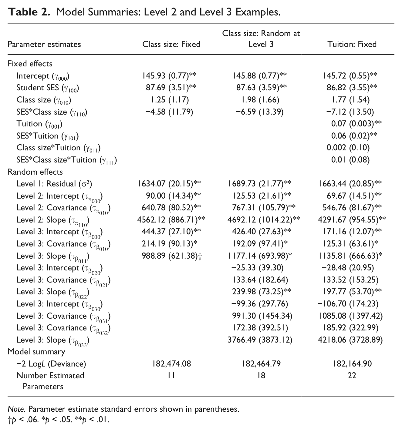
Model Summaries: Level 2 and Level 3 Examples.

Parameter estimates	Class size: Fixed	Class size: Random at Level 3	Tuition: Fixed
Fixed effects
Intercept $(γ_{000})$	145.93 (0.77)**	145.88 (0.77)**	145.72 (0.55)**
Student SES $(γ_{010})$	87.69 (3.51)**	87.63 (3.59)**	86.82 (3.55)**
Class size $(γ_{010})$	1.25 (1.17)	1.98 (1.66)	1.77 (1.54)
SES*Class size $(γ_{110})$	−4.58 (11.79)	−6.59 (13.39)	−7.12 (13.50)
Tuition $(γ_{001})$			0.07 (0.003)**
SES*Tuition $(γ_{101})$			0.06 (0.02)**
Class size*Tuition $(γ_{011})$			0.002 (0.10)
SESClass sizeTuition $(γ_{111})$			0.01 (0.08)
Random effects
Level 1: Residual (σ²)	1634.07 (20.15)**	1689.73 (21.77)**	1663.44 (20.85)**
Level 2: Intercept $(τ_{π_{000}})$	90.00 (14.34)**	125.53 (21.61)**	69.67 (14.51)**
Level 2: Covariance $(τ_{π_{010}})$	640.78 (80.52)**	767.31 (105.79)**	546.76 (81.67)**
Level 2: Slope $(τ_{π_{110}})$	4562.12 (886.71)**	4692.12 (1014.22)**	4291.67 (954.55)**
Level 3: Intercept $(τ_{β_{000}})$	444.37 (27.10)**	426.40 (27.63)**	171.16 (12.07)**
Level 3: Covariance $(τ_{β_{010}})$	214.19 (90.13)*	192.09 (97.41)*	125.31 (63.61)*
Level 3: Slope $(τ_{β_{011}})$	988.89 (621.38)†	1177.14 (693.98)*	1135.81 (666.63)*
Level 3: Intercept $(τ_{β_{020}})$		−25.33 (39.30)	−28.48 (20.95)
Level 3: Covariance $(τ_{β_{021}})$		133.64 (182.64)	133.52 (153.25)
Level 3: Slope $(τ_{β_{022}})$		239.98 (73.25)**	197.77 (53.70)**
Level 3: Intercept $(τ_{β_{030}})$		−99.36 (297.76)	−106.70 (174.23)
Level 3: Covariance $(τ_{β_{031}})$		991.30 (1454.34)	1085.08 (1397.42)
Level 3: Covariance $(τ_{β_{032}})$		172.38 (392.51)	185.92 (322.99)
Level 3: Slope $(τ_{β_{033}})$		3766.49 (3873.12)	4218.06 (3728.89)
Model summary
−2 LogL (Deviance)	182,474.08	182,464.79	182,164.90
Number Estimated Parameters	11	18	22

Note. Parameter estimate standard errors shown in parentheses.

†

p < .06. *p < .05. **p < .01.

Further, as shown in the second column of Table 2, adding the Level 2 predictor variable classroom size as a fixed effect results in a model that differs by two fixed effect parameter estimates only (GROUP_CLASS_SIZE; γ010 and GROUP_CLASS_SIZE* GROUP_SES; γ110) compared with the previous multilevel model that allowed the effect of student SES to vary randomly at Level 2 and Level 3 (see last column of Table 1). As stated previously, a likelihood ratio nested model test could be used to compare the “full” model that adds classroom size as a fixed effect to a “reduced” model that allows the effect of SES to vary across Level 2 and Level 3 units. However, a more efficient multi-parameter Wald test could also be used to compare the two models. As stated previously, multi-parameter Wald tests allow for linear combinations of two or more parameter estimates to be tested for significance as a single “set.” In SPSS, the “/TEST” subcommand is used to request a multi-parameter Wald test. The keyword “ALL” makes all fixed effect and random effect parameter estimates available for additional testing. After the “ALL” keyword, fixed effect contrast coefficients are listed first in the order they appear on the “/FIXED =” subcommand line (if random effects were also to be tested, the “|” symbol would be used to separate fixed effect from random effect contrast coefficients). The first two values of “0” indicate that the intercept $(γ_{000})$ and the SES fixed effect $(γ_{100})$ are not included in the test, while the next two values of “1” specify that the fixed effect for class size $(γ_{010})$ and the SES*class size interaction $(γ_{110})$ , weighted equally, are combined and tested as a “set.” Results of the multi-parameter Wald test (Wald = −3.33; df = 1,578.23; t = −0.28, p = .78) show that including class size $(γ_{010})$ and the SES*class size interaction $(γ_{110})$ did not significantly improve the fit of the multilevel model to the data (SAS [“CONTRAST”] and Mplus [“MODEL TEST:”] examples of the multi-parameter Wald test are included in the supplemental online materials) (see “6_Level-2 Fixed Effect Model” folder at http://jea.sagepub.com/supplemental).

Classroom Size Varying Randomly at Level 3

The results from previous analyses showed that the effect of student SES on reading achievement varied significantly across classrooms and schools. The effect of classroom size on reading achievement could vary significantly across schools in similar fashion. Specifically, although not statistically significant, the main effect of classroom size on reading achievement $(γ_{010} = 1.25),$ and the interaction effect of classroom size by student SES on reading achievement $(γ_{110} = - 4.58)$ could both show significant variation across k schools. The combined multilevel model that allows the effect of classroom size and the classroom size by SES interaction to vary across schools is defined as,

\begin{array}{l} γ_{000} + γ_{100} (S E S_{i j k} - {\bar{S E S}}_{j}) + γ_{010} (C_S I Z E_{j k} - {\bar{C_S I Z E}}_{k}) \\ + γ_{110} (S E S_{i j k} - {\bar{S E S}}_{j}) (C_S I Z E_{j k} - {\bar{C_S I Z E}}_{k}) + u_{00 k} \\ + u_{01 k} (C_S I Z E_{j k} - {\bar{C_S I Z E}}_{k}) + u_{10 k} (S E S_{i j k} - {\bar{S E S}}_{j}) \\ + u_{11 k} (C_S I Z E_{j k} - {\bar{C_S I Z E}}_{k}) (S E S_{i j k} - {\bar{S E S}}_{j}) + r_{0 j k} \\ + r_{1 j k} (S E S_{i j k} - {\bar{S E S}}_{j}) + e_{i j k} . \end{array}

Compared with the previous combined model, two additional random effect estimates ( $u_{01 k}$ and $u_{11 k}$ ) have been added to the Level 3 random effects portion of Equation 9. However, as will be shown below, adding two random effect terms to the combined linear model above results in a notable increase in the number of random effects estimated at Level 3.

The SPSS syntax that allows Level 2 covariate effects to vary randomly at Level 3, as shown in Equation 9 above, is specified as,

MIXED READ_DV

/PRINT SOLUTION TESTCOV

/METHOD = REML

/FIXED = INTERCEPT GROUP_SES GROUP_CLASS_SIZE GROUP_CLASS_SIZE*GROUP_SES

/RANDOM = INTERCEPT GROUP_SES | SUBJECT (CLASSROOM_ID*SCHOOL_ID) COVTYPE (UN)

/RANDOM = INTERCEPT GROUP_SES GROUP_CLASS_SIZE GROUP_CLASS_SIZE*GROUP_SES

|SUBJECT (SCHOOL_ID) COVTYPE (UN).

Allowing the main (GROUP_CLASS_SIZE; $γ_{010}$ ) and interaction effects (GROUP_CLASS_SIZE* GROUP_SES; $γ_{110}$ ) involving classroom size to vary randomly across schools is specified by adding both to the “/RANDOM | SUBJECT(SCHOOL_ID)” subcommand line. Results for the model that allows the Level 2 effects to vary randomly at Level 3 are shown in the third column of Table 2. The four fixed effect estimates remained essentially unchanged from the previous analysis, as did the Level 1 residual variance. Although the intercept variance $(τ_{π_{000}} = 125.53)$ , slope variance $(τ_{π_{110}} = 4692.12)$ , and intercept-slope covariance $(τ_{π_{010}} = 767.31)$ random effect estimates at Level 2 remained significant, the coefficient estimates for each increased as a result of the addition of the Level 3 random effect estimates.

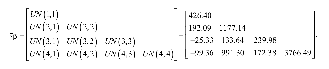
Interpretation of the Level 3 random effect estimates begins by clarifying the relationship between the Level 3 covariance matrix ( $τ_{β}$ ) and the SPSS or SAS output from the analysis that allows the effect of classroom size to vary at Level 3.

τ_{β} = [\begin{matrix} \begin{matrix} U N (1, 1) \\ U N (2, 1) & U N (2, 2) \end{matrix} & \begin{matrix}  \end{matrix} \\ \begin{matrix} U N (3, 1) & U N (3, 2) \\ U N (4, 1) & U N (4, 2) \end{matrix} & \begin{matrix} U N (3, 3) \\ U N (4, 3) & U N (4, 4) \end{matrix} \end{matrix}] = [\begin{matrix} \begin{matrix} 426.40 \\ 192.09 & 1177.14 \end{matrix} & \begin{matrix}  \end{matrix} \\ \begin{matrix} - 25.33 & 133.64 \\ - 99.36 & 991.30 \end{matrix} & \begin{matrix} 239.98 \\ 172.38 & 3766.49 \end{matrix} \end{matrix}] .

As shown in the third column of Table 2 and in the Level 3 random effects covariance matrix ( $τ_{β}$ ), significant variation remained in reading achievement scores across schools $(τ_{β_{000}} = 426.40)$ . Significant variation in the effect of SES on reading achievement also remained $(τ_{β_{011}} = 1177.14)$ . Although classroom size was not significantly related to reading achievement $(γ_{010} = 1.98)$ , Level 3 random effect estimates showed that the effect of classroom size on reading achievement varied significantly across schools $(τ_{β_{022}} = 239.98)$ . However, the student SES by classroom size interaction effect on reading achievement did not vary significantly across schools $(τ_{β_{033}} = 3766.49) .$ . The remaining six random effect estimates shown in the third column of Table 2, and in the covariance matrix ( $τ_{β}$ ), represent all possible pair-wise covariance estimates among the four random effects at Level 3 (see “7_Level-2 Effect Random at Level-3” folder at http://jea.sagepub.com/supplemental).

Level 3 Predictor: School Tuition

Just as in the previous models, the issue of covariate centering should be again addressed before adding an additional predictor variable to the multilevel model. However, grand-mean centering (TUITION_k − $\bar{T U I T I O N}$ ) is the only option for a Level 3 predictor variable such as school tuition because Level 3 variable scores are the same for all students in a school, making group-mean centering impossible. A combined multilevel model that adds the Level 3 covariate school tuition to the multilevel model as a fixed effect covariate is specified by

\begin{array}{l} γ_{000} + γ_{100} (S E S_{i j k} - {\bar{S E S}}_{j}) + γ_{010} (C_S I Z E_{j k} - {\bar{C_S I Z E}}_{k}) \\ + γ_{001} (T U I T I O N_{k} - \bar{T U I T I O N}) + γ_{110} (C_S I Z E_{j k} - {\bar{C_S I Z E}}_{k}) (S E S_{i j k} - {\bar{S E S}}_{j}) \\ + γ_{101} (T U I T I O N_{k} - \bar{T U I T I O N}) (S E S_{i j k} - {\bar{S E S}}_{j}) + γ_{011} (T U I T I O N_{k} - \bar{T U I T I O N}) \\ (C_S I Z E_{j k} - {\bar{C_S I Z E}}_{k}) + γ_{111} (T U I T I O N_{k} - \bar{T U I T I O N}) (C_S I Z E_{j k} - {\bar{C_S I Z E}}_{k}) \\ (S E S_{i j k} - {\bar{S E S}}_{j}) + u_{00 k} + u_{10 k} (S E S_{i j k} - {\bar{S E S}}_{j}) + u_{01 k} (C_S I Z E_{j k} - {\bar{C_S I Z E}}_{k}) \\ + u_{11 k} (C_S I Z E_{j k} - C_{\bar{S I Z E}}_{k}) (S E S_{i j k} - {\bar{S E S}}_{j}) + r_{0 j k} + r_{1 j k} (S E S_{i j k} - {\bar{S E S}}_{j}) + e_{i j k} . \end{array}

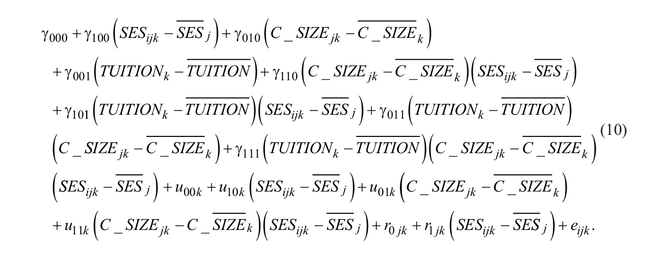
The main effects of SES $(γ_{100})$ , classroom size $(γ_{010})$ , and school tuition $(γ_{001})$ , as well as the student SES by classroom size interaction effect $(γ_{110})$ on reading achievement are all estimated. In addition, the two-way interaction effects of student SES by school tuition $(γ_{101})$ and classroom size by school tuition $(γ_{011})$ , as well as a three-way interaction effect of student SES by classroom size by school tuition $(γ_{111})$ on reading achievement are all estimated. The same random effects are estimated as in the previous model.

The SPSS syntax that adds the grand-mean centered Level 3 predictor variable school tuition cost (shown as GRAND_TUITION in the SPSS and SAS syntax) to the multilevel model, as shown in Equation 10 above, is specified as,

MIXED READ_DV

/PRINT SOLUTION TESTCOV

/METHOD = REML

/FIXED = INTERCEPT GROUP_SES GROUP_CLASS_SIZE GRAND_TUITION

GROUP_SES*GROUP_CLASS_SIZE GROUP_SES*GRAND_TUITION GROUP_CLASS_SIZE*GRAND_TUITION GROUP_SES *GROUP_CLASS_SIZE*GRAND_TUITION

/RANDOM = INTERCEPT GROUP_SES | SUBJECT (CLASSROOM_ID*SCHOOL_ID) COVTYPE (UN)

/RANDOM = INTERCEPT GROUP_SES GROUP_CLASS_SIZE GROUP_CLASS_SIZE*GROUP_SES |SUBJECT (SCHOOL_ID) COVTYPE (UN).

The estimation of the main effect of school tuition (GRAND_TUITION), the two-way interaction effects of student SES by school tuition (GROUP_SES*GRAND_TUITION) and classroom size by school tuition (GROUP_CLASS_SIZE*GRAND_TUITION), and the three-way interaction effect of student SES by classroom size by school tuition (GROUP_SES *GROUP_CLASS_SIZE*GRAND_TUITION) on reading achievement are all specified by adding those four effects to the “/FIXED =” subcommand line.

Results for the Level 3 model are shown in the final column of Table 2. Neither the two way class size by school tuition interaction $(γ_{011} = . 002)$ that tests whether the effect of SES on reading achievement is moderated by school tuition nor the three-way student SES by class size by school tuition interaction $(γ_{111} = . 01)$ that tests whether the effect of SES on reading achievement was moderated by classroom size and school tuition was significant. In addition, the fourteen random effects remained relatively unchanged from the previous analysis with one noteworthy exception. The variation in reading achievement scores across schools $(τ_{β_{000}} = 171.16)$ decreased notably from the previous analysis as a result of adding the four school tuition-related effects to the Level 3 model. Further, the fixed effects estimates for the main effect of school tuition $(γ_{001} = . 07)$ that quantifies the expected increase in reading achievement as school tuition increases for a student of average SES in a classroom of average size, and the student SES by school tuition cross-level interaction $(γ_{101} = . 06)$ that quantifies the extent to which the impact of SES on reading achievement is moderated by school tuition, were significantly related to reading achievement (see “8_Level-3 Effect Model” folder at http://jea.sagepub.com/supplemental). Although not included here in the interests of space, the step-by-step procedure used to graphically display the cross-level interaction of school tuition moderating the effect of student SES on reading achievement (shown in Figure 1) and the steps used to compute multilevel model effect sizes (see Peugh, 2010; Raudenbush & Bryk, 2002; Singer & Willett, 2003) for the final theoretical model of interest have been included in the supplemental online materials (see “Graphically Displaying Cross-Level Interactions” and “Computing Multilevel Effects Sizes” folders at http://jea.sagepub.com/supplemental).

Figure 1.

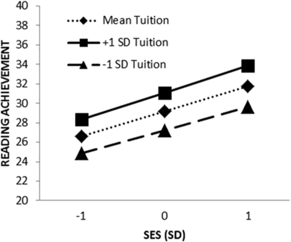
Effect of student SES and school tuition on reading achievement.

A Suggested Ten-Question Multilevel Model Checklist

Researchers face many decisions prior to, during, and following multilevel model analyses in the process of answering research questions that require multilevel analysis techniques. As such, researchers can then be faced with the daunting task of summarizing all the decisions made, techniques used, and results obtained in a manner that can be clearly understood by a target audience. Offered below, in the form of a checklist, are 10 questions that can guide researchers in their multilevel modeling summarization and presentation efforts:

Has the research question been clearly articulated, and a description of the higher level nesting units (e.g., classrooms at Level 2 and schools at Level 3) and all predictor variable(s), control covariate(s), and response variable(s) described?

Has a clear connection been established between the research question and the model-building steps needed to answer the question accurately?

Has the choice of parameter estimation method (ML, REML, MLR) and associated issues (e.g., the chosen denominator degrees of freedom correction method used in SAS) been discussed?

Have the choices and rationales for centering of all continuous and categorical predictor variables been presented?

Have the linear model equations (i.e., the combined model equation [for SPSS and SAS analyses], or the Level 1, Level 2, and Level 3 equations [for Mplus or HLM analyses]) been presented and discussed?

Have all the multilevel parameter estimates (fixed and random effects) been interpreted in the context of the research question?

Have results been summarized in table form (see Tables 1 and 2) in a way that can be linked back to the model equations that allow readers to understand the model tested and the results obtained?

Have the appropriate model comparison tests (likelihood ratio nested model tests or multi-parameter Wald tests) been presented and their implications for a model-building process discussed?

Have any statistically significant interaction effects been presented graphically as well as discussed in text?

Have global (pseudo-R²) and local (PRV) effect sizes been presented for the model(s) of theoretical interest?

Summary and Conclusion

The primary goal of this article was to expand on the previous procedural logic and presentational flow of published articles that have demonstrated the steps needed to analyze two-level nested data to consider the nested three-level cross sectional data analysis case. A secondary goal of this article was to illustrate a model-building process that helps to (a) reduce the possibility of parameter estimation errors and un-interpretable parameter estimates, (b) ensure correct multilevel model specification, and (c) reduce the possibility of parameter estimate bias being propagated throughout the multilevel model. In addition, researchers face numerous important decisions prior to (e.g., choice of parameter estimator and denominator degrees of freedom correction), during (e.g., predictor variable centering and random effect estimation), and following (displaying results tabular and graphical form and computing global and local effect sizes) multilevel modeling analyses. These decisions have been integrated into a suggested checklist to help guide researchers’ efforts in conceptualizing, analyzing, summarizing, and presenting their research findings. Finally, although SPSS syntax was used for all example analyses, (SAS and Mplus syntax for all analysis examples are available in the supplemental online materials), the necessary methodological considerations and needed statistical analysis steps have been presented in sufficient detail to allow researchers to use the multilevel modeling statistical analysis software package of their choice.

Footnotes

Appendix

Acknowledgements

The author wishes to extend his appreciation and gratitude to Tashia Abry, Craig K. Enders, Ting Sa, Yelena Wu, and several anonymous reviewers for their insightful comments and helpful suggestions that greatly improved the quality of this manuscript.

Declaration of Conflicting Interests

The author(s) declared no potential conflicts of interest with respect to the research, authorship, and/or publication of this article.

Funding

The author(s) received no financial support for the research, authorship, and/or publication of this article.

Notes

Author Biography

James L. Peugh is an assistant professor of pediatrics, and has a joint appointment as a quantitative psychologist and a biostatistician at the Cincinnati Children’s Hospital Medical Center. His research focuses on the use of Monte Carlo simulation techniques to test advanced cross-sectional, longitudinal, and multilevel latent variable (continuous and categorical) structural equation models. He has publications in a variety of quantitative, educational, and psychological journals.

References

Bauer

D. J.

Sterba

S. K.

Hallfors

D. D.

(2008). Evaluating group-based interventions when control participants are ungrouped. Multivariate Behavioral Research, 43, 210-236.

Browne

W. J.

Draper

(2000). Implementation and performance issues in the Bayesian and likelihood fitting of multilevel models. Computational Statistics, 15, 391-420.

Bryk

Raudenbush

S. W.

(1992). Hierarchical linear models for social and behavioral research: Applications and data analysis methods. Newbury Park, CA: Sage.

Clements

M. A.

Bolt

Hoyt

Kratochwill

T. R.

(2007). Using multilevel modeling to examine the effects of multitiered interventions. Psychology in the Schools, 44, 503-513.

Dansereau

Alutto

J. A.

Yammarino

F. J.

(1984). Theory testing in organizational behavior: The variant approach. Englewood Cliffs, NJ: Prentice Hall.

Enders

C. K.

Tofighi

(2007). Centering predictor variables in cross-sectional multilevel models: A new look at an old issue. Psychological Methods, 12, 121-138.

Fai

A. H. T.

Cornelius

P. L.

(1996). Approximate F-tests of multiple degree of freedom hypotheses in generalized least squares analyses of unbalanced split-plot experiments. Journal of Statistical Computing and Simulation, 54, 363-378.

Firebaugh

(1980). Groups as contexts and frog ponds. Issues in Aggregation, 43, 52.

Glick

W. H.

Roberts

(1984). Hypothesized interdependence, assumed independence. Academy of Management Review, 9, 722-735.

10.

Graves

Frohwerk

(2009). Multilevel modeling and school psychology: A review and practical example. School Psychology Quarterly, 24, 84-94.

11.

Hofmann

D. A.

Gavin

M. B.

(1998). Centering decisions in hierarchical linear models: Implications for research in organizations. Journal of Management, 24, 623-641.

12.

Hox

J. J.

(2010). Multilevel analysis methods: Techniques and applications. New York, NY: Routledge.

13.

Kenward

M. G.

Roger

J. H.

(1997). Small sample inference for fixed effects from restricted maximum likelihood. Biometrics, 53, 983-997.

14.

Kiernan

Tao

Gibbs

(2012). Tips and strategies for mixed modeling with SAS/STAT procedures (Paper 332-2012). SAS Global Forum, Orlando, Florida. Available at: http://support.sas.com/resources/papers/proceedings12/332-2012.pdf

15.

Klein

K. J.

Dansereau

Hall

R. J.

(1994). Levels issues in theory development, data collection, and analysis. Academy of Management Review, 19, 195-229.

16.

Kreft

I. G. G.

de Leeuw

Aiken

L. S.

(1995). The effect of different forms of centering in hierarchical linear models. Multivariate Behavioral Research, 30, 1-21.

17.

Longford

N. T.

(1993). Random coefficient models. New York, NY: Oxford University Press.

18.

Maas

C. J.

Hox

J. J.

(2004). The influence of violations of assumptions on multilevel parameter estimates and their standard errors. Computational Statistics & Data Analysis, 46, 427-440.

19.

Montague

Penfield

R. D.

Enders

Huang

(2010). Curriculum-based measurement of math problem solving: A methodology and rationale for establishing equivalence of scores. Journal of School Psychology, 48, 39-52.

20.

Muthén

L. K.

Muthén

B. O.

(1998-2012). Mplus user’s guide (7th ed.). Los Angeles, CA: Author.

21.

Pawitan

(2000). A reminder of the fallibility of the Wald statistic: Likelihood explanation. American Statistician, 54, 54-56.

22.

Peugh

J. L.

(2010). A practical guide to multilevel modeling. Journal of School Psychology, 48, 85-112.

23.

Peugh

J. L.

Enders

C. K.

(2005). Using the SPSS mixed procedure to fit cross-sectional and longitudinal multilevel models. Educational and Psychological Measurement, 65, 717-741.

24.

Pollack

J. M.

Atkins-Burnett

Najarian

Rock

D. A.

(2005). Early Childhood Longitudinal Study, Kindergarten Class of 1998–99 (ECLS–K). Psychometric Report for the Fifth Grade. Washington, DC: National Center for Education Statistics, US Department of Education.

25.

Raudenbush

S. W.

Bryk

A. S.

(2002). Hierarchical linear models: Applications and data analysis methods (2nd ed.). Thousand Oaks, CA: Sage.

26.

SAS Institute. (2009). SAS Note 37057 “How large of a hierarchical linear model (HLM) can PROC MIXED fit?” Cary, NC: Author. Retrieved from support.sas.com/kb/37/057.html

27.

Schaalje

G. B.

McBride

J. B.

Fellingham

G. W.

(2002). Adequacy of approximations to distributions of test statistics in complex linear models. Journal of Agricultural, Biological, and Environmental Statistics, 7, 512-524.

28.

Searle

S. R.

Casella

McCulloch

C. E.

(1992). Variance components. New York, NY: Wiley.

29.

Singer

J. D.

(1998). Using SAS PROC MIXED to fit multilevel models, hierarchical models, and individual growth models. Journal of Educational and Behavioral Statistics, 24, 323-355.

30.

Singer

J. D.

Willett

J. B.

(2003). Applied longitudinal data analysis: Modeling change and event occurrence. New York, NY: Oxford University Press.

31.

Snijders

T. A. B.

Bosker

R. J.

(1999). Multilevel analysis: An introduction to basic and advanced multilevel modeling. London, England: Sage.

32.

Spilke

Piepho

H. P.

(2005a). Analysis of unbalanced data by mixed linear models using the mixed procedure of the SAS system. Journal of Agronomy and Crop Science, 191, 47-54.

33.

Spilke

Piepho

H. P.

(2005b). A simulation study on tests of hypotheses and confidence intervals for fixed effects in mixed models for blocked experiments with missing data. Journal of Agricultural, Biological, and Environmental Statistics, 10, 374-389.

34.

Tourangeau

Nord

(2005). Early Childhood Longitudinal Study, Kindergarten Class of 1998-99 (ECLS-K), Fifth-Grade Methodology Report. Washington, DC: National Center for Education Statistics, US Department of Education.

35.

Tourangeau

Nord

Pollack

J. M.

Atkins-Burnett

(2006). Early Childhood Longitudinal Study, Kindergarten Class of 1998-99 (ECLS-K), Combined User’s Manual for the ECLS-K Fifth-Grade Data Files and Electronic Codebooks. Washington, DC: National Center for Education Statistics, US Department of Education.

36.

Y.-W. B.

Wooldridge

P. J.

(2005). The impact of centering first-level predictors on individual and contextual effects in multilevel data analysis. Nursing Research, 54, 212-216.

Supplementary Material

Please find the following supplemental material available below.

For Open Access articles published under a Creative Commons License, all supplemental material carries the same license as the article it is associated with.

For non-Open Access articles published, all supplemental material carries a non-exclusive license, and permission requests for re-use of supplemental material or any part of supplemental material shall be sent directly to the copyright owner as specified in the copyright notice associated with the article.

0.50 MB

1.33 MB

1.31 MB

1.53 MB

1.54 MB

1.58 MB

1.73 MB

0.04 MB

0.06 MB

0.00 MB