Strategic Interaction Among Overlapping Local Jurisdictions

Introduction

Over the last few years, there has been a growing effort to describe the institutional setting of local budgetary decisions. The Fiscal Policy Space (FPS) framework describes five categories of constraints on local fiscal policy: the intergovernmental setting, the economic base, locally imposed fiscal controls, demand for services, and political culture (Pagano & Hoene, 2010). These factors “limit, shape or provide opportunities for policy choices” (p. 248) made by local government officials. This article integrates the FPS framework into Ostrom’s (2007) Institutional Analysis and Development (IAD) framework. This approach is used in this analysis to examine strategic interactions among overlapping local jurisdictions in the context of local fiscal policy.

The type of strategic interaction that may exist between two governments is determined by their geographic and hierarchical position relative to each other. Horizontal interactions occur among neighboring ¹ jurisdictions, while vertical interactions occur among overlapping jurisdictions. These vertical interactions may span across the federal, state, and local tiers of federal government, or alternatively cross overlapping local jurisdictions. School districts, municipalities, counties, and the broad range of special purpose districts exist in a shared local environment.

This study examines how jurisdictional overlap influences property tax rates. Do these local entities mirror each other’s rate setting behavior or do they crowd each other out in competition for the same tax base? Do the strategic interactions occur simultaneously or are they lagged over a multiyear period? Do different types of local governments respond systematically differently to the behavior of their overlapping neighbors? These questions have important fiscal implications for localities. If one type of local government has a strategic advantage in the competition for use of the tax base, then it may crowd out the services provided by the less competitive entity. Alternatively, local governments may take signals from each other about when the time is ripe for increasing general services or issuing debt funded by property tax revenues. Understanding how these interactions influence tax administration is an important aspect of the FPS of local government.

The joining of the FPS and the IAD frameworks allows for an analysis of how the interactions among overlapping jurisdictions create patterns of fiscal behavior. The annual determination of policy is described as an action space that is influenced by environmental constraints. In addition, local government policy actions may create feedback loops that influence those environmental constraints. Berry (2008) identified the property tax base as a common-pool resource shared among local governments and the property owner. The IAD framework is designed to address these specific types of collective action problems.

This article explores the strategic interactions between counties and school districts by testing for reactions to how the property tax is used in overlapping jurisdictions. The analysis uses a rich panel of the financial characteristics of the local governments in the state of Georgia. The data from Georgia are particularly useful because nearly every county in the state has a school district that shares the same boundaries and gross property tax base. Using data on the rates, revenues and bases of each jurisdiction’s property tax as well as information on the other revenues received by each government, this study tests whether property tax levies for both types of governments are established in response to the overlapping jurisdiction’s use of the same base.

The following section provides background on the challenges created by overlapping local governments. The next section presents a theoretical model used to describe strategic interactions. The context of the data collected from local governments in Georga is then described. This is followed by a presentation of the results of the analysis. The paper then ends with a discussion of the implication of the findings for future work on local government finance.

Overview of Local Fiscal Overlap

There is a growing literature investigating the implications of having multiple stacked local jurisdictions providing services and raising revenue within a shared space. Within the public finance literature, the primary concern is to determine how a given jurisdiction’s tax policies are established in response to the policies of their neighbors. A recent series of articles have investigated Local Option Sales Tax rates established by counties and their subsumed municipalities (Burge & Piper, 2012; Burge & Rogers, 2011, 2016). In the first of these articles, Burge and Rogers (2011) estimate the cross-tier tax elasticities between counties and municipalities. The authors find that increases in county local option sales taxes are associated with reductions in municipal property tax bases. Their result is evidence that county-level fiscal decisions have external effects on the cities within their boundaries. This effect creates an incentive for strategic decision making by both levels of government. In a similar vein, Burge and Piper (2012) find that both vertical and horizontal interactions influence counties and municipalities in deciding whether to adopt a local option sales tax. Most recently, Burge and Rogers (2016) investigate the paths of policy diffusion across overlapping jurisdictions. They develop an index to identify leaders and followers in fiscal policy adoption and ultimately are able to measure variation across jurisdictions in their sensitivity to the pressures of tax competition.

Given the importance of the property tax in funding local services, it is notable that relatively little research has been performed on the influence of overlapping jurisdictions on the use of this revenue source. Revelli’s (2001) study of property taxes in the United Kingdom is the only article identified that has examined this issue. His analysis examined the interaction between overlapping districts and county governments in nonmetropolitan regions of England. His analysis found no evidence of any influence from overlapping jurisdictions in the determination of property tax rates.

The implications of overlapping jurisdictions have also been explored in the public budgeting and municipal finance literatures. Goodman (2015) revisits the issues of local government fragmentation’s impact on local spending that were initially raised by Brennan and Buchanan (1980). Goodman finds that the separation of service responsibilities across a greater number of special purpose districts increases the level of aggregate local spending.

Another area of research has focused on the impact of overlapping jurisdictions on the issuance of public debt. Martell (2007) conducts an empirical analysis of Hildreth and Miller’s (2002) conceptual model of how overlapping jurisdictions may influence municipal borrowing costs. Martel’s analysis finds that more fragmented local governments are associated with a reduced debt burden. This surprising result suggests that greater fragmentation among local jurisdictions may reduce borrowing costs. Martel suggests that local governments may closely observe the debt of their overlapping neighbors to avoid becoming subject to a credit downgrade. Greer (2015) builds on Martel’s study by confirming the earlier findings on the relationship between fragmentation and borrowing costs. Greer also examines the impact of an increase on the stock of overlapping debt on a government’s borrowing cost. He finds that increases to the overlapping stock of debt issued by cities, school districts, and special purpose entities increases the True Interest Costs (TIC) of county general obligation debt. This finding is consistent with recommendations in some much earlier accounting literature that overlapping debt should be included in the financial condition assessments of local governments attempting to issue bonds (Petersen, 1977; Raman, 1981).

Another way to frame strategic interaction among overlapping jurisdictions is as a set of institutional constraints. Pagano and Hoene’s (2010) FPS framework was developed as a tool for organizing the various attributes of local government that influence fiscal policy. These are organized into five categories: the intergovernmental context, the economic base, locally imposed fiscal controls, service responsibilities, and the local political culture. Their application of the concept of intergovernmental constraints focused on Tax and Expenditure Limitations (TELs) and intergovernmental service mandates. This article will extend the FPS framework to also include the influence of both vertical and horizontal neighbors’ fiscal policies. The context of this analysis is to assess how a collection of overlapping jurisdictions influence each other’s use of a shared resource—the property tax base. This study will specifically determine the extent that the annual determination of the property tax millage rate is determined strategically with respect to overlapping jurisdictions.

The focus of this study on the institutions that influence the use of a common-pool resource lends itself to being modeled using the IAD framework. The FPS framework offers a way to operationalize the environmental institutions and constraints that are a key part of an IAD model. As shown in Figure 1, the elements of the FPS populate the three clusters of variables that affect the structure of the action arena. In the case of local fiscal policymaking, the action arena is the budgetary process and, specifically for this analysis, the determination of the property tax levy. The three clusters of environmental conditions are the physical and material conditions of the locality, the attributes of the community that the policy is made within, and the rules governing behavior in the community.

OPEN IN VIEWER

Figure 1.

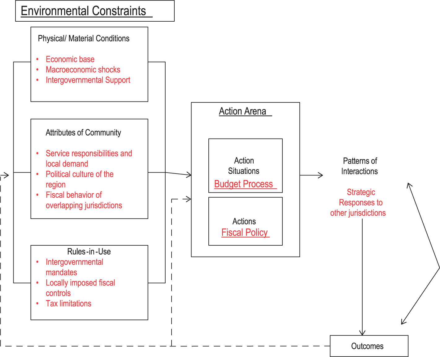
Environmental constraints.

There is an important benefit gained from integrating the concepts of FPS into the IAD framework. The IAD model explicitly recognizes the feedback that flows from action outcomes back into the environmental constraints. This fits the endogenous nature of strategic tax interactions that the public economics literature has modeled for several years (Brueckner, 2003). Recent efforts to apply the FPS framework have framed its institutional constraints as strictly exogenous factors that affect local policy (Hendrick & Crawford, 2014). While this may hold for some of the FPS elements, widening the definition of the intergovernmental setting to include strategic tax determination requires a more dynamic model, and potentially broadens the application of FPS.

The underlying premise of this analysis is that the fiscal policies of a given jurisdiction influence the behavior of the overlapping jurisdictions. Following the notation used by Brueckner (2003), let each jurisdiction i select a level of z i , which in this case is a property tax rate. Government i considers z j in this decision, which is the rate chosen by an overlapping government in the same physical location. The magnitude of z j ’s effect on the choice of z i is the measure of the spillover effect of an overlapping jurisdiction’s policies on local government i. Other attributes of jurisdiction i that affect preferences for public services are described by the vector X i . Officials in jurisdiction i seek to optimize the following objective function:

V ( z i , z j ; X i ) .

Equation 1 is optimized by selecting a level of z i that maximizes V() such that ∂ V / ∂ z i ≡ V z i = 0 . The impact of these factors on the optimal choice of z i is expressed as a reaction function:

z i = R ( z j ; X i ) .

A key feature of a reaction function is that the slope can be either positive or negative. ² A positive sign indicates that local governments follow each other’s fiscal behavior and is consistent with “yardstick” behavior. Observing an increase in z j suggests to jurisdiction i that voters’ demand for public services has increased and it may be an opportune time to increase z i . Alternatively, a negative slope is consistent with a tax competition scenario, where an increase in one jurisdiction’s rate hinders other jurisdictions’ ability to increase revenues. Empirical studies of horizontal interactions among states (Case, Rosen, & Hines, 1993) and local governments (Brueckner & Saavedra, 2001) have estimated positive relationships, finding that geographic neighbors tend to move their tax rates and overall levels in the same direction. Vertical strategic interactions may cause the reaction function to take a negative slope if governments are in competition for use of the same tax base.

Brueckner (2003) notes that applying a reaction function to a vertical interaction is empirically challenging because, “of the inherent asymmetry resulting from consideration of governments at different levels” (p. 182). The relative size of a state to a county or a school district and the differences in the types of taxes they impose and the services they provide make comparison difficult. Within the setting of overlapping local jurisdictions, however, property taxes are imposed on the same gross tax base and the scale of service delivery is much more comparable.

Econometric Model

The development of an empirical framework for estimating Equation 2 begins by transforming it into the following linear form:

z i t = α + γ z i t − 1 + β z j t + θ X i t + ε i t + μ i + τ t .

The i subscript indicates the government unit of analysis, while the j operator indicates the overlapping jurisdiction. The data are measured over t time periods forming a panel data structure. The _i μ i term represents the unobserved characteristics of each jurisdiction that are fixed over time. The τ t term is a set of dummy variables for each time period that capture statewide shocks that would affect property tax policy. The ε i t value represents the error component that is specific to each jurisdiction in a given time period. β measures the effect of a marginal change in an overlapping jurisdiction’s use of the property tax, and θ contains the coefficient estimates for changes in X i t . The equation is additive because all variables have been log-transformed.

The lag of z i t is included in the equation as an explanatory variable. The lagged dependent variable reflects the dependence of the current period’s millage rate on fiscal choices of the previous period. Revelli (2001) interprets this term as the impact of incrementalism in local government tax policy.

Equation 3 is transformed by taking first differences. This transformation eliminates the fixed-effects term, _i μ i , as well as the constant, α . This transformation causes the lagged dependent variable to become correlated with the new error term. The resulting bias in the estimate of γ can be corrected for by instrumenting for Δ z i t − 1 . This is performed using one-step difference Generalized Method of Moments (GMM) regression as described by Arellano and Bond (1991). ³

Given Equation 2, the relationship between ∆z_it Δ z i t and ∆z_jt Δ z j t is endogenous. The β parameter, which measures the impact of jurisdiction j’s policies, is also estimated through the same GMM instrumentation process as Δ z i t − 1 to correct for this endogenity bias. This is performed by using all available lags of the endogenous variables in levels as instruments in first stage equations for each of the endogenous regressors (Roodman, 2007).

To assess the timing of jurisdiction i’s response to ∆z _jt Δ z j t , Δ z j t − 1 is also included in the model. Equation 4 takes the following form:

Δ z i t = γ Δ z i t − 1 + β Δ z j t + κ Δ z j t − 1 + θ Δ X i t + Δ ε i t + τ t .

The sign of β and κ will indicate the type of strategic response to changes in the overlapping jurisdiction’s property tax rate. A positive coefficient estimate is consistent with the “yardstick” model. A negative sign is more consistent with the concept of tax competition and that use of the common tax base reduces overlapping jurisdiction’s ability to generate additional revenue from the same source.

Equation 4 will be estimated for both counties and school districts. The estimates of β and κ will be compared across these two types of local governments to determine whether the strategic response is categorically different. General purpose governments may be more sensitive to the aggregate tax burden because they hold economic development as an explicit policy objective. Special purpose governments like school districts may be more narrowly focused on providing their services and are less concerned with the broader welfare impacts of their tax policies. They may also be more likely to be captured by interest groups focused on maximizing service levels. Goodman’s (2015) finding that increased local government fragmentation is associated with higher per capita expenditures is consistent with capture theory. In the case of school districts, teacher’s unions’ and district officials’ desires to increase educational outcomes may reduce their interest in the fiscal externalities their policies create.

An additional term is added to Equation 4 to capture the influence of geographic neighbors. The average millage rate of neighboring jurisdictions of the same government type is described by ∆z _kt Δ z k t , where k represents the average of all neighboring jurisdictions. Including this term allows the model to control for the influence of both vertical and horizontal strategic interactions. The approach used to identify these neighbors is described in the following section as the method takes advantage of a unique administrative feature of local governments in Georgia. A lag of ∆z _kt Δ z k t Δ z k t is also included in the model. Equation 5 describes the full model.

Δ z i t = γ Δ z i t − 1 + β Δ z j t + κ Δ z j t − 1 + Δ z k t + Δ z k t − 1 + θ Δ X i t + Δ ε i t + τ t .

Data Set

Data Sources

The objective of this analysis is to test whether a county’s choice of property tax levy influences the levy selected by the overlapping school district. Data for this analysis were collected from counties and school districts in the state of Georgia. There are multiple reasons why local governments in Georgia are attractive subjects for investigating the question of overlapping strategic interaction. First, in this state, the fiscal policies of counties and school districts are made autonomously by different sets of local officials. County property tax rates are set by the county Board of Commissioners, while the County Board of Education sets the school district property tax rate. A third entity, the county Board of Tax Assessors is responsible for assessing the value of property for tax purposes. Some states, such as Florida, have mandated state requirements that counties and school districts coordinate the establishment of their property tax rates (Lees, Salvesen, & Shay, 2008). In such a setting, the underlying assumption that county and school district fiscal policy reflects behavior from separate actors is violated. Georgia has no such mandated coordination policy and the overlapping jurisdictions can therefore be viewed as distinct actors.

Second, nearly every county in Georgia also has a countywide school district with which it shares geographic boundaries. For the majority of Georgia counties, ⁴ the school district and the county share the same definition for the gross assessed value of the property tax base. The shared definition of gross tax base means that this analysis is not subject to the problem of asymmetrical tax instruments that challenges most vertical-interaction models (Brueckner, 2003). One caveat, however, is that property taxes levied by school districts and counties are subject to different exemptions provided by state and local governments. The net assessed value for a given property will not be the same for the county tax versus the school tax. I have collected data on the net digest for both types of entities and am therefore able to control for these differences.

A third helpful characteristic of local governments in Georgia is that there are 159 counties in the state. This allows for a large number of vertical interactions to be observed without having to introduce cross-state differences in the legal relationship between local governments. I have collected data on all of the county-school district pairs from 1996 through 2010. Fiscal data were obtained directly from the Georgia Department of Education and from the Georgia Department of Revenue. I also obtained data from the Georgia Department of Community Affairs which collects detailed local government expenditure and revenue data on an annual basis. I also added to this panel data on economic characteristics on the county-level economies collected from the Bureau of Economic Affairs and the Bureau of Labor Statistics. All dollar amounts are also adjusted using the BLS Southern Region Consumer Price Index (1983-1984 = 100).

The primary variable of interest is the property tax rate established by both counties and school districts in Georgia. Figure 2 depicts the average millage rates for both counties and schools along with the average county assessed property value per capita. The rates and the base are depicted together to illustrate that, on average, the property tax rate for both counties and school districts have stayed relatively steady over the 1996 to 2010 period, while real assessed value per capita has grown by about 33%. The bars around each line depict the within-year variation using a 95% confidence interval. Figure 3 depicts the average property tax revenues per capita for counties and school districts over the same period. It shows the same growth trend as the tax base which should be expected given the relative stability of the tax rates over this period.

OPEN IN VIEWER

Figure 2.

Property tax structure of counties and school districts in Georgia 1996-2010 average millage rates and assessed value per capita.

OPEN IN VIEWER

Figure 3.

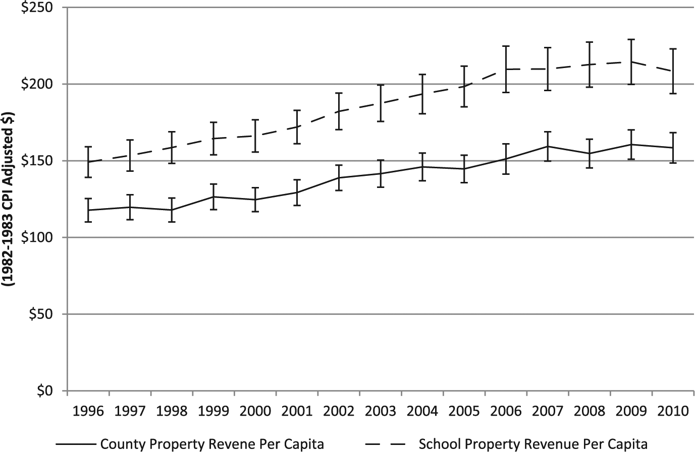
Per capita property tax revenue for Georgia counties and school districts, 1996-2010.

The median home value is not readily available for all counties in Georgia except through the decennial Census Current Population Survey. In nondecennial years, the median home value is only estimated for a subset of Georgia counties. I therefore interpolate the median home value from the average residential parcel value. The Georgia property tax digest separates out each class of property, meaning that it is possible to distinguish residential from agricultural, commercial, and industrial property. Total gross residential assessed property value is divided by the number of residential property parcels in the county to approximate the average residential parcel value. I then calculate the percent change in this value for each county for each year in the panel. I then use this rate of change to interpolate the 2000 Census Current Population Survey (CPS) median home value figure for each county. The ratio of the median home value to the total assessed property value has been used as a measure of the tax price by many models of demand for local government spending since the seminal work by Bergstrom and Goodman (1973).

Two tests were used to measure the accuracy of this method of interpolating the median home value. First, the calculated values were compared with the available Census median home value estimates reported in the American Community Survey (ACS) for 2007-2010. The ACS values were only estimated for 29 counties over those years. T-tests were conducted to determine whether there was a significant difference between the interpolated value and the Census estimates. Running the test separately by year fails to reject the null that the mean difference between the values is 0 for 3 out of the 4 years of data using a .05 alpha level. Using a .01 alpha level fails to reject for each of the 4 years.

As a second test, the annual percent change in the residential parcel value, the basis of the interpolation, was compared with the Federal Housing Finance Agency (FHFA) housing price index. Index values were used from the three Metropolitan Stastical Areas (MSA) located in Georgia: Athens-Clarke County, Atlanta-Sandy Springs, and Augusta-Richmond County. The FHFA price indices were compared with the parcel value growth factor from the counties within those MSAs. ⁵ These figures were compared graphically over the period ranging from 1997 to 2010. This analysis showed a strong similarity in the behavior of the two measures. The results of these two tests allow a degree of confidence in the use of this measure as an approximation of median home value. Dividing this measure of median home value by the net assessed property value for each jurisdiction provides the tax price or the cost to the median homeowner of generating an additional dollar of property tax revenue.

Although both counties and school districts in Georgia are both heavily reliant on the property tax, their dependence on other sources of revenue differs. For counties, the Local Option Sales Tax is the next most important source of revenue, while school districts depend on state aid as the second most important revenue source. County local option sales tax revenue per capita is labeled as SALES, and per capita state aid to school districts is labeled STATE. Both fields are log-transformed.

Income per capita (CAPINC), population density (DEN), and the county employment rate (EMP) are also included in the analysis to control for changes in economic and environmental characteristics that would affect local demand for services. Summary statistics for all variables are presented in Table 1. Note that the home value incorporates Georgia’s 40% assessment ratio, meaning that all property values are assessed for tax purposes at 40% of their actual market value.

OPEN IN VIEWER

Table 1.

Summary Statistics.

	M	SD	Minimum	Maximum
Population	52,670.84	108,203.4	1,698	92,6197
Median home value	22,791.16	10,598.76	6,886.88	69,068.92
Income per capita	13,249.92	2,658.44	7,590.77	31,320.01
School levy per capita	184.75	80.41	46.61	569.96
County levy per capita	128.26	53.8	12.02	453.21
Residential share of gross base	44.15	16.2	5.4	90.86
Employment per capita	0.44	0.13	0.13	1.13
County sales tax per capita	90.11	45.99	1	530.73
State school aid per capita	360.57	84.74	1.83	705.48
County nonsalary benefits per capita	31.91	17.12	1.2	165.83
Percent of county spending on nonsalary benefits	12.29	4.88	0.6	56.34
County general obligation bond debt per capita	37.03	86.74	0	737.95
Farm percent of wages	2.07	5.33	0	62.37
Service sector percent of wages	42.23	14	0	82.73

Although the focus of this analysis is on vertical interaction, it may also be important to control for potential horizontal interactions as well. Integrating both types of competition into a single model would allow for a comparison of the relative magnitude of both effects. The standard approach to measure this is to create a spatial weighting matrix that controls for the attributes of the neighboring jurisdictions. This analysis uses an alternative approach that takes advantage of a feature of the state of Georgia. The counties in Georgia are organized into 12 districts by the Georgia Association of Regional Commissions. The regional commissions are regional planning organizations that engage in a variety of activities that support cooperation among county and municipal governments. These activities include “planning, land-use development, historic preservation, aging services, revolving loan funds, business retention and development, affordable housing, tourism, workforce development, coordinated transportation, geographic information systems, and disaster-mitigation planning” (Walker, 2014). Figure 4 provides a map of the commissions. Membership on the commission includes the chief elected county official, a mayor from within each member county, three residents appointed by the state governor, and two members appointed by the lieutenant governor and the Speaker of the State House of Representatives, respectively (Walker, 2014). These regional governments provide an institutional channel for benchmarking property tax rates among neighboring jurisdictions. The average millage rate for each other ⁶ jurisdiction within a commission for each year is used to measure horizontal neighbors’ tax policies.

OPEN IN VIEWER

Figure 4.

Georgia Association Commissions.

Results

Table 2 presents the results from the analysis using the log of the county millage rate as the dependent variable, while the school district results are in Table 3. Each of the columns in Tables 2 and 3 are organized similarly. Column 1 depicts the one-step difference GMM estimates. One feature of this method is that the number of instruments created through the Arrellano-Bond process is quadratic with respect to the number of time periods. The estimation in column 1 used 199 instruments. Roodman (2007) points out that a high number of instruments, particularly when it exceeds the number of cross-sections, may overfit the endogenous variables and therefore fail to eliminate the bias. In addition, a high number of instruments can weaken the tests for the exogeneity of the instruments and cause them to take unbelievably favorable values. These tests, the Sargan test, the Hansen test, and the difference-in-Hansen tests are reported with their p values at the bottom of each column. The standard practice is to limit the number of instruments to assess the robustness of the results. Column 2 restricts the instruments by only using the first through the third lags of the endogenous variables for GMM-type instruments. This cuts the number of instruments used by a little more than half. Column 3 takes an alternative approach to reducing the number of instruments by “collapsing” the instrument matrix using the procedure outlined by Roodman. Column 4 uses the same collapsed instrumentation strategy used in column 3, but also includes the horizontal tax parameter (∆z _kt) Δ z k t that measures the average millage rate of neighboring jurisdictions within the regional commission.

OPEN IN VIEWER

Table 2.

Dependent Variable: Log of County Millage Rate.

Variables	(1)	(2)	(3)	(4)
	County A-B full	Limited instruments	Collapsed instruments	With horizontal measure
County rate (t − 1)	0.506***	0.575***	0.737***	0.718***
	(0.086)	(0.092)	(0.083)	(0.073)
School rate	0.236	0.404**	1.275***	0.878***
	(0.145)	(0.189)	(0.351)	(0.272)
School rate (t − 1)	–0.198*	–0.283	–0.968***	–0.615***
	(0.120)	(0.182)	(0.268)	(0.214)
Regional average rate				0.488*
				(0.257)
Regional average rate (t − 1)				–0.234
				(0.336)
Tax price	0.061	–0.025	–0.066	–0.048
	(0.045)	(0.047)	(0.046)	(0.044)
ln(income per capita)	0.064	0.098	0.139	0.101
	(0.134)	(0.145)	(0.158)	(0.155)
ln(sales tax rev per capita)	0.018*	0.019*	0.018	0.014
	(0.011)	(0.010)	(0.012)	(0.011)
Pop density	0.062***	0.054***	0.034*	0.028
	(0.022)	(0.020)	(0.017)	(0.018)
Cumulative effect of school rate	0.066	0.285	1.169	0.933
	(0.209)	(0.269)	(0.775)	(0.514)*
Number of id	157	157	157	157
N	1,848	1,848	1,848	1,848
AR1	0.000	0.000	0.000	0.000
AR2	0.617	0.654	0.604	0.680
SARGAN	366.4	223.7	27.99	43.99
SARGAN-P	0	0	0.216	0.117
HANSEN	134.1	76.48	25.31	39.44
HANSEN-p	0.995	0.251	0.334	0.240
difhansen	132	46.15	5.395	17.52
difhansenP	0.960	0.702	0.494	0.419
diff	2.151	30.34	19.92	21.91
diffp	1	0.0240	0.278	0.188
No. of Inst	199	89	43	56

Note. Estimates obtained using One-Step Difference Generalized Method of Moments (GMM) Regression. All variables are first differences.

All tax rates and the tax prices are log-transformed. Dependent variable is the log of the county property tax rate. Robust standard errors in parentheses (clustered by county). Year dummies are included in all models. AR1 and AR2 indicate Autogression tests of the first and second order, respectively.

*

p < .1. **p < .05. ***p < .01.

OPEN IN VIEWER

Table 3.

Dependent Variable: Log of School District Millage Rate.

Variables	(1)	(2)	(3)	(4)
	County A-B full	Limited instruments	Collapsed instruments	With horizontal measure
School rate (t − 1)	0.728*** (0.037)	0.714*** (0.045)	0.763*** (0.058)	0.731*** (0.053)
County rate	0.041 (0.033)	0.070 (0.048)	0.237** (0.108)	0.192** (0.092)
County rate (t − 1)	–0.047* (0.028)	–0.074* (0.042)	–0.204** (0.081)	–0.165** (0.071)
Regional school average rate				–0.073 (0.181)
Regional school average rate (t − 1)				0.104 (0.211)
Tax price	0.010 (0.033)	0.024 (0.031)	0.031 (0.029)	0.026 (0.029)
ln(income per capita)	–0.091 (0.077)	–0.104 (0.087)	–0.108 (0.090)	–0.099 (0.091)
ln(state aid to school districts per capita)	–0.002 (0.004)	–0.003 (0.004)	0.002 (0.004)	0.001 (0.004)
Pop density	–0.007 (0.006)	–0.006 (0.006)	–0.003 (0.008)	–0.004 (0.007)
Cumulative effect of the county rate	–0.023 (0.083)	–0.015 (0.093)	0.137 (0.198)	0.101 (0.149)
Number of id	157	157	157	157
N	1,848	1,848	1,848	1,848
AR1	0	0	0	0
AR2	0.188	0.166	0.224	0.195
SARGAN	175.7	116.9	20.05	35
SARGAN-P	0.555	0.000	0.639	0.420
HANSEN	134.5	76.72	28.35	45.56
HANSEN-p	0.995	0.245	0.203	0.0890
difhansen	143.2	57.61	4.354	21.54
difhansenP	0.853	0.275	0.629	0.203
diff	–8.706	19.11	24	24.02
diffp	1	0.322	0.120	0.119
No. of Inst	199	89	43	56

Note. All variables are first differences. All tax rates and the tax price are log-transformed. Dependent variable is the log of the school property tax rate. Robust standard errors in parentheses (clustered by county). Year dummies are included in all models. AR1 and AR2 indicate Autogression tests of the first and second order, respectively.*p < .1. **p < .05. ***p < .01.

The results presented in Tables 2 and 3 depict how local governments’ determination of their property tax rate is influenced by the choices of overlapping jurisdictions that are also taxing the same property base. This impact can be expressed either as a long-run cumulative effect or as a short-run impact at a given point in time. The individual coefficient estimates must undergo transformations to compute either the long- or short-run effects. Using the notation from Equation 4, the long-run change ⁷ in ∆z_it Δ z i t with respect to a change in ∆z _jt Δ z j t is ( β + κ ) / ( 1 − γ ) . These cumulative effects are presented in Tables 2 and 3 below the individual coefficient estimates. ⁸

Looking first at the aggregate long-run impact of the school rate on the county taxes, the estimates in the four columns of Table 2 indicate that there is almost no lasting effect created by vertical tax competition. The aggregate effects can be interpreted as a long-run elasticity for county rate with respect to changes in the school rate. The first three columns consistently show that the cumulative effect is not significantly significant. Column 4, which adds the horizontal tax competition parameter to the model does reveal a positive and significant effect that is marginally significant. With a point estimate of 0.933, the cumulative impact of changes to the school’s levy on the county levy is approximately unitary elastic. This mixed set of results suggests that the cumulative effect of school district tax policy on county tax rates is either close to zero or a positive effect. There is no indication of a negative effect that would be consistent with the common-pool resource problem predicted by Berry (2008). Instead, the evidence suggest that there is either no long-run impact of school tax increases on county taxes, or there is a positive effect in which increases to the school rate signal to the county to also increase their tax rates.

Table 3 shows that the estimates using the school district rates as the dependent variable. In all four models, the school rates exhibit no cumulative response to changes in the county tax rate. The point estimates of the aggregate effect range between −0.023 and 0.137 and none come close to statistical significance.

Although neither the counties nor the schools show a lasting aggregate effect from the fiscal policies of their overlapping counterparts, the short-run effects do show that both types of government make a temporary response to the tax policies of the overlapping jurisdiction. Using the column 3 results from Table 2, the coefficient on the School Rate variable is estimated to be 1.275. This can be interpreted as the short-run impact of the school rate on the county rate at time t. This suggests that there is a strong simultaneous mimicking effect exhibited by the county governments to changes in the school district rate. One period later, the impact of that initial change in the school rate is expressed in the notation of Equation 4 as ( κ + γ β ). From the estimates of column 3, this calculates as (−0.968 + [0.737 × 1.275]) = −0.028. The following period the size of the effect shrinks dramatically and reverses its sign.

The short-run responses between the overlapping districts can be depicted visually. Figure 5 plots the short-run effects given a change in the overlapping jurisdiction’s rate using the column 3 estimates. The horizontal axis represents the time periods following a percentage change in ∆z _jt Δ z j t . The height of each line is the percent change made in ∆z_it in response in year t. The height of the line at the y axis is the simultaneous response, while the height at year 1 along the x axis is the secondary response in the following year. The cumulative effect reported in Tables 2 and 3 is the sum of the height of the line for all time periods. This graphic reveals that for both counties and school districts there is a strong simultaneous effect so that when one jurisdiction raises its rate the overlapping jurisdiction responds by also raising its rate. One period after the change is made, however, the response is reversed. Sensitivity testing was conducted with multiple additional lags and the results were unchanged.

OPEN IN VIEWER

Figure 5.

Short-run responses to changes in overlapping jurisdiction’s property tax rate.

The key difference between counties and the school districts is that the schools appear to be much less sensitive to the fiscal policies of the counties than the counties are to the school districts. This finding makes practical sense as the schools are special purpose governments that are primarily focused on providing educational services. The county general purpose government would be expected to take a broader view of the economic condition of their jurisdiction as economic development and regional planning are functions of county government in Georgia. The distinction between general and special purpose governments affects the short-run sensitivity to overlapping jurisdictions’ fiscal policies.

One caveat to the short-run difference between counties and schools is that their relative millage rates could explain up to half of the effect. School district millage rates average about 45% higher than the county rates. Since the coefficient estimates are structured as elasticities, the county percent changes would be larger than the school percent changes. As a robustness check, the models were reestimated using the raw millage rates instead of the logged millage rates. This change did reduce the size of the coefficients by about 40%, as expected. The direction and the size of the short-run responses were unchanged. Using the raw millage rates did, however, increase the statistical significance of the positive long-run responses by counties to changes in the schools tax rates. The long-run school responses to the counties were unaffected, having no long-run effect.

Taken together, the aggregate and short-term effects suggest that the strategic interaction between counties and school districts is primarily an immediate mimicking effect that is largely reversed in the subsequent period. The effect of the school rate changes on the county rates may have a persistent upward effect, but it is not a strong relationship.

The impact of the neighboring jurisdictions within the regional commissions also had a minimal effect on the dependent variables. Column 4 of Table 2 shows an elasticity of 0.488 between the neighboring county rates and ∆z_it Δ z i t , though the estimate was only marginally significant. In comparison, the effect of the school districts on the counties was nearly twice as large and the statistical significance of the estimate was an order of magnitude higher. The school districts were even less influenced by the neighboring school districts within the commission areas than the counties were by their neighbors.

None of the other control variables had a consistent statistically significant impact across the specifications.

Discussion

This article presented an empirical analysis of the influence overlapping local jurisdictions have on each other’s tax policies. The analysis focused on answering three questions. The first goal was to determine whether there was any interaction effect and, if there was any, what direction it takes. This analysis produced mixed results as to the size and significance of any long-run cumulative effect. The evidence suggests that there is minimal persistent impact from overlapping jurisdictions, and if there is any effect, it appears to be positive. This result rejects the notion of a strong tax competition effect where one jurisdiction increasing its rate would cause reductions in the overlapping jurisdictions’ rates. This finding of minimal long-run impact is consistent with Revelli’s (2001) analysis of vertical property tax competition in the United Kingdom. The primary dynamic appears to be a temporary mimicking effect that is largely reversed one period after the property tax rate is changed.

This analysis also addresses the secondary goal of determining how the strategic response plays out over time. The short-run interaction between counties and school districts in Georgia appears to occur almost entirely within the year following the rate change. Additional testing was conducted with deeper lags with no change to the results. This analysis builds on Revelli’s (2001) excellent analysis of property tax rates in the United Kingdom by differentiating between the short-run and cumulative effects of overlapping jurisdictions.

The third contribution of this study is to highlight the differential responses made by counties and school districts. Even though the direction of the effect was the same for both types of local government, the schools appeared to be much less sensitive to overlapping competition than the counties did. This finding fits with Berry’s (2008) common-pool framework for vertical interaction in which special function governments are primarily concerned with providing services which benefit their interest group constituency. The school’s focus is on providing educational services and are less concerned with the fiscal policies of the counties on the overall tax base. In addition, because the effect of the interaction for both counties and school districts is temporary, there does not appear to be a significant welfare problem created by strategic interaction between overlapping jurisdictions. A statistically significant aggregate effect in either direction would have suggested that tax competition drives taxes and the corresponding level of public services above or below its equilibrium level. Instead, the observed data suggest that after an initial adjustment both types of jurisdictions return to their original state.

This analysis points toward several additional research questions. First, this analysis focused on the property tax used to finance operating expenditures. The use of property taxes to finance debt may not follow the same pattern of behavior as the decision to issue debt is more visible and may generate greater political costs. Second, the finding that the counties and the school districts exhibited different degrees of sensitivity to their overlapping neighbor’s tax policy begs the question as to how the other types of local jurisdictions respond. Developing an understanding of how other types of special purpose governments respond to the local fiscal environment remains an important research goal.

One next step would be to integrate municipalities into this research. Doing so would significantly complicate the research design, however, because it would lose the perfect boundary overlap between school districts and counties that aided this analysis. Developing a framework to address the asymmetrical relationships between a broader mix of overlapping local jurisdictions will significantly deepen our understanding of the local fiscal environment.

This analysis also demonstrated a broader context for the FPS framework as an application of Ostrom’s IAD Framework to local government budgetary decisions. Using this lens to study the impact of institutional forces on fiscal administration may be a useful approach for future research. Framing the annual budgetary process as an “action space” within the IAD framework and then examining the patterns of fiscal behavior that arise in response to the institutional setting may be a helpful tool for understanding the administrative challenges that emerge in an environment of overlapping jurisdictions.