Proxy pattern-mixture models (PPMMs) have previously been proposed as a model-based framework for assessing the potential for nonignorable nonresponse in sample surveys and nonignorable selection in nonprobability samples. One defining feature of the PPMM is the single sensitivity parameter, , that ranges from 0 to 1 and governs the degree of departure from ignorability. While this sensitivity parameter is attractive in its simplicity, it may also be of interest to describe departures from ignorability in terms of how the odds of response (or selection) depend on the outcome being measured. In this paper, we re-express the PPMM as a selection model in order to better understand the underlying assumptions of the PPMM and the implied effect of the outcome on nonresponse (or selection). The selection model that corresponds to the PPMM is a quadratic function of the survey outcome and proxy variable, and the magnitude of the effect depends on the value of the sensitivity parameter, (missingness/selection mechanism), the differences in the proxy means and standard deviations for the respondent and nonrespondent populations, and the strength of the proxy as measured by the correlation between the outcome and the proxy in the respondent/selected sample. Large values of (beyond ) may result in unrealistic selection mechanisms, and the corresponding selection model can be used to establish more realistic bounds on . We illustrate the results using a home pricing dataset extracted from the China Family Panel Studies.
The proxy pattern mixture model (PPMM) is a method for assessing potentially nonignorable nonresponse bias for the mean of a survey variable subject to nonresponse, when there is a set of covariates observed for nonrespondents and respondents (Andridge and Little 2011). It is a model-based method to create adjusted estimators for situations where nonresponse could be nonignorable and uses a sensitivity analysis to assess how much inference is affected by nonignorable nonresponse. The PPMM provides a simple framework for addressing issues arising from missing data due to nonresponse or issues of selection bias. In the context of missing data, Andridge and Little (2011, 2020) proposed the PPMM as a measure of the potential impact of nonresponse on survey estimates for both continuous and binary outcome variables. Little et al. (2020) used the PPMM as the basis of indices that measure the degree of potential sampling bias arising from the use of nonprobability samples. Andridge et al. (2019) extended this approach to indices of potential nonignorable selection bias for estimates of population proportions. The PPMM and indices derived from the PPMM have subsequently been shown to effectively capture nonignorable nonresponse and/or selection bias in different applications, including state-level pre-election polls in the U.S. and Great Britain (Jackson 2023; West and Andridge 2023), for a variety of outcome measures from the German General Social Survey (Hammon and Zinn 2024), and for estimates of COVID-19 vaccine from large-scale internet-based surveys in the U.S. (Andridge 2024).
The PPMM, unlike other weighting and imputation methods for adjusting for survey nonresponse, does not assume the data are missing at random (MAR) (Andridge and Little 2011, 2020). Rather, it utilizes a single sensitivity parameter () ranging between 0 and 1 that controls the deviation from MAR, where corresponds to MAR and corresponds to missingness depending only on the outcome of interest that is subject to missingness. Little et al. (2020) recommended the use of a central value of , if a single point estimate is desired. The key question is, how “realistic” is a value of (or other values)? The goal of this paper is to connect the PPMM to a selection model framework to help judge the magnitude of nonignorable missingness or selection. Selection models are an alternative modeling method that model the effect of survey outcome, on missingness or selection, and can thus often be more easily interpreted. In Section 2, we briefly review the general framework of the PPMM, and in Section 3 we express the PPMM as a selection model and explore its properties. Section 4 applies the method to a home pricing dataset extracted from the China Family Panel Studies, and Section 5 presents discussion, including extensions of the proposed method.
2. Background: The Proxy Pattern-Mixture Model
Andridge and Little (2011) first introduced the PPMM for assessing the potential for nonresponse bias for continuous outcomes in surveys. Since then, there have been several extensions of the methods to incorporate binary and skewed survey outcome cases (Andridge and Little 2020; Andridge and Thompson 2015a, 2015b; Andridge et al. 2019) and to increase robustness (Yang and Little 2021). The model has also been applied (with some refinements) to the closely related problem of selection bias (Andridge et al. 2019; Boonstra et al. 2021; Little et al. 2020; West et al. 2021), and recently was extended for use in assessing the generalizability of randomized trial results (Andridge et al. 2025). This section contains a brief overview of the PPMM in the context of estimating means; we refer interested readers to the aforementioned references for more details.
2.1. PPMM General Framework for Continuous Survey Outcome
We consider a sample size of units drawn randomly from an infinite population. For the unit in the sample, let denote the value of the continuous survey outcome variable and denote the observed values of covariates. We do not observe the responses of all the subjects in the sample, rather, we only observe the responses of out of the sampled units. Thus, the observed data consists of for and for . Assessing and correcting for the nonresponse bias in the survey outcome mean is of primary interest.
Let denote the response indicator, where when is missing and when is observed. As described by Andridge and Little (2011), we reduce the covariates to a single proxy variable that is a linear combination of the covariates by regressing on using the data for the respondent group, that is, . The proxy variable, , is obtained as the predicted values of the survey outcome from the regression model, and is available for both non-respondents and respondents. Therefore, the proxy is constructed using estimated regression parameters from the observed data, rather than being known exactly. A Bayesian approach can also be used to account for the uncertainty in these proxy values by estimating the proxy and outcome model parameters together, see Andridge and Little (2011) and Little et al. (2020) for details. We note that, as part of this data reduction technique, only variables that are associated with in the respondent sample will contribute to the proxy, as any covariate that is not associated with will have a zero or near-zero coefficient in this regression model. Thus, covariates that are associated with nonresponse but not with the specific variable being studied are not informative for the PPMM analysis. If a large number of variables are available, formal variable selection techniques may be necessary to reduce the number of predictors in the model that creates the proxy. Conceptually, the role of the covariates this framework is to provide information that is associated with the outcome, so that the proxy captures meaningful variation in . In practice, this suggests prioritizing variables that are plausibly related to the outcome, without worrying about interpretation of individual covariate effects.
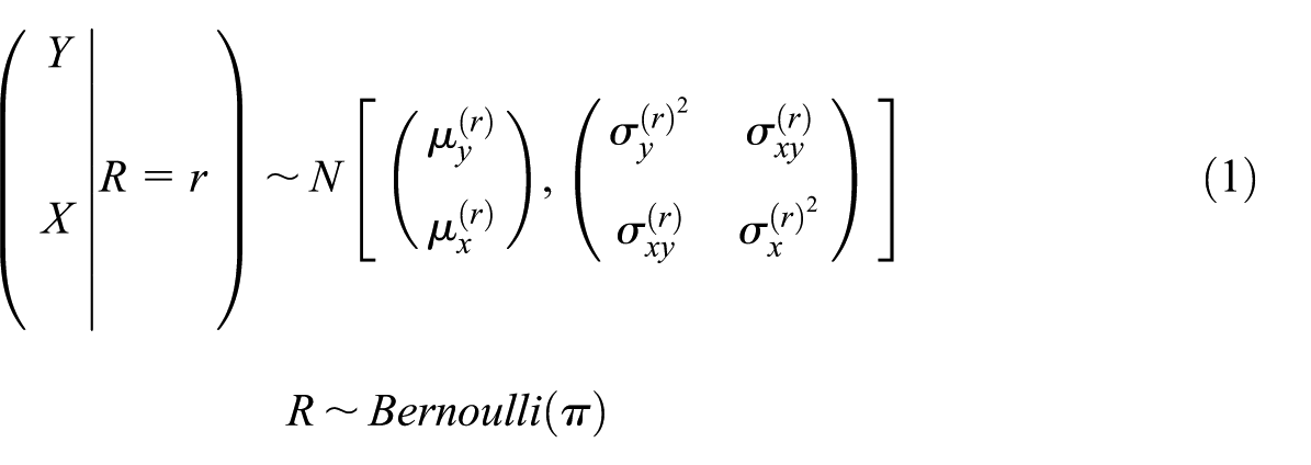
The assumed model for the joint distribution of is:
where is the response rate for the outcome (i.e., ). The parameters , and for non-respondents are unidentifiable without any further assumptions. To identify these parameters from the model, an identifying restriction is imposed on the parameters (Andridge and Little 2011, 2020; Little et al. 2020):
Here, is an unspecified function, is a rescaled (for mathematical convenience) version of the proxy , and is a set of other covariates that are independent of and for units in the respondent sample but that may be related to response (i.e., related to ). The parameter is a sensitivity parameter—there is no information in the data that can be used to estimate it—that is varied to account for a range of assumptions on the missingness mechanism. The relative amount of missingness due to and to is described by the chosen value of , which ranges from to . If , it means that the missingness solely depends on , not , that is, the data are missing at random (MAR). On the extreme side, if , then missingness solely depends on , not , that is, the data are “extremely” missing not at random (MNAR). Values of between 0 and 1 correspond to nonignorable missingness mechanisms where missingness depends in part on the outcome .
Here is the correlation between the outcome and proxy in the respondent sample and is referred to as the “strength” of the proxy. The overall mean for is then the weighted average of the respondent and nonrespondent means, that is, . By either fixing at a single value or putting a prior on (e.g., Uniform(0,1)), one can estimate the mean of under the PPMM and estimate the amount of bias in the respondent mean.
We note that the PPMM as described above assumes that the units were selected via a simple random sample from the target population, such that the unweighted mean is an unbiased estimate of the true population mean. If a complex sampling design was used, the PPMM can still be used to estimate the respondent and nonrespondent means as described above, but additional steps are needed to obtain population-level estimates. Andridge and Little (2011, 2020) describe a multiple imputation (MI) approach, where the PPMM is used to impute the missing outcome values, and then complex design features like clustering, stratification and unequal sampling probabilities can be incorporated in the complete-data component of the MI combining rules.
3. The PPMM as a Selection Model
Pattern-mixture models and selection models are two alternative approaches when dealing with incomplete data and nonignorable missing-data mechanisms (Glynn et al. 2013). Both approaches rely on assumptions that cannot be empirically verified and require additional constraints to fully identify the model. These two approaches make different distributional assumptions, though previous work has shown that these two approaches can sometimes be expressed in equivalent forms when outcomes are in the exponential family (Kaciroti and Raghunathan 2014). In our setting, the PPMM assumes a bivariate normal distribution for the joint distribution of conditional on the response indicator . By restricting the two joint distributions when and to be normal, the implied response mechanism naturally takes the form of a logistic function:
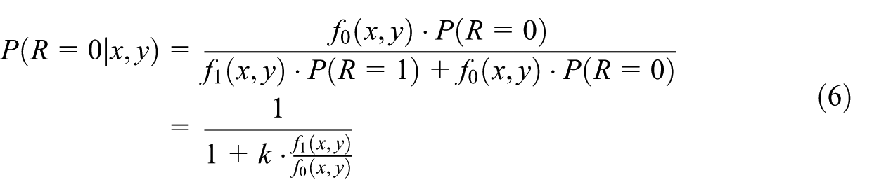
where and denote the two bivariate normal densities (for and , respectively), and . By using this formulation, the PPMM can be expressed as a selection model to assist with the sensitivity analysis.
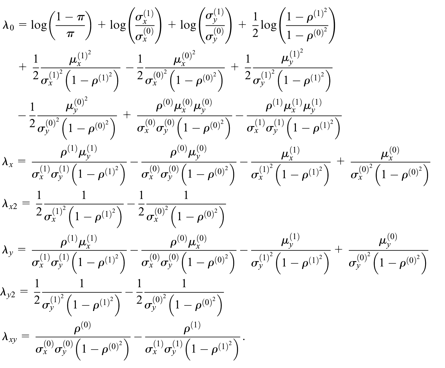
Starting from the Equation (6), applying the logit transformation to the nonresponse probability yields a quadratic form in and . The corresponding selection model implied by the PPMM defined in Equations (1) and (2) is thus
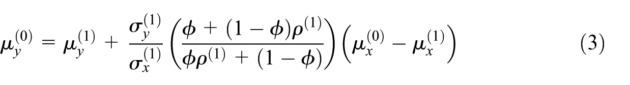
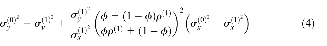
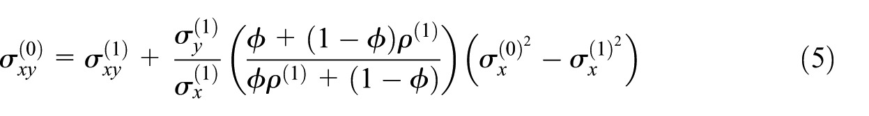
These formulas are expressed in terms of respondent and nonrespondent parameters and include parameters that are only identified via the assumption in Equation (2) (e.g., ). Plugging the formulas given in Equations (3) to (5) shows the parameters in terms of the sensitivity parameter (and parameters identifiable using observed data only). These resulting expressions are complex and not easily interpreted; the full expressions are shown in the online Supplemental Materials (Section A1).
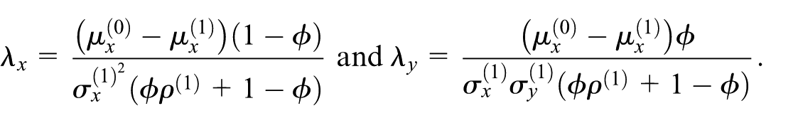
The corresponding selection model simplifies considerably when the respondent and nonrespondent proxy variances are equal, that is, . In this case, by Equations (4) and (5) we have and , and as a result, and the selection model is linear in and with no interaction term. The remaining nonzero coefficients reduce to the following closed-form expressions after plugging in the formulas given in Equations (3) to (5):
In this case, a single odds ratio, , describes the relationship between the outcome, , and the probability of nonresponse. This simplified expression reveals that the magnitude of the odds ratio for is a function of the standardized difference in proxy means between respondents and nonrespondents (, the strength of the proxy (), and the sensitivity parameter (). If the nonrespondent mean for is larger than the respondent mean, the odds ratio will be greater than one, which makes intuitive sense since is a proxy for . The correlation is in the denominator, such that smaller correlations—weaker proxies—will imply larger odds ratios. And when , as expected under an ignorable missingness mechanism.
When the respondent proxy variance is not equal to the nonrespondent variance, , , and are all non-zero. Thus the model is quadratic in both and and includes their interaction. The exception is when , in which case , , and are all zero (as expected with an ignorable nonresponse mechanism).
3.1. Visualization of the Corresponding Selection Model
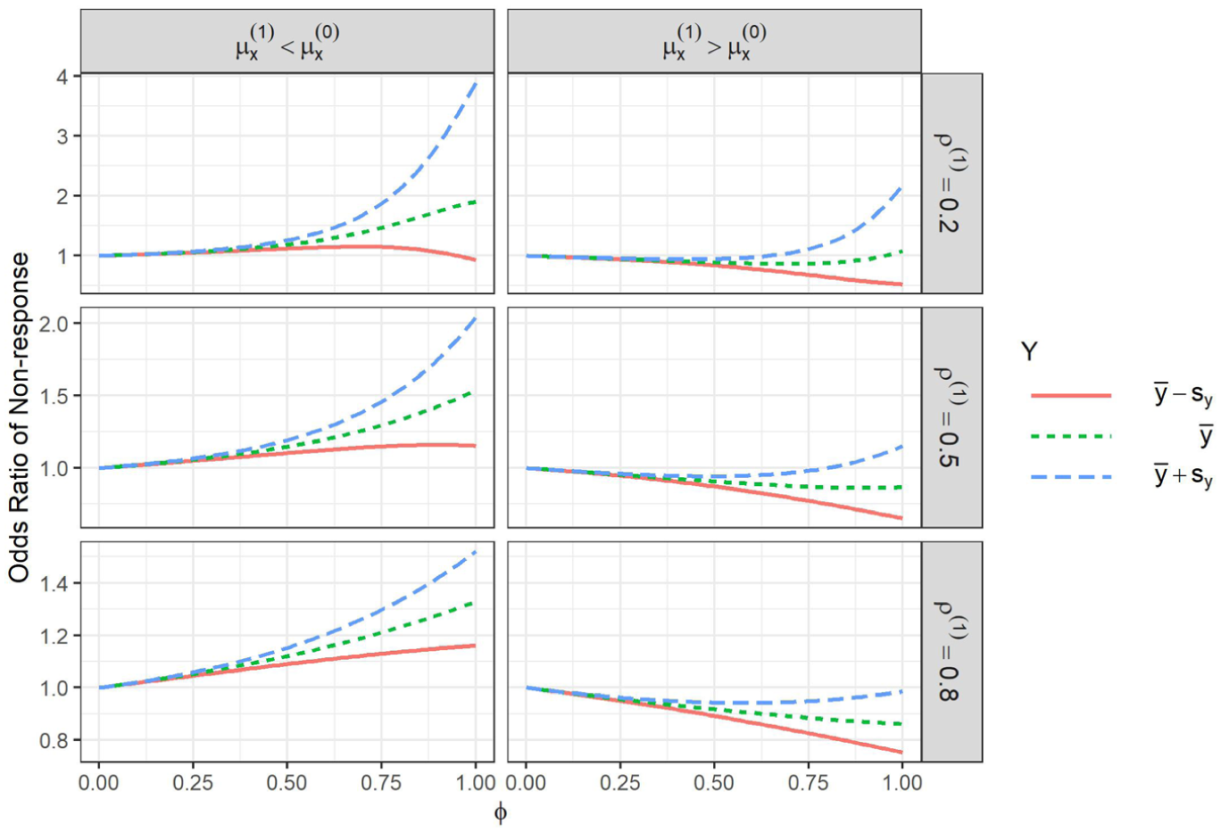
The selection model Equation (7) that corresponds to the PPMM can be difficult to understand due to the quadratic and interaction terms. Visualizing the results in terms of odds ratios can facilitate its interpretation. We computed the odds ratio of nonresponse for a unit increase in (based on Equation (7)) as a function of the sensitivity parameter for various combinations of the PPMM parameters. We considered a fixed response rate of . For respondents, we fixed the mean and variance of the proxy variable as well as the outcome at , but varied at to vary the strength of the correlation between the proxy and the survey outcome variable. We varied the nonrespondent mean and variance of the proxy at and respectively. We considered all the possible combinations of the varied parameters to obtain eighteen different mechanisms, that is, a factorial design.
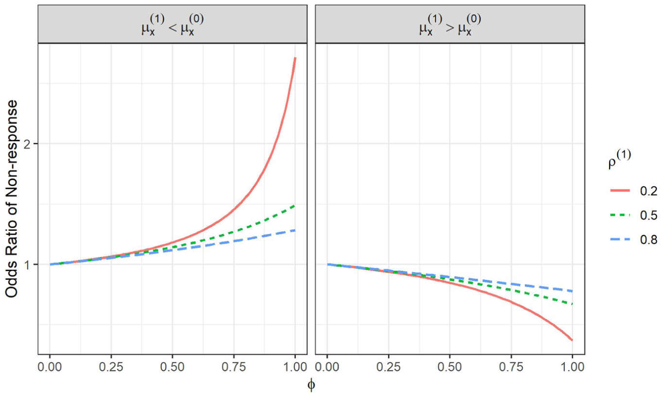
Figure 1 shows the selection model odds ratio for a unit increase in as a function of the sensitivity parameter for the cases when the respondent and nonrespondent proxy variances are equal. When , nonresponse is ignorable, so the corresponding odds ratio for is 1. The odds ratio moves away from 1 as increases, with the direction of the movement depending on whether the proxy mean is larger (left panel) or smaller (right panel) among nonrespondents. This makes sense, as larger values of correspond to missingness depending more strongly on . Importantly, for weaker proxies (smaller correlations), the odds ratio increases (decreases) at a more drastic rate. This illustrates a built-in assumption of the PPMM, that by definition weaker proxies will correspond to more severe missingness mechanisms (given similar proxy means and variances). However, even for the weakest proxy strength, the odds ratios are arguably not too unrealistic, as these odds ratio for a unit increase in , which is a one standard deviation increase, and the odds ratio only gets as large as approximately when .
Odds ratio of nonresponse for a 1 standard deviation increase in as a function of when . The proxy was fixed at its overall mean.
Figure 2 shows the selection model odds ratios for the cases when the respondent proxy variance is smaller than the nonrespondent proxy variance. In this case, the odds ratio for depends on and on itself due to the quadratic and interaction terms. Thus we computed odds ratios at three different values of (the respondent mean of plus/minus one standard deviation) and fixed the proxy at its overall mean.
Odds ratio of nonresponse as a function of when for different levels of : the respondent mean and 1 standard deviation below and above the respondent mean. The proxy variable was fixed at the overall mean of .
We see a similar pattern as in Figure 1 across all facets, with the odds ratio for nonresponse tending to increase in strength (move away from 1) as increases, with the rate of increment depending on the strength of the correlation. There is some evidence of potentially implausibly large odds ratios when approaches 1, particularly for weak proxies. In addition, in some instances the quadratic relationship causes some undesirable results for large values. For example, in the upper left panel of Figure 2, when is one standard deviation below its mean (red line), the odds ratio initially increases as a function of but then starts to decrease, eventually crossing one when is approximately 0.9. This implies that, for close to 1, increasing is associated with decreased odds of nonresponse—the opposite of what might be expected and what the rest of the plot shows. This information could inform a more tight bound on for a sensitivity analysis, excluding the values that lead to this type of selection mechanism.
When the respondent proxy variance is greater than the nonrespondent variance, similar patterns are observed (Supplemental Figure A1). Odds ratios are slightly larger and the direction of curvature is flipped between the smaller and larger values of .
We also examined the odds of nonresponse at other values of , including one standard deviation below and above its mean. These additional analyses showed that changing the value of primarily results in slight shifts in the odds ratio curves, while the overall patterns and sensitivity to remain unchanged. Plots for these other values of are included in the Supplementary Materials (Figure A2).
4. Application to Home Pricing Data
In order to see how the re-expressed PPMM as a selection model could inform a sensitivity analysis, we analyzed home pricing data previously analyzed in the context of nonignorable nonresponse by Miao et al. (2024). The home pricing dataset was extracted from the China Family Panel Studies and collected from 3,126 households in China. The outcome of interest is log of current home price (in RMB yuan), of which 597 (19.1%) values are missing, because the house owner did not respond in the survey, nor is the price available from the real estate market. Completely available covariates include province, urban (1 for urban household, 0 for rural), travel time to the nearest business center, house building area, family size, house story height, log of family income, and refurbish status.
The China Family Panel Studies dataset provides survey weights; however, survey weights were not used in this analysis. Our focus is on modeling and adjusting for nonresponse within the observed sample, rather than on population-level inference. As such, incorporating survey weights is not required for the methodological objective of this application and would not directly affect the nonresponse mechanisms under study. This choice is consistent with the application in Miao et al. (2024), which also did not incorporate survey weights.
We created the proxy for the log-transformed current home price, using a linear regression model with the main effects of all completely available covariates listed above as predictors. The resulting correlation between the proxy () and the outcome variable (log-transformed current home price) among respondents was , and the respondent proxy mean () and variance () were greater than the corresponding values for nonrespondents (). Graphs confirmed both the outcome variable (log-transformed current home price) and the proxy variable, were approximately normally distributed (Supplemental Figure A3).
4.1. Results
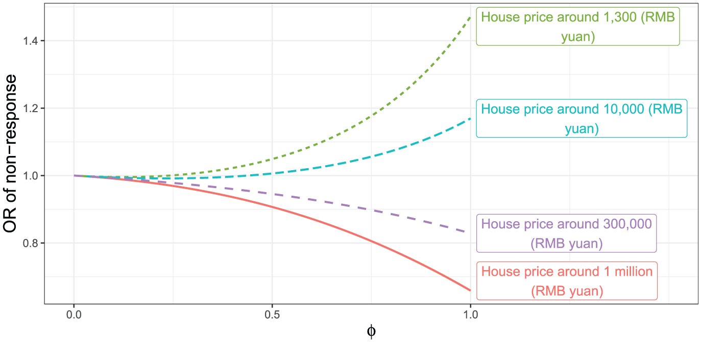
Figure 3 shows the odds ratio of nonresponse for a one-unit increase in (log-transformed current home price) as a function of for various values of , with the proxy fixed at its mean. The curves show how the strength and direction of the association between home price and survey nonresponse vary under different assumptions about the selection mechanism. For higher home prices, for example, when the home price corresponds to approximately 1 million RMB yuan or 300,000 RMB yuan, the odds ratio decreases below one as increases. This indicates that households with more expensive homes become increasingly less likely to be nonrespondents when the missingness mechanism depends strongly on the outcome. In other words, under stronger outcome-dependent selection mechanism, higher home prices are associated with a greater likelihood of responding. In contrast, for lower values of home price (e.g., approximately 1,300 RMB yuan), the odds ratio rises above one as increases, indicating that households with lower-priced homes are increasingly likely to be nonrespondents when the selection mechanism depends more strongly on the outcome. This suggests that nonresponse is not uniform, but instead varies across the home price distribution, with lower-value properties being more frequently unreported, possibly due to privacy concerns, stigma, or discomfort disclosing asset information. In both directions, the rate of increment or decrement depends on the value of the home price since the selection model is quadratic in . The odds ratio increases or decreases more rapidly as a function of for higher or lower home prices respectively.
Odds ratio of nonresponse (for a +1 unit increase in log of current home price in RMB yuan) as a function of for different levels of the outcome variable (log of current home price in RMB yuan) with the proxy variable fixed at its overall mean.
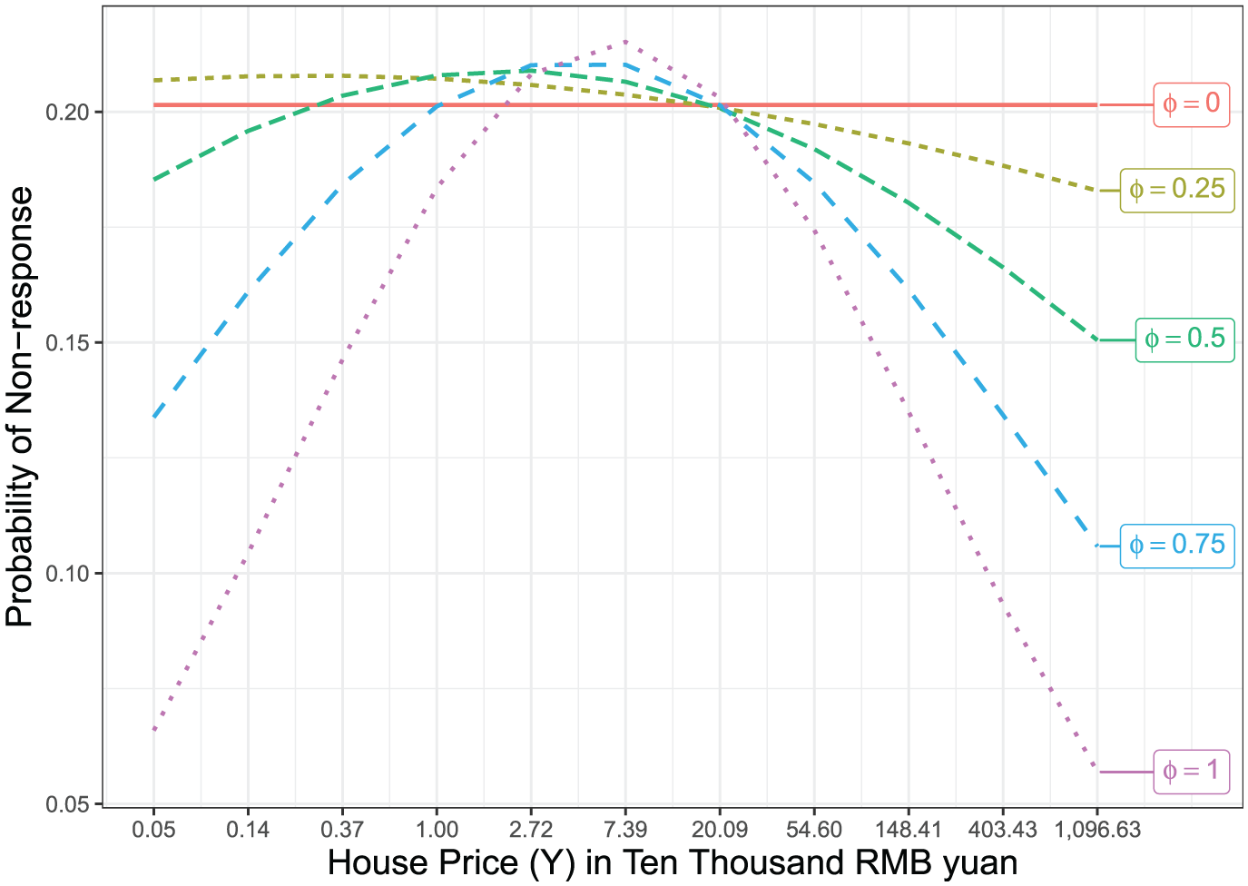
We can also visualize the implied probability of nonresponse for the log-transformed current home price as a function of its value, derived from the logistic selection model under varying levels of the sensitivity parameter, . Figure 4 shows the probability of missing home price as a function of home price for different values of . As expected, when , the missing data mechanism is ignorable and the probability of nonresponse is constant across all values of house price. However, for , the relationship becomes distinctly non-monotonic: the probability of nonresponse peaks near the center of the house price distribution and declines for both low and high values of house price. This bell-shaped curvature becomes more pronounced as increases. Notably, for , the implied probability of missingness is very low (approximately 6%–7%) for both expensive homes and very inexpensive homes. These patterns suggest that the likelihood of reporting house price is highest at the extremes of the distribution and lowest around the middle, under strong selection/missingness mechanism. One possible interpretation is that households with very high home prices may be more comfortable disclosing this information, perhaps due to social standing or confidence in property value. On the other hand, those with moderately priced homes may be more uncertain or reluctant, potentially due to market fluctuations or perceived judgment. At the lower end, while some nonresponse may be expected due to stigma or privacy, the probability of missingness appears to level off or even decline as increases, possibly indicating reduced sensitivity for these households under strong selection/missingness assumptions.
Probability of nonresponse as a function of the outcome, log of current home price in RMB yuan, for different levels of the sensitivity parameter , with the proxy variable fixed at its mean in the full data. The x-axis is on the log-scale but labeled on the original scale.
Interestingly, the estimated overall median home price (in RMB yuan) under the PPMM does not vary much as a function of . The respondent median home price is 15.318, and the PPMM estimates only range from 14.984 for to 14.806 for (see Supplemental Figure A4). This is despite the difference in proxy means between respondents and nonrespondents (approximately 0.1 standard deviations). This is a direct consequence of the quadratic selection mechanism; under the PPMM as applied to the housing price data, both larger and smaller values become increasingly less likely to respond, essentially canceling each other out in terms of impact on the overall mean. Understanding that the PPMM implies this quadratic relationship helps explain this possibly surprising result.
5. Discussion
In this paper, we have explored the equivalence and application of proxy pattern-mixture models (PPMM) in a selection model framework to help judge the magnitude of nonignorable missingness or selection under the PPMM. The integration of these two models helps translate the PPMM sensitivity parameter into a potentially easier to interpret odds ratio, and can potentially facilitate a sensitivity analysis by suggesting tighter bounds on . The selection model that corresponds to the proxy-pattern mixture model is a quadratic function of the survey outcome () and proxy variable (). However, the magnitude of the quadratic effect depends on the strength of the proxy (i.e., how well the covariates predict the survey outcome among respondents) with more severe quadratic effects for weaker proxies. Having access to strong predictors of the survey outcome of interest has previously been suggested as important for the PPMM (e.g., Little et al. 2020) and our analysis reveals that in fact the effect of on response can sometimes be implausible under the PPMM with weaker covariates (e.g., effects changing direction).
Regardless of the strength of the proxy, our results show that the odds ratio for becomes exaggerated for values close to one. This can lead to unrealistic or extreme estimates of the nonresponse mechanism, highlighting the need for careful selection and justification of the choice of for a sensitivity analysis. This selection model formulation suggests that for many scenarios we might want to place an upper bound on the sensitivity parameter that is smaller than .
An alternative approach to assessing the plausibility of various values would be to perform imputation under the PPMM and evaluate the resulting imputed values. Imputing under the PPMM for a fixed value of is straightforward (see Andridge and Little (2011) for details) and several types of evaluations could be done using the imputations. For example, one could use domain knowledge to identify at what value the marginal and/or conditional distributions of the imputed values become implausible (e.g., imputed values are impossibly large). We see such an approach as a complementary approach to the odds ratio approach, providing a different view of the implied “magnitude” of the nonresponse mechanism and its impact on estimates.
Our results directly extend to the PPMM for binary outcomes (Andridge and Little 2020; Andridge et al. 2019). The binary PPMM assumes that is related to a normally distributed latent variable through the rule that when the latent variable . The corresponding selection model is identical to (7), substituting in place of . The only difference is that since is a latent variable, we cannot estimate both its mean and variance for the respondents, and thus the variance component for the respondents is fixed at for latent variable (i.e., ). We emphasize, however, that the corresponding odds ratios from the selection model are for the latent variable underlying the binary outcome , not for itself, and thus may be challenging to interpret.
We note that our analysis adopts a frequentist sensitivity framework in which the sensitivity parameter is varied over a fixed range. An alternative approach would be to use a Bayesian framework to place a prior distribution on the sensitivity parameter, as suggested in previous work (Andridge et al. 2019; Little et al. 2020). This would allow uncertainty about the sensitivity parameter to be incorporated directly into the analysis and would yield a posterior distribution for the odds ratio of , providing an alternative way to summarize sensitivity to departures from ignorability.
The PPMM framework itself can be applied under a wide range of outcome distributions, including settings where the target variable is skewed or multimodal (Andridge and Thompson 2015a). However, the specific selection model interpretation developed in this paper and the resulting odds ratio interpretation relies on the assumption that the target variable and the corresponding proxy are normally distributed. Importantly, this normality requirement applies to the outcome and proxy variables, but not to the covariates used to construct the proxy, which may be skewed or have complex distributions. In our data application, exploratory analyses (Supplemental Figure A3) indicated that both the outcome and proxy were close to normal, supporting the use of this interpretation. When outcome or proxy distributions have non-normal distribution, such as substantial skewness, heavy tails, or bimodality, the results described in this paper do not hold, and the PPMM cannot be expressed as a logistic regression model. In these cases, alternative PPMM formulations may be applicable but the connection to an odds ratio via a selection model is lost.
Another feature of the PPMM framework is that, although surveys typically collect multiple related outcome variables under a common response or selection process, the model is applied one outcome at a time. In its current form, PPMM assesses the potential impact of nonresponse or selection on the mean of a specific survey outcome, Y without explicitly accounting for associations with other outcomes measured in the same survey. As most surveys have multiple target variables, extensions of the approach to jointly model multiple outcomes under a shared nonresponse or selection mechanism could potentially be useful and is a consideration for future work. One such an approach could be to create proxies based on covariates for each of several outcome variables and jointly model them with the outcomes via a multivariate pattern-mixture model (Little and Wang 1996). However, this more complex model would at a minimum require separate sensitivity parameters for each outcome, thus complicating both interpretation and implementation. Nonetheless, this is an interesting area for future work.
In some applications, data may be collected under multiple survey designs or modes, each potentially giving rise to a different selection mechanism while sharing common underlying factors related to participation. The PPMM framework considered in this paper could be separately applied to different data collection efforts (e.g., experiments embedded in an ongoing survey) and could potentially be used to monitor data quality. Wagner (2010) suggested using the fraction of missing information as a metric for this purpose; the odds ratio for under the PPMM could be used to compare across designs in a similar fashion. This would potentially allow insight into which design or mode had a larger potential for nonignorable nonresponse bias (under the assumptions of the PPMM). Evaluation of how the PPMM and corresponding odds ratio interpretation could be used in this context is an area for future work.
Another area for future research is the use of this selection model expression of the PPMM to obtain nonignorable nonresponse propensities for given values of . This could enable the construction of inverse propensity weights under various degrees of nonignorable nonresponse. This may provide a straightforward way to estimate subgroup effects under the PPMM, which in its current form requires reapplying the method with subsets of data and, in the case of application of the PPMM to selection issues, separate population-level aggregate information on the subset, which might not be readily available. Our results therefore provide a basis for the development of nonignorable weights to adjust for potential biases introduced by the relationship between the survey outcome and nonresponse.
Supplemental Material
sj-pdf-1-jof-10.1177_0282423X261457501 – Supplemental material for Re-Expressing the Proxy Pattern-Mixture Model as a Selection Model to Assist with Sensitivity Analysis
Supplemental material, sj-pdf-1-jof-10.1177_0282423X261457501 for Re-Expressing the Proxy Pattern-Mixture Model as a Selection Model to Assist with Sensitivity Analysis by Seth Adarkwah Yiadom and Rebecca Andridge in Journal of Official Statistics
Footnotes
Appendix 1
Let and denote two bivariate normal densities with different parameters. The general form of the bivariate normal density is:
where the quadratic form is given by:
for .
The PPMM assumes a bivariate normal distribution for the joint distribution of conditional on the response indicator . By restricting the two joint distributions when and to be normal, the implied response mechanism naturally takes the form of a logistic function:
where and denote the two bivariate normal densities, and . Similarly,
Applying the logit transformation to the nonresponse probability yields
The authors disclosed receipt of the following financial support for the research, authorship, and/or publication of this article: This work was supported by a grant from the National Institutes of Health (R03CA280007; Principal Investigator Andridge).
ORCID iDs
Seth Adarkwah Yiadom
Rebecca Andridge
Supplemental Material
Supplemental material for this article is available online.
Received: September 22, 2025
Accepted: May 6, 2026
References
1.
AndridgeR.ThompsonK. J.2015a. “Assessing Nonresponse Bias in a Business Survey: Proxy Pattern-Mixture Analysis for Skewed Data.” The Annals of Applied Statistics9 (4): 2237–65. DOI: 10.1214/15-AOAS878.
2.
AndridgeR.ThompsonK. J.2015b. “Using the Fraction of Missing Information to Identify Auxiliary Variables for Imputation Procedures Via Proxy Pattern-Mixture Models.” International Statistical Review83 (3): 472–92. DOI: 10.1111/insr.12091.
3.
AndridgeR. R.2024. “Using Proxy Pattern-Mixture Models to Explain Bias in Estimates of Covid-19 Vaccine Uptake from Two Large Surveys.” Journal of the Royal Statistical Society Series A: Statistics in Society187 (3): 831–43. DOI: 10.1093/jrsssa/qnae005.
4.
AndridgeR. R.LittleR. J.2011. “Proxy Pattern-Mixture Analysis for Survey Nonresponse.” Journal of Official Statistics27 (2): 153.
5.
AndridgeR. R.LittleR. J.2020. “Proxy Pattern-Mixture Analysis for a Binary Variable Subject to Nonresponse.” Journal of Official Statistics36 (3): 703–28. DOI: 10.2478/jos-2020-0035.
6.
AndridgeR. R.SongR.WestB. T.2025. “A Sensitivity Analysis Framework Using the Proxy Pattern-Mixture Model for Generalization of Experimental Results.” Statistics in Medicine44 (25–27): e70313. DOI: 10.1002/sim.70313.
7.
AndridgeR. R.WestB. T.LittleR. J.BoonstraP. S.Alvarado-LeitonF.2019. “Indices of Non-Ignorable Selection Bias for Proportions Estimated from Non-Probability Samples.” Journal of the Royal Statistical Society Series C: Applied Statistics68 (5): 1465–83. DOI: 10.1111/rssc.12371.
8.
BoonstraP. S.LittleR. J.WestB. T.AndridgeR. R.Alvarado-LeitonF.2021. “A Simulation Study of Diagnostics for Selection Bias.” Journal of Official Statistics37 (3): 751–69. DOI: 10.2478/jos-2021-0033.
9.
GlynnR. J.LairdN. M.RubinD. B.2013. “Selection Modeling Versus Mixture Modeling with Nonignorable Nonresponse.” In Drawing Inferences from Self-Selected Samples, edited by H.Wainer. Routledge. DOI: 10.1007/978-1-4612-4976-4_10.
10.
HammonA.ZinnS.2024. “Validating an Index of Selection Bias for Proportions in Non-Probability Samples.” International Statistical Review93 (3): 499–516. DOI: 10.1111/insr.12590.
11.
JacksonM.2023. “Can New Metrics Help Us Get a Handle on Partisan Nonresponse Bias? Evidence from State-Level 2022 Polling.” 78th Annual AAPOR Conference. AAPOR. Philadelphia Marriott Downtown. May 12, 2023.
12.
KacirotiN. A.RaghunathanT.2014. “Bayesian Sensitivity Analysis of Incomplete Data: Bridging Pattern-Mixture and Selection Models.” Statistics in Medicine33 (27): 4841–57. DOI: 10.1002/sim.6302.
13.
LittleR. J.WangY.1996. “Pattern-Mixture Models for Multivariate Incomplete Data with Covariates.” Biometrics52 (1): 98–111. DOI: 10.1080/01621459.1993.10594302.
14.
LittleR. J.WestB. T.BoonstraP. S.HuJ.2020. “Measures of the Degree of Departure from Ignorable Sample Selection.” Journal of Survey Statistics and Methodology8 (5): 932–64. DOI: 10.1093/jssam/smz023.
15.
MiaoW.LiuL.LiY.TchetgenE. J.GengZ.2024. “Identification and Semiparametric Efficiency Theory of Nonignorable Missing Data with a Shadow Variable.” ACM/JMS Journal of Data Science1 (2): 1–23. DOI: 10.1145/3592389.
16.
WagnerJ.2010. “The Fraction of Missing Information as a Tool for Monitoring the Quality of Survey Data.” Public Opinion Quarterly74 (2): 223–43. DOI: 10.1093/poq/nfq007.
17.
WestB. T.AndridgeR. R.2023. “Evaluating Pre-Election Polling Estimates Using a New Measure of Non-Ignorable Selection Bias.” Public Opinion Quarterly87 (SI): 575–601. DOI: 10.1093/poq/nfad018.
18.
WestB. T.LittleR. J.AndridgeR. R., et al. 2021. “Assessing Selection Bias in Regression Coefficients Estimated from Nonprobability Samples with Applications to Genetics and Demographic Surveys.” The Annals of Applied Statistics15 (3): 1556. DOI: 10.1214/21-aoas1453.
19.
YangY.LittleR. J.2021. “Spline Pattern-Mixture Models for Missing Data.” Journal of Data Science19 (1): 75–95. DOI: 10.6339/21-JDS1008.
Supplementary Material
Please find the following supplemental material available below.
For Open Access articles published under a Creative Commons License, all supplemental material carries the same license as the article it is associated with.
For non-Open Access articles published, all supplemental material carries a non-exclusive license, and permission requests for re-use of supplemental material or any part of supplemental material shall be sent directly to the copyright owner as specified in the copyright notice associated with the article.