Continuous self-report engagement responses to the live performance of an atonal,post-serialist solo marimba work

Abstract

Repetition of musical sections, tempo, and physical sound intensity associate strongly with listeners’ affective responses to tonal music in controlled laboratory studies. What contribution might repetition, temporal and acoustic variables make to observers’ responses where music lacks a diatonic tonal structure, an obvious beat, and is performed live? The present study investigates relationships between musical repetition (motivic cells and phrases), note density (sequentially occurring), and intensity with observers’ continuous self-report ratings of engagement with an unfamiliar, atonal post-serialist solo marimba work performed live. Following training, 19 audience members continuously self-reported engagement on a bi-polar, one-dimensional scale using the portable Audience Response Facility. Note density and intensity contributed significantly (or explained variance) to observer engagement with the performance. Contrary to expectation, the repetition variables did not contribute significantly. Controlling serial correlation using a new modelling approach based on Box–Jenkins ARIMA transfer modelling, density emerged as the prime contributor to observer engagement. A single performance appeared to provide observers with insufficient exposure to understand and respond to the structure of atonal music. Note density potentially enabled observers to segment the musical surface and develop some structural understanding, possibly underpinned by stimulus-driven entrainment processes shaping attentional behaviour and musical expectations.

Keywords

atonal music intensity music performance musical repetition note density observer engagement time-series analysis

Composers structure musical elements to engage audience members’ attention, and elicit cognitive and emotional responses to the artistic performance of the work. The repetition and development of musical ideas is a key technique to structure music (e.g., theme and variations, or ternary form – ABA). Considering Western classical music from the 17th to 19th centuries, Kivy (1993, p. 352) argued that musical repeats “perform an obvious and vital function in that they are the composer’s way of allowing us, indeed compelling us to linger; to retrace our steps so that we can fix the fleeting sonic pattern; they allow us to grope so that we can grasp”. Current thinking in music, cognitive psychology and neuroscience disciplines supports the notion that repetition is important in how listeners respond to, engage with, and understand music of various genres and times (Margulis, 2014). Within this frame, the present study investigates the role that musical repetition plays in engagement with the live performance of a post-modern, atonal post-serialist solo marimba work.

Repeated exposure in developing listeners’ or observers’ understanding of music structure

Musical repetition assists listeners in developing some understanding of the structuring and sequencing norms of the music. Mere exposure to repeated stimuli is sufficient to develop individuals’ preference for the stimuli encountered, even if the individual is not consciously aware of the exposure (Zajonc, 1968, 2001). Through exposure to the music of a culture, such as Western classical art music, musically untrained listeners demonstrate some music capacities that are similar to those with greater musical experience and training (Bigand & Poulin-Charronnat, 2006). Through exposure, musically trained and untrained listeners can recognise, extract grammatical information from, and have preference for repeated melodies constructed from an artificial grammar (Loui, Wessel, & Hudson Kam, 2010). Within an experimental session, listeners can acquire incidentally structural knowledge about melodic sequences created using an artificial grammar (Rohrmeier, Rebuschat, & Cross, 2011), or develop familiarity with, and learn the structure of, culturally unfamiliar music (Stevens, Tardieu, Dunbar-Hall, Best, & Tillmann, 2013). Audience members’ continuous psychophysiological affective responses to live performances appear to be shaped by musical expectations, which are proposed to develop through statistical learning about the often hierarchical organisation of pitches and musical segments (Egermann, Pearce, Wiggins, & McAdams, 2013). In sum, listeners (audio-only musical exposure) or audience members (hence observers, indicating seeing and hearing music performance) should develop some familiarity with and understanding of the structure of an unfamiliar musical work from exposure to repeated musical elements through the performance.

Listeners’ overt, cognitive judgments demonstrate sensitivity to the structure of Western tonal music, but not atonal music. Western tonal music uses diatonic scales, and features a hierarchy of tonal relations (Bharucha & Krumhansl, 1983; Krumhansl & Kessler, 1982; Lerdahl & Jackendoff, 1983). The particular way in which tones and rhythmic values are combined determines patterns of tension and relaxation in tonal music phrases (Bigand, 1993). Listeners appear to be sensitive to these patterns, as shown where repeated music sections or phrases attract similar continuous self-report judgments of experienced tension (Krumhansl, 1996) and perceived arousal (Livingstone, Palmer, & Schubert, 2012). In atonal music usually no pitches are more or less closely related than others and a hierarchic structure similar to that of Western tonal music appears not to exist (Dibben, 1994). In an experiment using extracts of two pieces of atonal music and different reductions of each extract, Dibben (1994) reports that listeners were unable to correctly match reductions that were more similar to the extracts in their underlying structure, than less similar reductions. If listeners are unable to grasp the underlying tonal structure in atonal music, repeated exposure to units of music (e.g., collections of pitch sequences) within the piece might help listeners to discern more from less similar units, and build some understanding of the music structure.

Cognitive processes implicated in listeners’ or observers’ responses to musical repetition in music performance

Perceptual similarity has been proposed as an important feature of how music is processed and understood. From a cognitive psychology perspective, cue abstraction theory proposes that listeners are able to abstract from the musical surface musical features (cues), which form the basis of hierarchically organised mental schemata (Deliège, 1996, 2001; Deliège, Mélen, Stammers, & Cross, 1996). Deliège (2007) argues that similarity plays a central role in segmenting the musical surface into more manageable chunks, or units, to process. Certain characteristics of the music, such as melodic pitch leaps, contribute to perceptual similarity and implicit formation of prototype category processes for musical motifs or segments, which, in turn, underpin representations of musical style, structure, or features of the composer’s language (Deliège, 2007). Cambouropoulos (2009) highlights that similarity and categorisation are related, and crucially, that judgments regarding perceptual similarity and categorisation are dependent on the context in which they are made. From a music theory perspective, Hanninen (2003) highlights the importance of context to the abstraction and interpretation, or “recontextualization”, of musical ideas. Musical segments, ideas, or “things” are not only abstracted from a musical context, but also crucially related to the context in which they exist. Therefore, listeners might perceive musical ideas that exist in different musical contexts within a piece as repetition or transformation of the idea. While the present study does not examine these theoretical propositions explicitly, the idea that repetition, based on the musical similarity of segments, contributes to listeners’ responses to and understanding of the structure of music is relevant. Moreover, the surface features of the music, rather than the underlying structure, could provide listeners with the most efficacious way of engaging with unfamiliar music.

Previous research indicates that listeners are sensitive to similarity between relatively short-duration repeated musical units (from a motif to a phrase), even where there is intervening musical material. Margulis (2013) reports that immediate or delayed musical repetition increased listeners’ enjoyment and artistry ratings for excerpts of atonal 20th-century classical art music (adapted to include repetition), in comparison to the original excerpts. Whether tone sequences are temporally adjacent or nonadjacent, perceptual similarity appears to play an important role in how listeners learn the statistical regularities in melodic tone sequences (Creel, Newport, & Aslin, 2004). However, repeated units in tonal music might be best detected when they are immediately adjacent, approximately 6 s in duration, occurring within a phrase, and when a complete unit is repeated; over multiple exposures, listeners appear to shift attention from short to long units of music (Margulis, 2012). In short, within a single performance, or exposure, similarity between musical units, effected through musical repetition, is reflected in listeners’ cognitive, aesthetic and affective responses. Furthermore, musical repetition seems to stimulate listeners’ attention to and cognitive processing of the music structure in different ways.

Observers engage working and long-term memory as they respond to live music performance. For example, McAdams, Vines, Vieillard, Smith, and Reynolds (2004) gathered observers’ continuous self-report familiarity/resemblance and emotional force responses to the live performance of an unfamiliar contemporary electroacoustic music work (composed for solo piano, chamber orchestra, and computer-processed sonic material – see Reynolds, 2004). Working memory processes were implicated where matched changes in the unfurling sensory information and observers’ familiarity/resemblance responses were observed – taken to reflect an underlying process of comparing sensory information to that held in working memory. Observers’ responses changed at section boundaries where there was a change to the musical material or texture. An increase or decrease in observers’ familiarity/resemblance responses to previously heard or unheard thematic materials respectively indicated long-term memory processes. Interestingly, only some core elements of thematic material (core element referred to the most important subsection of a particular theme for the theme’s progression) appeared to be recognised implicitly. Changes in instrumentation impaired recognition of core elements (Poulin-Charronnat et al., 2004). McAdams et al. (2004) found that while observers’ emotional force ratings generally decreased over the course of the concert, they increased in response to certain sections of the music – particularly those comprising computer-generated sounds, which featured increasing sonic density and intensity. Familiarity and emotional force ratings followed similar patterns in some places, indicating shared relations to the music structure, but diverged in others. In sum, results suggested that observers glean information about structure of unfamiliar music through exposure during performance, and this is reflected in their overt cognitive and affective responses. Additionally, elements of the musical surface, such as timbre, sonic density and intensity, and change in musical material, appeared to shape observers’ responses in the moment. Therefore, where an unfamiliar musical work is performed on a single instrument, hence presenting a single timbral category, might musical repetition, and sonic density and intensity acoustic variables play an important role in observers’ engagement with the performance experience?

The influence of acoustic variables on judgments of music performance

The pace at which music is performed, usually referred to as tempo, has been shown to influence listeners’ affective responses to music. Generally speaking, increases in tempo are matched by the music being judged increasingly as happy (cf. slow tempo and sad; Gagnon & Peretz, 2003; Webster & Weir, 2005), and this association is present from about the age of five years (Dalla Bella, Peretz, Rousseau, & Gosselin, 2001). Fast tempo music is also judged as more arousing (Balch & Lewis, 1996; Husain, Thompson, & Schellenberg, 2002). Furthermore, Husain et al. (2002) report that enjoyment, as well as arousal, is sensitive to tempo manipulation, especially when music is in a major key, or mode. Although the effect of mode (i.e., major versus minor) on listener judgments is probably less relevant to the present study, the notion that there is a positive association between tempo and enjoyment is highly relevant.

In the present study, note density (density – the number of sequential sound onsets within a defined time frame) is used as a predictor of observer engagement responses. Note density is used as a temporal measure of the music as it is unclear from previous research what exactly constitutes a fast and slow tempo. For example, in the aforementioned studies, slow tempo ranges from 60 (Balch & Lewis, 1996; Husain et al., 2002) through to 72 (Webster & Weir, 2005) and even 110 beats per minute (bpm; Gagnon & Peretz, 2003). Similarly, fast tempo ranges from 140 (Balch & Lewis, 1996), to 144 (Webster & Weir, 2005), 165 (Husain et al., 2002), up to 220 bpm (Gagnon & Peretz, 2003). An overarching measure of tempo, such as bpm, may not correspond optimally to the temporal patterning of music to which observers most readily respond. Rather than the musical stimuli’s absolute bpm, the relationship perceived between different tempi may be an important influence on listeners’ responses to the music. Note density might be a relevant measure since observers actually hear the different inter-onset intervals making up the varied temporal patterns of musical rhythm, rather an isochronous beat. Furthermore, an overarching temporal measure, such as bpm, does not consider that what might be perceived as fast music could be music of a slow bpm tempo, but featuring short-duration rhythms, or small inter-onset intervals, segmenting time.

Intensity often plays an important role in listeners’ affective responses to music. Several studies have demonstrated a link between perceived arousal and physical sound intensity, as an approximate measure of the perception of loudness (Bailes & Dean, 2012; Dean, Bailes, & Schubert, 2011; Schubert, 2004), and regardless of listeners’ familiarity with the music. However, other factors can mediate physical sound intensity measures and listeners’ affective responses to music. For example, listener engagement appears to mediate the relationship between acoustic, physically measurable, properties of music, such as intensity, and listeners’ affective responses to unfamiliar Western classical and electroacoustic music (Olsen, Dean, & Stevens, 2014). This relationship seems to rely on listeners’ consideration of the music as not too disliked or unfamiliar.

Observer engagement with live music performance

Observer engagement is measured in the present study to capture a range of elements contributing to observers’ responses to live music performance. Engagement is a term allied to motivation. According to Furrer and Skinner (2003), “engagement refers to active, goal-directed, flexible, constructive, persistent, focused interactions with the social and physical environments” (p. 149). Engagement involves cognitive, behavioural, and affective components (e.g., Furrer & Skinner, 2003; Reeve, Jang, Carrell, Jeon, & Barch, 2004; Russell, Ainley, & Frydenberg, 2005). In previous research in music contexts, engagement has been defined as compelled, drawn in, connected to what is happening in the music, interested in what will happen next (Olsen et al., 2014; Schubert, Vincs, & Stevens, 2013), and how engaged you are with the audio-visual performance experience (Broughton, Stevens, & Schubert, 2008). It is the latter definition that we use in this study, as previous research suggests that the concept of engagement in live performance contexts involves auditory and allied visual information. For example, results of a questionnaire suggest that the degree to which performers appear engaged in the performance contributes to observers’ attention to and enjoyment of music performance (Thompson, 2007). Similarly, performing in a projected manner (consistent with public performance; cf. deadpan manner where expression is minimised – see Davidson, 1993) appears to enhance observers’ continuous self-report engagement responses to live solo marimba performance (Broughton et al., 2008). In a live concert setting, the potential influence of visual information cannot easily be controlled. However, it is arguably of interest for musicians and researchers alike to better understand how audience members engage with music performance in authentic contexts (see Burland and Pitts, 2014).

Aim and research questions

The present study investigates relationships between musical repetition, note density, physical sound intensity, and observers’ continuous self-report responses of engagement with an unfamiliar, atonal post-serialist solo marimba work performed live. Musical repetition, note density, and sound intensity variables are expected to associate positively with engagement ratings. We also expect that the engagement response data feature a time-dependent, serially correlated component due in part to the close temporal proximity of consecutive samples. However, our primary interest is to investigate the contribution of musical repetition, note density and sound intensity elements to engagement ratings beyond time-dependent, serial processes. While these variables most likely interact in music in varying manners, our interest is to understand whether they contribute to observer engagement with authentic, intact music performed in a live concert context, rather than music created with experimental controls for the study.

Method

Participants

Participants, or observers, were recruited via a convenience sample from those attending the HCSNet SummerFest ’06 in Sydney, and others who responded to external advertising for the concert. Twenty-three observers, in a total audience of approximately 100, took part in the study. Data from four observers were omitted: one - a percussionist - because of possible familiarity with the music and marimba playing techniques; another as she/he was not performing the task required – she/he was doodling or “skywriting” (Lucas, Schubert, & Halpern, 2010); two showed no variation, possibly indicating technical error. Of the remaining 19 observers, seven were female (mean age = 33.00 years, SD = 11.79), and 12 were male (mean age = 32.17 years, SD = 7.86). Twelve observers self-reported six or more years of formal music training, and were active in performing, composing, or teaching music. They were classified as “musically trained” for the purpose of this study (mean years training = 13.17, SD = 6.94). The musically untrained observers numbered seven (all reporting no music training). Participation was dependent on self-reported normal, or corrected-to-normal, vision and hearing.

Stimuli and equipment

The first movement of The Source for Solo Marimba by Toshi Ichiyanagi (1991) served as the stimulus material (duration 4 min 46 s). Researcher MCB performed the solo marimba work approximately 40 minutes into a 50-minute concert at Sancta Sofia College, University of Sydney. The performance venue was a large room used for chamber music concerts, set with rows of chairs facing the performance area. The performer was dressed in predominantly black concert clothing. The music was performed on a Malletech Stiletto five-octave marimba.

Observers’ continuous self-report engagement (how engaged you are with the audio-visual performance experience, Broughton et al., 2008) was recorded using the portable Audience Response Facility (pARF, Stevens, Schubert, Haszard Morris et al., 2009). Previous research has successfully employed this methodology (e.g., Broughton et al., 2008; Egermann et al., 2013; McAdams et al., 2004; Olsen et al., 2014; Schubert et al., 2013), and reported that performing such a task does not interfere greatly with observers’ responses to the music performance stimuli (Egermann et al., 2013; Stevens, Vincs, & Schubert, 2009). In an evaluation study of the portable Audience Response Facility (pARF) – the system used in the present study – Stevens, Vincs, and Schubert (2009) concluded that using the device to respond to live performance placed relatively small cognitive and attentional demands on observers. Following training, we expected that observers would be able to use the pARF to perform the research task as requested.

The pARF consisted of palm-sized client devices featuring a touch-sensitive screen on which observers drew with a pen-like object called a stylus. Each client device was connected wirelessly to a server. The client device was an HP iPAQ Pocket PC h5500 with an Intel PXA255 processor and 128MB of memory running Microsoft Pocket PC version 4.20.0. The screen size measured 240 x 480 pixels. Engagement was measured on the x-axis of the screen; the scale ranged from not engaged (–120 px) – neutral (0 px) – engaged (+120 px). Observers’ responses were sampled at a frequency of 2 Hz by recording the pixel position at which the stylus made contact with the client-device screen. The client devices connected to the server via an 802.11 Wi-Fi network. The server was an Acer TravelMate 8000 laptop computer with a 1.8 GHz Pentium M processor and 1 GB of memory, running Microsoft Windows 2003. The server stored study information including observers’ response data. Prior to commencement of the concert, the pARF server sent synchronisation packets to the client devices to synchronise them with the server clock.

A digital video recording of the live performance and the server clock was made to enable timecode matching of the response data to the performance. The digital video camera used was a Sony HandyCam HCR-30E recording 25 frames per second. A digital 48 kHz 24-bit audio recording was also made using two matched Neumann KM140 condenser microphones and the ORTF stereo recording technique (17 cm apart, 110 degree angle). The performance was recorded on a PowerBook Mac computer running ProTools version 6.9 using a Digidesign Digi 002 interface connected via FireWire. The 48 kHz 24-bit AIFF file format was converted to 44.1 kHz 16-bit format in QuickTime 7.1. The digital video (.avi) and audio (.wav) files of the recorded performance were synchronised and edited in Adobe Premier Pro 1.5. Physical sound intensity values were extracted from the .wav file using PRAAT version 4.6.01 by running an overall intensity script with a sampling rate of 2 Hz. The spectrum display in Audacity version 1.2.5 was used in determining note density scores in conjunction with the music score and sound recording.

Procedure

Observers arrived 30 minutes prior to the commencement of the concert. After obtaining written informed consent, they were directed to a quiet room adjacent to the concert venue. Here observers were given a questionnaire to complete gathering demographic and music background information. Then, in a 15-minute training session, observers were introduced to the pARF device and shown how to use it to make their engagement responses. They were instructed to keep the stylus in contact with the touch-sensitive screen throughout the duration of the concert, and move it across the screen to reflect their engagement. All observers reported being confident to perform the response task as required. Following training, observers were ushered into the concert venue, and seated in the first three rows, to stage right of the central aisle.

Observers made their continuous engagement responses during the various works performed in the 50-minute concert. Also on the concert programme was another solo marimba work, a duo for flute and marimba, a duo for horn and marimba, and a duo for horn and percussion. The performance of The Source for Solo Marimba (Ichiyanagi, 1991) was the final piece on the programme. Participants were able to rest between the various items in the concert. They had also the option to cease rating if they were tired, or wished to withdraw from the study. Participant responses to the first item on the programme, which was a tonal composition, were reported in Broughton et al. (2008). Due to the aim of the present study, we focused only on participant responses to The Source for Solo Marimba, as it was the only solo marimba work of a particular atonal, post-serialist style on the concert programme.

Stimulus analysis

A professional musician, expert in directing and performing contemporary classical music, conducted the musical repetition analysis. The performer verified the analysis as representative of her conceptualisation of the music structure. The stimulus material comprised an overarching A-B-A2/Coda structure. Sections A and A2/Coda were of a slow tempo (crochet/quarter note = 44 beats per minute) in contrast to Section B, which was marked piu mosso (faster; crochet/quarter note = 60 beats per minute). There was no specified meter or barlines/measures segmenting the music score.

To deduce measures of musical repetition, we drew on Zygonic theory (Ockelford, 2005, 2009) to analyse the music score. Zygonic theory has been proposed as an approach to analysing music structure according to principles of cognitive processing in which imitation or repetition is a principle organising force. In the present study, musical repetition was coded to reflect a hierarchy of primary (motivic cell) and secondary (phrase) levels of the music structure. Motivic cells combined to make phrases. Musical repetition was coded in this way with a view to understanding the level of detail to which observers might be sensitive as their familiarity with the musical material developed.

Musical repetition at the primary level is coded according to motivic cells. What constitutes a cell varies from a single note through to a collection of notes, primarily that are beamed together or conjoined with a slur marking in the music score (see Figure 1 for some examples). Panel A in Figure 1 illustrates motivic cells that are notated on a single stave. Musical example A1 shows a single note marked with three slashes across the stem indicating to sustain the sound using a roll technique, in which the player makes very fast strokes, alternating between the hands, to create the illusion of a sustained sound. Musical example A2 indicates that two notes are to be sounded as close to simultaneously as possible using the roll technique. Musical example A3 demonstrates an ornamental gesture leading to a sustained, rolled note, all conjoined into a motif with a slur marking. A sequence of simultaneously played dyads beamed together as a quintuplet, and a sequence of notes beamed together as a septuplet are illustrated in musical examples A4 and A5 respectively.

Figure 1.

Illustrative musical examples of motivic cells. Panels A and C2 show motivic cells notated on a single stave. Panels B and C1 illustrate motivic cells where the notation across two concurrent staves was considered in combination.

Figure 1 panel B and panel C musical example C2 show motivic cells where the notation across two concurrent staves is considered in combination. In Figure 1 panel B, the lower stave features an ostinato of sextuplets while the upper stave shows a melodic figure. Musical examples B1 and B2 illustrate two lines of music presented concurrently that are easily segmented into cells based on the alignment across the two staves of the beamed grouping of notes. Most cells are easily identified in this manner. However, a few require more consideration, such as illustrated in Figure 1 panel C. Where the segmentation of cells in the upper and lower staves does not obviously align, we base our segmentation and coding upon the repeated sextuplet figure in the lower stave (see, for example, Figure 1 panel C musical example C1). This decision circumvents having two concurrent repetition scores. We focus on the sextuplet figure because this compositional motif is used predominantly throughout this section of music. Musical example C2 shows an overarching triplet figure bringing together a sequence of three semiquaver, or 16th note, triplets (beamed together).

Musical repetition at the secondary level is coded according to phrases. Phrases comprise two or more cells. Musical material is considered derived from earlier material where a degree of sonic similarity is reflected – that is, how much the music cell or phrase “resembles” that heard previously (Cone, 1987). From the range of perceptual features of the music (pitch, timbre, durations, loudness, etc.), we focus on the combination of pitch (primarily in the sense of a collection of pitches within a particular range, rather than exact pitches or relations), and duration (as rhythmic aspects) in the musical analysis. In the sense of musical “resemblance”, the repeated cell or phrase need not necessarily be identical to the previous presentation of the musical material. Exact repetitions do, however, attract higher scores than repeated musical material that resembles, but is not identical to, other material presented previously in the score. Within the context of the entire movement of the music serving as the stimulus material, it is an easy task to differentiate aurally and visually those cells and phrases that are similar from those that are different. Figure 2 provides illustrative musical examples of different cells and phrases, and repetitions of those cells and phrases in panels A and B respectively. Looking across the musical examples, the musical similarity is evident for cells and phrases that resemble one another. This resemblance is amplified when placed in contrast with other cells and phrases in Figure 2.

Figure 2.

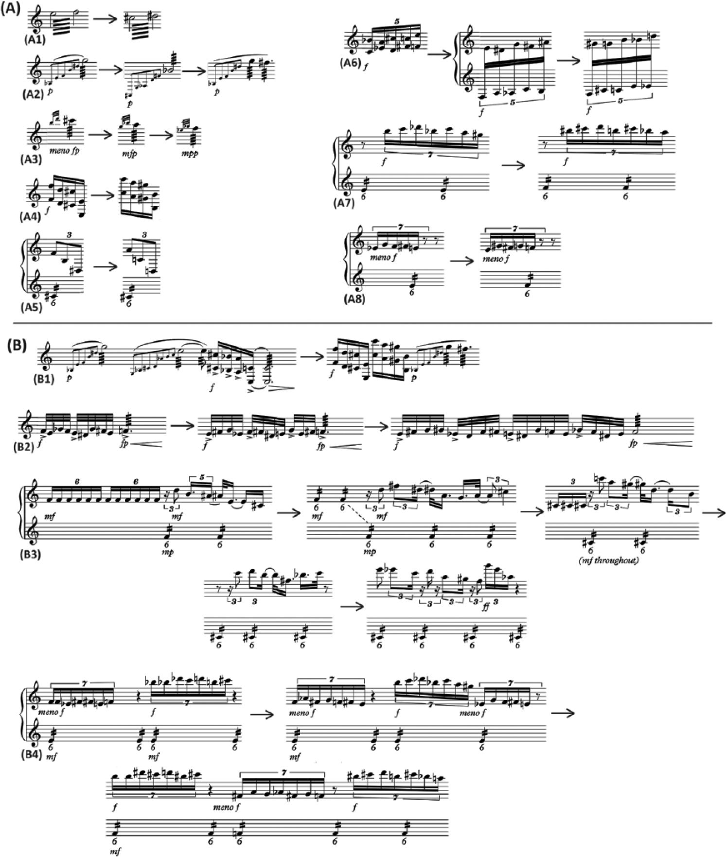
Illustrative musical examples of different cells (panel A) and phrases (panel B), and their repetitions.

A cell or phrase of musical material that is similar to a previous cell or phrase received an incrementally higher score than a cell or phrase of new musical material. The system for scoring musical repetition of cells and phrases is outlined in Table 1. Cells of music rests notated in the score, and presenting as silence in the performance, were scored as 0.5. Figure 3 provides examples of cell and phrase repetition scoring.

Table 1.

Scoring musical repetition of cells and phrases.

Scoring cells/phrases	Scoring the degree of repetition for elements in the system	Score	Final repetition score used in the analysis
Cell*	New/first presentation	1
	Repeat with modifications	2
	Exact repeat	3
	Second repeat with modifications	4
	Second exact repeat	5
	…	…
			Cell, pitch material and rhythmic elements are scored separately, then summed for a final cell repetition score
Phrase**	First presentation	1
	First repeat	2
	Second repetition	3
	…	…
	Fifth repetition	6
			The phrase repetition score is the final score (i.e. there are no separate summed components)

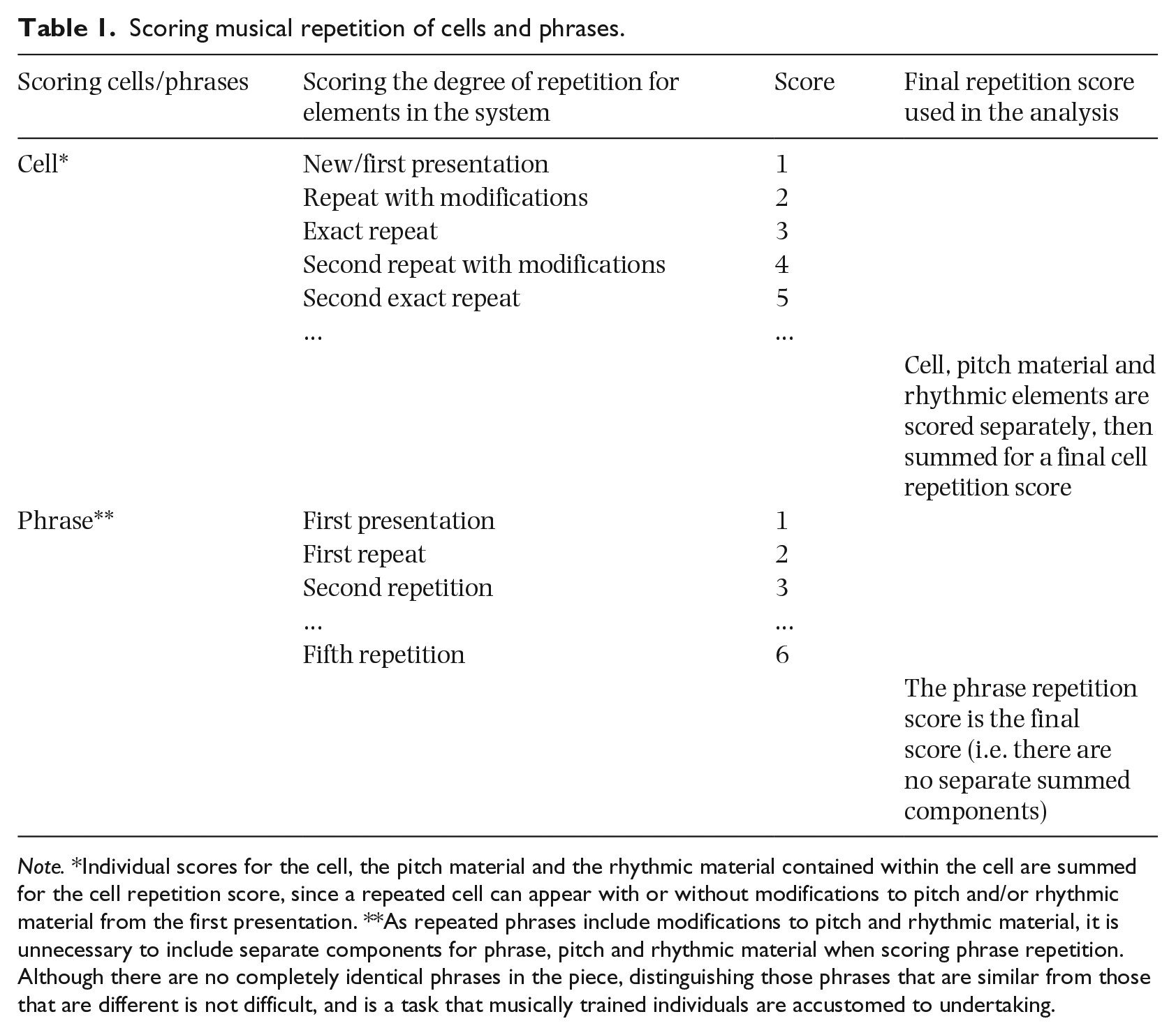
Note. *Individual scores for the cell, the pitch material and the rhythmic material contained within the cell are summed for the cell repetition score, since a repeated cell can appear with or without modifications to pitch and/or rhythmic material from the first presentation. **As repeated phrases include modifications to pitch and rhythmic material, it is unnecessary to include separate components for phrase, pitch and rhythmic material when scoring phrase repetition. Although there are no completely identical phrases in the piece, distinguishing those phrases that are similar from those that are different is not difficult, and is a task that musically trained individuals are accustomed to undertaking.

Figure 3.

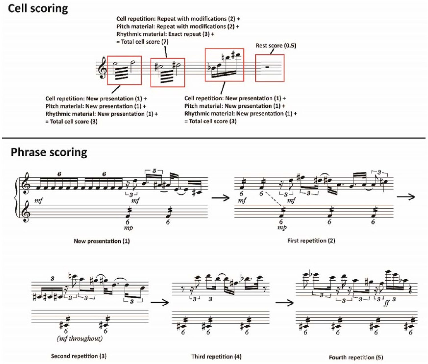
Examples of the scoring of cell and phrase repetition.

Scores for cell and phrase repetition, and notated rests are documented at 500-ms sample intervals on the data file in columns adjacent to the engagement response data. Since these scores usually relate to musical material that is of a longer duration than 500 ms, the score for a cell, phrase or rest endures for each 500-ms sample within the cell/phrase/rest.

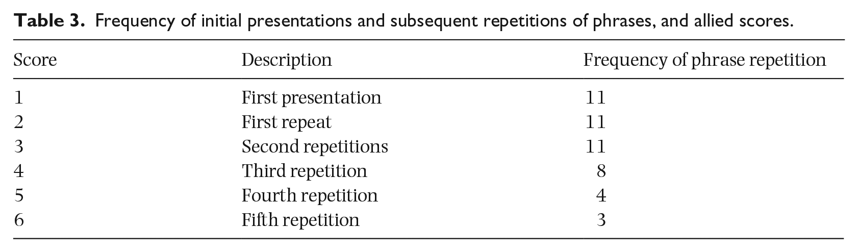
Through the analytical process a total number of 157 cells, 48 phrases, and 11 cells of silence (i.e., rests) were identified. The mean duration of cells was 1.68 s (SD = 1.7 s), 5.35 s (SD = 4.43 s) for phrases, and 2.4 s (SD = 1.68 s) for rests. In relation to the structure of the piece, Section A contained 22 cells (mean duration = 3 s, SD = 2.82 s), 7 phrases (mean duration = 9.43 s, SD = 8.44 s), and 2 rests (mean duration = 3.25 s, SD = 0.35 s). Section B contained 100 cells (mean duration = 10.1 s, SD = 0.48 s), 27 phrases (mean duration = 3.74 s, SD = 1.20 s), and 1 rest (duration = 6.5 s). Section A2/Coda contained 34 cells (mean duration = 2.79 s, SD = 1.99 s), 14 phrases (mean duration = 6.43 s, SD = 4.42 s), and 7 rests (mean duration = 1.57 s, SD = 0.61 s). Table 2 shows the overall frequency of initial presentation and subsequent repetitions of cells, and allied scores. Also noted in Table 2 are the overall frequencies of initial presentations and subsequent repetitions of pitch and rhythmic elements in cells and scoring. Table 3 shows the overall frequency of initial presentation and subsequent repetitions of phrases, and allied scores.

Table 2.

Frequency of initial presentation and repetitions of cells, the pitch and rhythmic material contained in cells, and allied scores.

		Frequency of repetition
Score	Description	Cell	Pitch material	Rhythmic material
1	New/first presentation	54	54	52
2	Repeat with modifications	42	39	3
3	Exact repeat	15	17	45
4	Second repeat with modifications	16	17
5	Second exact repeat	4	4	16
6	Third repeat with modifications	8	8
7	Third exact repeat	3	3	10
8	Fourth repeat with modifications	3	3
9	Fourth exact repeat	2	2	5
10	Fifth repeat with modifications	2	2
11	Fifth exact repeat	2	2	5
12	Sixth repeat with modifications	3	3
13	Sixth exact repeat			3
14	Seventh repeat with modifications	3	3
15	Seventh exact repeat			5
17	Eighth exact repeat			2
19	Ninth exact repeat			1
21	Tenth exact repeat			2
23	Eleventh exact repeat			1
25	Twelfth exact repeat			1
27	Thirteenth exact repeat			2
29	Fourteenth exact repeat			1
31	Fifteenth exact repeat			1
33	Sixteenth exact repeat			1
35	Seventeenth exact repeat			1

Table 3.

Frequency of initial presentations and subsequent repetitions of phrases, and allied scores.

Score	Description	Frequency of phrase repetition
1	First presentation	11
2	First repeat	11
3	Second repetitions	11
4	Third repetition	8
5	Fourth repetition	4
6	Fifth repetition	3

Density scores were determined through visual inspection of the .wav file spectrum display for note onsets during each 500-ms sample and the music score, and listening to the performance recording. Note onsets were easily visually identifiable in the spectrum display due to the quick decay time characteristic of the struck marimba (Fletcher & Rossing, 1998). To create the illusion of a sustained sound, the marimbist performs a roll technique, in which they strike the marimba bar(s) with alternating hands in quick succession. In the present study, only the first strike of the roll was treated as the onset of the event. The frequency of discrete note onsets in each 500-ms sample was summed for a note density score per sample. In other words, the units of note density were based on the number of distinct onsets per sample. The note density scores (hence “Density”) were documented on the data file in a column adjacent to the engagement response data at each related 500-ms sample. A mean note density score of 2.08 (SD = 1.71) per sample was recorded. In relation to the structure of the piece, Section A had a mean density score of 1.29 (SD = 1.01), Section B had a mean note density score of 3.52 (SD = 1.70), and Section A2/Coda had a mean note density score of 1.2 (SD = 0.98).

Sound intensity was extracted from the audio signal, and processed via PRAAT (Boersma & Weenink, 2005). The “IntensityTier” object was used to generate the time series of the intensity levels, which were then exported for further analysis. The physical sound intensity values (hence “Intensity”) were aligned with participants’ continuous self-report engagement response data at the 500-ms sample to which they pertained for statistical analyses.

Data preparation

Sample-by-sample mean engagement scores were calculated to produce a mean engagement time series. All four exogenous variables were smoothed using the method proposed by Velleman and Hoaglin (1981) as implemented in the SPSS T4253H (SPSS, 2006, pp. 108–109) routine. All variables were transformed into z-scores for ease of comparison. Figure 4 shows a time series plot of the mean engagement (hence “Engagement”) time series with the exogenous variables superimposed.

Figure 4.

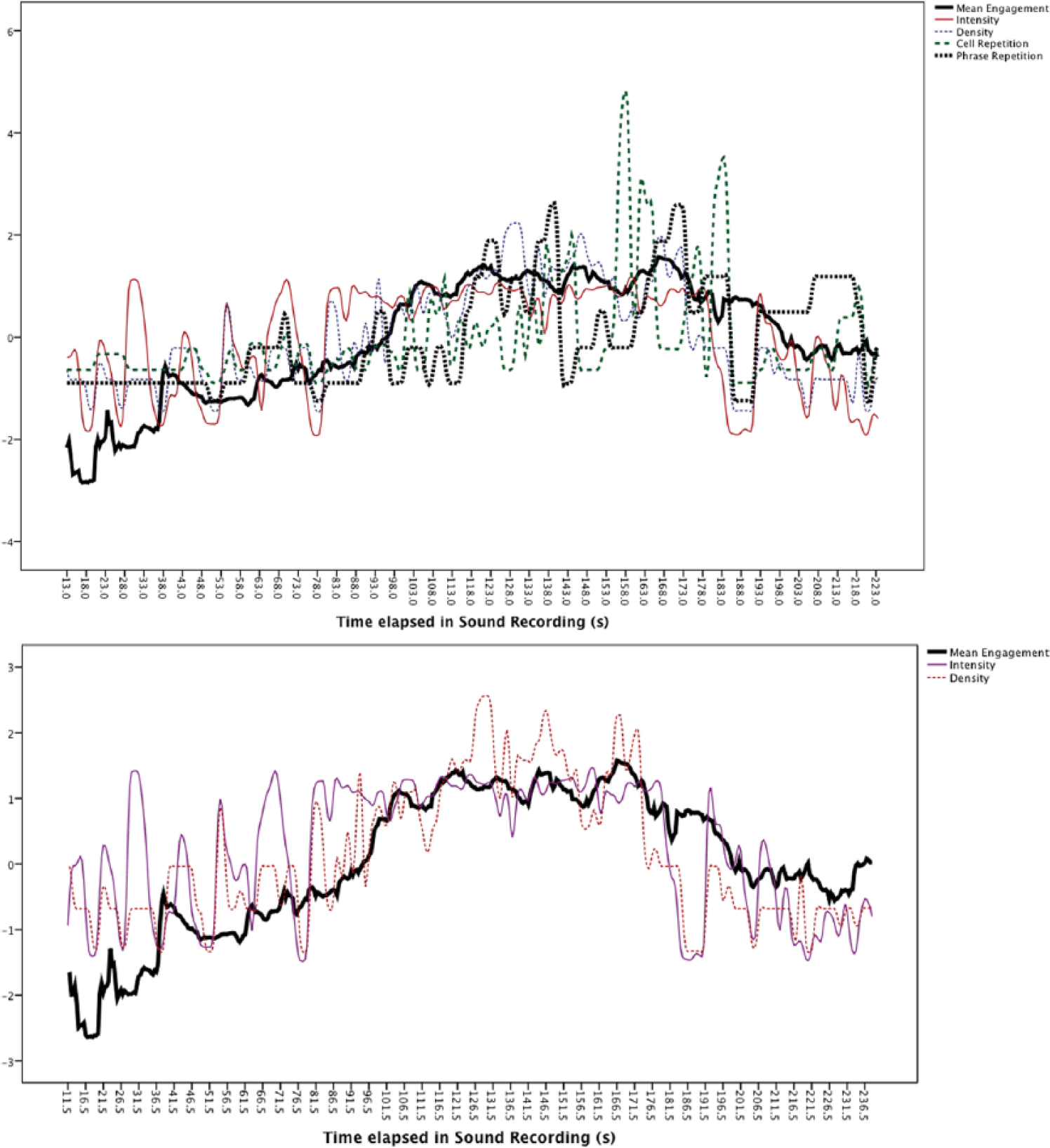
Time series of smoothed z-score variables. Top panel, mean Engagement, with all four exogenous variables. Bottom panel, mean Engagement, with Intensity and Density (for greater clarity).

Initial analysis by visual inspection

Visual inspection of the figure suggests that while a general build up and release can be observed in the two repetition measures that follow the general trajectory of Engagement, there are also several points when the opposite is observed. Note for example in the range t = 140–150 s for both repetition variables compared to Engagement (see Figure 5). Of the four exogenous (“predictor”) variables, Intensity and Density “follow” the pattern of Engagement more closely in the time series plot than do the two repetition measures.

Figure 5.

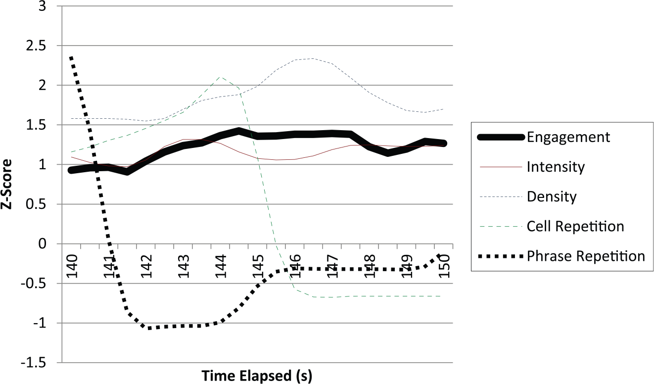
Mean Engagement and four exogenous variables over the period t = 140 - 150 s. The period presents an example of contradictory movements in cell and phrase repetition with respect to mean Engagement.

Quantitative analysis employed the Box–Jenkins (Box, Jenkins, & Reinsel, 1994) ARIMA (Autoregressive Integrated Moving Average) transfer function procedure, which processes multivariate exogenous variables while dealing with serial correlation. The analytic approach used to investigate time series analysis is described in the online supplementary file, “Development of, and rationale for the time-series analysis applied to Broughton et al.”.

Results

The following observations are made about the analysis. Sampling periods of 1 and 2 produced complex ARIMA models (MA parameter of 16 or greater) as predicted, and so were omitted from further analysis. From sampling period of 3 onward, ARIMA model parameters became stable and parsimonious with 91.08% of the remaining 1,278 procedures identifying a (0, 1, 0) process, indicating that a first order integrative process (hence the “1” as the order of the I parameter in the middle of the triad) regularly produced a valid model. This model is easily interpretable because it can be thought of as modelling changes in engagement rating (Schubert, 2002). Of particular interest in the analysis is which, if any, of the exogenous variables were included. Density was reported most frequently (in 228 models), followed by Intensity (177 models), then cell repetition (18) and phrase repetition (8). The SPSS Expert Modeler (EM) procedure eliminated variables that did not make a significant contribution to the variance. However, the procedure did not guarantee an optimal model at each sampling period, and so a statistical analysis of the residual for each of these models was further investigated.

The Ljung–Box test (Ljung & Box, 1978) estimates the likelihood that the residual of the model is random noise by examining the autocorrelations at different lags of the model residual. This approach allows the diagnosis of the presence of serial correlation (or perhaps more appropriately, the absence of serial correlation if the test returns non-significant results). We inspected the p-value for the Ljung–Box statistic for each “sampling period by offset” procedure, and did indeed observe some reported models where serial correlation was found in the residual. The plot of the p-value for the Ljung–Box output for each model is shown in Figure 6. To reduce the number of incorrectly identified serially correlated residuals due to chance, the results were inspected with respect to a more liberal significance threshold of p = .2, compared to the more common p = .05. In this way we can see a range of sampling periods, 11 to 16, with more-or-less uninterrupted serial-correlation-free models (higher than the recommended sampling range of 9). Furthermore, as the sampling period approaches 21 we start to see an increasing prevalence of significant residuals (p < .05) until sampling period 23 when the models cease to produce valid or calculable residual analysis statistics. We interpreted this to mean that the models in the range of sampling period 11 to 16 were overall valid, and this informed our interpretation of the exogenous variable that made a “true” contribution to Engagement ratings.

Figure 6.

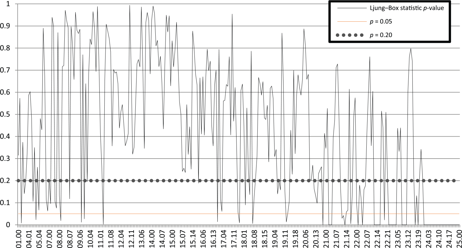
Ljung–Box statistic significance readings across the range of sampling periods and offsets (the first two digits on the x-axis are sampling period, the last two are offset within sampling period). Note that the sampling periods 11 to 16 produced models with generally large p-values, meaning that those models had little probability of containing serial correlation in their residuals.

To further explain, consider the significant variables reported by each EM procedure, as summarised in Figure 7. The figure shows the prevalence of each exogenous variable in the EM procedures. That is, for each sampling period, there was one model generated for each offset, and it is the sums of the count of significant variable coefficients for each exogenous variable that are shown in the figure. However, since there will be progressively more models as the sampling period increases (e.g., the sampling period of 30 generates 30 models, from offset 0 to offset 29), the tally of significant variables is divided by the number of offsets for each sampling period. Hence the figure reports the proportion of variables represented by the models at each sampling period, allowing comparison across sampling periods. The figure indicates that two exogenous variables are dominant: Density is represented fairly consistently from sampling period 10 onwards, while Intensity dominates over the first 10 sampling periods, disappears, and then returns at sampling period 17.

Figure 7.

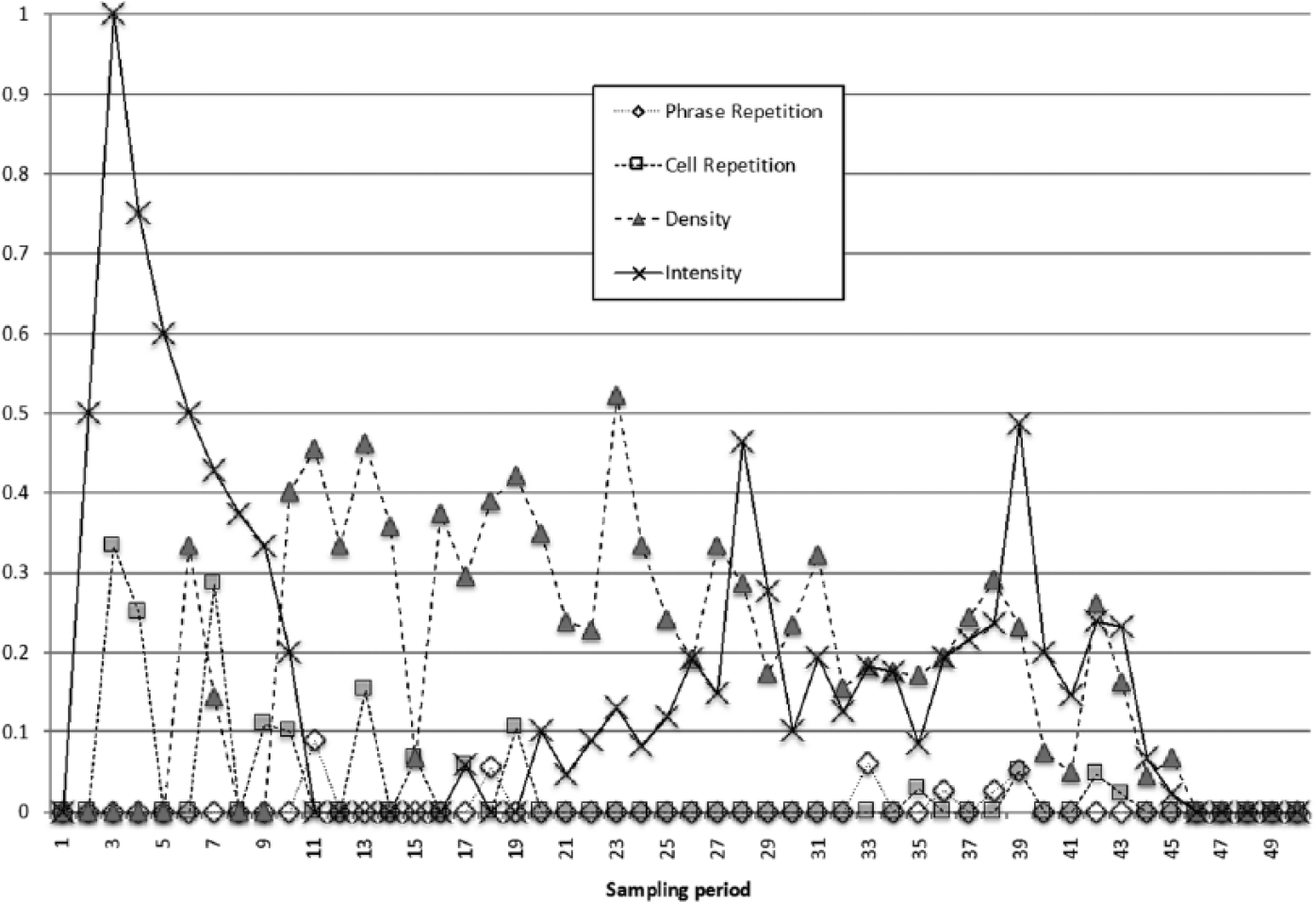
Proportion of statistically significant exogenous variable coefficients as a ratio of total number of offset models per sampling period. Note the prevalence of Intensity and Density at different sampling periods, compared to the relative scarcity of the repetition variables in presenting significant predictors of Engagement. This demonstrates that the latter two made little contribution to the Autoregressive Integrated Moving Average (ARIMA) transfer models.

This particular pattern provides a critical clue that allows us to make a stronger conclusion than might have been possible if using only one, fixed, small sampling period, because the dominance of Density as an explanatory variable coincides when the models produced have residuals that are statistically identical to random noise. That is, both the quantity of Density variable selections and the quality of the models in which the Density variable appears encourage us to conclude that Density contributes significantly and fairly independently to changes in Engagement ratings. Intensity, on the other hand, while making a significant contribution to the models at several sampling periods, tended to be significant when there was relatively more serial correlation in the models (the Ljung–Box statistic was occasionally significant).

Discussion

The present study investigated relationships between musical repetition, Density and Intensity, and observers’ continuous self-report responses of Engagement with an unfamiliar, atonal post-serialist solo marimba work performed live. As expected, Density and Intensity contributed to observer Engagement with the performance. However, contrary to our expectations, the repetition variables did not contribute so strongly to observer Engagement.

In the present study, the repetition of musical motives and phrases in the single, live performance appears not to have been recognised. This is contrary to experimental evidence suggesting that under certain conditions listeners can learn an artificial grammar from which unfamiliar music can be constructed (Loui et al., 2010), and detect musical similarity between adjacent and non-adjacent segments of music (Creel et al., 2004) within an experimental session (Rohrmeier et al., 2011). Considering motivic cells and phrases as being the music’s microstructure, a certain threshold of repeated exposure (Stevens et al., 2013) might be especially important for developing implicit knowledge for the structure of non-diatonic music. The musical microstructure investigated might have been overly complex for observers to develop structural knowledge in just one pass. The present study results show little evidence that observers recognise repeating musical motives and phrases (cf. Egermann et al., 2013; McAdams et al., 2004) in live music performance, where the music is constructed from an unfamiliar, non-diatonic base. Repeating the entire performance might have had a positive effect on observers’ developing understanding of the musical microstructure, and enabled observers to attend to different facets of the music on successive exposures (Margulis, 2012). Repeated exposure would likely support observers in developing long-term memory and working memory strategies to deal with the musical material encountered (McAdams et al., 2004; Zajonc, 1968, 2001).

It is possible that the musically trained and untrained observers here responded differently to musical repetition. Musical repetition, be it immediate or delayed, plays an important role in non-expert listeners’ aesthetic responses to atonal music (Margulis, 2013). Yet, when experienced listeners are faced with serial (atonal) music, they base their understanding of the music’s grammatical structure on the lack of repetition and avoidance of a sense of tonality associated with pitch relations – the “antistructure” (Ockelford & Sergeant, 2013). As the majority of observers in the present study were musically trained, it is possible that musical repetition made less of a contribution to these observers’ developing understanding of the music structure of the piece than to that of musically untrained observers. Furthermore, as the majority of observers were musically trained, it is possible that their responses dominated mean Engagement ratings.

The method used to analyse and score musical repetition in the present study could be refined. The idea of creating measures of musical repetition from a motivic cell level is supported empirically (Egermann et al., 2013). Thorpe, Ockelford, and Aksentijevic (2011) provide some empirical support for the Zygonic model, and its bases of repetition in the music structure and expectation, with tonal music. However, observers are possibly less sensitive to the underlying structure when the music is assembled from a relatively unfamiliar atonal (Dibben, 1994), compared to a more familiar tonal base (Krumhansl, 1996; Livingstone et al., 2012).

Lacking a familiar tonal structure and possibly insufficient exposure to form a reliable understanding of the music’s motivic cell and phrase structure, Density emerged as the primary contributor to observers’ Engagement with the music performance. Interestingly, results indicated a relationship between the macro structure of the piece and Density. Specifically, the section of the music that featured the highest density of notes was the middle section of the piece, Section B, which contrasted with the musically similar Sections A and A2/Coda surrounding it. High note Density was the musical feature that appeared to provide observers with a solid foundation in unfamiliar musical territory from which to effectively segment the musical surface, embark on categorical processes and develop a mental representation of the music structure at some level (Deliège, 1996, 2001, 2007; Deliège et al., 1996). If repetition had been important to observers’ Engagement with the performance at the macro level of the music structure, then one would have expected the final A2/Coda section to have attracted higher responses from observers than Section A or the highly note-dense Section B. This was not observed, strengthening our conclusion that Density makes a stronger contribution to observer Engagement with unfamiliar music performed live than musical repetition.

Our findings for Density appear to support the notion that the temporal facet of music makes a fundamental contribution to observer Engagement with performance. The Density results resemble those of previous research identifying positive relationships between tempo and affective responses (Balch & Lewis, 1996; Dalla Bella et al., 2001; Gagnon & Peretz, 2003; Husain et al., 2002; Webster & Weir, 2005). Although the musical stimuli performed in the present study did not have an obvious beat or metrical structure, increasing note Density might have provided more regularity in the periodicity of events, enabling observers to infer a sense of beat, and thus develop temporal expectations. Dynamic Attending Theory posits that the mechanism underpinning listener attentional behaviour is entrainment of internal oscillations to external stimuli, which drives expectations (Large & Jones, 1999). Empirical evidence supports this notion through demonstrating that observers’ neural activity, or oscillations, entrain to the perceived beat and meter induced through audio-only, or synchronous audio-visual rhythmic stimuli (Nozaradan, 2014). This has also been demonstrated through listeners’ neural responses to ecologically valid music (Tierney & Kraus, 2015). Of course, the results we observed could be specific to the music performed for this study. Replication with more and varied types of music would strengthen our findings, as would systematic investigation through an experimental approach.

As the concept of Engagement with the social and physical environment is proposed to incorporate perceptual, cognitive and affective elements (Furrer & Skinner, 2003; Reeve et al., 2004; Russell et al., 2005), it is plausible that observers’ Engagement responses to the synchronous audio-visual, live music performance experience reflect the combined outcome of different processes. Increases in Density often correspond to increases in the amount of physical movement in marimba playing, and thus, visual information, generated. Previous research shows that increased physical movement that is allied to the production of a musical performance might indicate greater levels of expression to observers (Antonietti, Cocomazzi, & Iannello, 2009; Broughton & Stevens, 2009; Davidson, 1993, 1994; Huang & Krumhansl, 2011; Juchniewicz, 2008); reducing movement can result in diminished performance- and performer-related judgments (Nusseck & Wanderley, 2009). Therefore, the visual as well as auditory information generated in sections of high note density might have been more interesting (Broughton & Stevens, 2009) to observers, contributing to enjoyment and situational interest (Chen, Darst, & Pangrazi, 2001) in the task, and heightening engagement with, and enjoyment of (Thompson, 2007) the performance material. This suggests that observers’ Engagement responses might be more closely linked to “bottom-up” processing of auditory, and perhaps visual, sensory information, than cognitive processing associated with musical repetition. This idea receives some support from previous experimental research reporting that listener engagement mediates the relationship between the physical properties of musical sound and listeners’ affective responses (Olsen et al., 2014).

Intensity might be a strong contributor to several aesthetic/affective responses to music (Bailes & Dean, 2012; Dean et al., 2011; Schubert, 2004), but the present results suggest that Density also plays an important role. We were able to generate models that could identify a fairly independent role for Density in predicting Engagement responses, which we found more difficult to do for Intensity. This might indicate that music does not need to be loud, if it is dense, to be engaging.

Serial correlation was initially the dominant variable, necessitating statistical control in order to examine the contribution of other variables of interest. For the change in response of Engagement with a contemporary marimba piece performed live, serial correlation propagates through the system over a period of about 5 s, after which time the influence of exogenous variables acts fairly independently upon the change in ratings. We presented an alternative method for analysis, which considered the benefits of examining multiple models at a range of sampling periods as an additional way of managing serial correlation in the system of interest.

The results indicate that Density may be an important musical feature for observers of unfamiliar live music performance with which to engage. However, the findings should be considered in light of the study limitations. Conducting research within a live performance context provides a degree of authenticity to the nature of music performance and observer response. However, stringent experimental control is necessarily sacrificed for this authenticity. We cannot discount the potential effects that uncontrolled variables, such as visual information, and even the venue, lighting and seating arrangements might have had on observers’ Engagement with the live performance. The present findings do suggest interesting pathways for future research, incorporating experimental approaches, to better understand how observers engage with unfamiliar musical works.

Conclusions

Results of our study using a new modelling approach show that note Density, and to a lesser degree, Intensity, make a noticeable contribution to observers’ Engagement with unfamiliar music performed live. Repetition variables appear to make less of a contribution to Engagement responses in this context. A single performance seems to provide observers with insufficient exposure to comprehend and respond to the structure of atonal music. On the other hand, Density appears to facilitate observers to segment the musical surface and develop an understanding of the music structure at some level. Increasing note Density potentially drives Engagement with unfamiliar music performed live through stimulus-driven entrainment processes shaping attentional behaviour and musical expectations. As any percussionist will attest – the temporal facet of live music performance appears to be fundamental to observer Engagement. Studies in live performance contexts are crucial to developing understanding of how observers experience and respond to artistic performance practices. Through understanding how observers respond to, and interact with artistic performance (see Burland & Pitts, 2014), we are better placed to develop audiences for unfamiliar music performance practices, and create and present live music to optimal effect.

Footnotes

Authors’ Note

The development of, and rationale for the time-series analysis approach applied in the article is available online as a supplementary file.

Ethical considerations

Ethical approval for this project was given by Western Sydney University Human Research Ethics Committee [ref number HREC 04/087]. Data can be obtained by emailing the corresponding author.

Funding

The authors received no financial support for the research, authorship, and/or publication of this article.

References

Antonietti

Cocomazzi

Iannello

(2009). Looking at the audience improves music appreciation. Journal of Nonverbal Behavior, 33, 89–106. doi:10.1007/s10919–008–0062-x

Bailes

Dean

R. T.

(2012). Comparative time series analysis of perceptual responses to electroacoustic music. Music Perception, 29, 359–375. doi:10.1525/mp.2012.29.4.359

Balch

W. R.

Lewis

B. S.

(1996). Music-dependent memory: The roles of tempo changes and mood mediation. Journal of Experimental Psychology: Learning, Memory and Cognition, 22, 1354–1363. doi:10.1037/0278–7393.22.6.1354

Bharucha

J. J.

Krumhansl

C. L.

(1983). The representation of harmonic structure in music: Hierarchies of stability as a function of context. Cognition, 13, 63–102. doi:10.1016/0010–0277(83)90003–3

Bigand

(1993). The influence of implicit harmony, rhythm and musical training on the abstraction of “tension-relaxation schemas” in tonal musical phrases. Contemporary Music Review, 9, 123–137. doi:10.1080/07494469300640391

Bigand

Poulin-Charronnat

(2006). Are we “experienced listeners”? A review of the musical capacities that do not depend on formal musical training. Cognition, 100, 100–130. doi:10.1016/j.cognition.2005.11.007

Boersma

Weenink

(2005). PRAAT: Doing phonetics by computer [Computer program]. Version, 5, 21.

Box

G. E. P.

Jenkins

G. M.

Reinsel

G. C.

(1994). Time series analysis: Forecasting and control (3rd ed.). New Jersey: Prentice-Hall.

Broughton

Stevens

(2009). Music, movement and marimba: An investigation of the role of movement and gesture in communicating musical expression to an audience. Psychology of Music, 37, 137–153. doi:10.1177/0305735608094511

10.

Broughton

Stevens

Schubert

(2008). Continuous self-report of engagement to live solo marimba performance. In Miyazaki

Hiraga

Adachi

Nakajima

Tsuzaki

(Eds.), Tenth international conference on music perception and cognition (pp. 366–371). Sapporo, Japan.

11.

Burland

Pitts

(2014). Postlude. In Burland

Pitts

(Eds.), Coughing and clapping: Investigating audience experience (pp. 175–179). Aldershot, UK: Ashgate.

12.

Cambouropoulos

(2009). How similar is similar? Musicae Scientiae, 13(1 suppl), 7–24. doi:10.1177/102986490901300102

13.

Chen

Darst

P. W.

Pangrazi

R. P.

(2001). An examination of situational interest and its sources. British Journal of Educational Psychology, 71, 383–400. doi:10.1348/000709901158578

14.

Cone

E. T.

(1987). On derivation: Syntax and rhetoric. Music Analysis, 6, 237–255. doi:10.2307/854204

15.

Creel

S. C.

Newport

E. L.

Aslin

R. N.

(2004). Distant melodies: Statistical learning of nonadjacent dependencies in tone sequences. Journal of Experimental Psychology: Learning, Memory, and Cognition, 30, 1119–1130. doi:10.1037/0278–7393.30.5.1119

16.

Dalla Bella

Peretz

Rousseau

Gosselin

. (2001). A developmental study of the affective value of tempo and mode in music. Cognition, 80, B1–10. doi:10.1016/S0010–0277(00)00136–0

17.

Davidson

J. W.

(1993). Visual perception of performance manner in the movements of solo musicians. Psychology of Music, 21, 103–113. doi:10.1177/030573569302100201

18.

Davidson

J. W.

(1994). Which areas of a pianist’s body convey information about expressive invention to an audience? Journal of Human Movement Studies, 26, 279–301.

19.

Dean

R. T.

Bailes

Schubert

(2011). Acoustic intensity causes perceived changes in arousal levels in music: An experimental investigation. PLoS ONE, 6(4), e18591. doi:10.1371/journal.pone.0018591

20.

Deliège

(1996). Cue abstraction as a component of categorisation processes in music listening. Psychology of Music, 24, 131–156. doi:10.1177/0305735696242007

21.

Deliège

(2001). Similarity perception ↔ Categorization ↔ Cue abstraction. Music Perception, 18, 233–243. doi:10.1525/mp.2001.18.3.233

22.

Deliège

(2007). Similarity relations in listening to music: How do they come into play? Musicae Scientiae, 11(1 suppl), 9–37. doi:10.1177/1029864907011001021

23.

Deliège

Mélen

Stammers

Cross

(1996). Musical schemata in real-time listening to a piece of music. Music Perception, 14, 117–159. doi:10.2307/40285715

24.

Dibben

(1994). The cognitive reality of hierarchic structure in tonal and atonal music. Music Perception, 12, 1–25. doi:10.2307/40285753

25.

Egermann

Pearce

M. T.

Wiggins

G. A.

McAdams

(2013). Probabilistic models of expectation violation predict psychophysiological emotional responses to live concert music. Cognitive, Affective, & Behavioral Neuroscience, 13, 533–553. doi:10.3758/s13415–013–0161-y

26.

Fletcher

N. H.

Rossing

T. D.

(1998). The physics of musical instruments (2nd ed.). New York, NY: Springer Science & Business Media.

27.

Furrer

Skinner

(2003). Sense of relatedness as a factor in children’s academic engagement and performance. Journal of Educational Psychology, 95, 148–162. doi:10.1037/0022–0663.95.1.148

28.

Gagnon

Peretz

(2003). Mode and tempo relative contributions to “happy-sad” judgments in equitone melodies. Cognition and Emotion, 17, 25–40. doi:10.1080/02699930302279

29.

Hanninen

D. A.

(2003). A theory of recontextualization in music: Analyzing phenomenal transformations of repetition. Music Theory Spectrum, 25, 59–97. doi:10.1525/mts.2003.25.1.59

30.

Huang

Krumhansl

C. L.

(2011). What does seeing the performer add? It depends on musical style, amount of stage behavior, and audience expertise. Musicae Scientiae, 15, 343–364. doi:10.1177/1029864911414172

31.

Husain

Thompson

W. F.

Schellenberg

E. G.

(2002). Effects of musical tempo and mode on arousal, mood, and spatial abilities. Music Perception, 20, 151–171. doi:10.1525/mp.2002.20.2.151

32.

Ichiyanagi

(1991). The source for solo marimba [music composition]. Tokyo, Japan: Schott.

33.

Juchniewicz

(2008). The influence of physical movement on the perception of musical performance. Psychology of Music, 36, 417–427. doi:10.1177/0305735607086046

34.

Kivy

(1993). The fine art of repetition: Essays in the philosophy of music. Cambridge, UK: Cambridge University Press.

35.

Krumhansl

C. L.

(1996). A perceptual analysis of Mozart’s Piano Sonata K. 282: Segmentation, tension, and musical ideas. Music Perception, 13, 401–432. doi:10.2307/40286177

36.

Krumhansl

C. L.

Kessler

E. J.

(1982). Tracing the dynamic changes in perceived tonal organization in a spatial representation of musical keys. Psychological Review, 89, 334–368. doi:10.1037/0033–295x.89.4.334

37.

Large

E. W.

Jones

M. R.

(1999). The dynamics of attending: How people track time-varying events. Psychological Review, 106, 119–159. doi:10.1037/0033–295X.106.1.119

38.

Lerdahl

Jackendoff

(1983). A generative theory of tonal music. Cambridge, MA: MIT Press.

39.

Livingstone

S. R.

Palmer

Schubert

(2012). Emotional response to musical repetition. Emotion, 12, 552–567. doi:10.1037/a0023747

40.

Ljung

G. M.

Box

G. E. P.

(1978). On a measure of lack of fit in time series models. Biometrika, 65, 297–303. doi:10.1093/biomet/65.2.297

41.

Loui

Wessel

D. L.

Hudson Kam

C. L.

(2010). Humans rapidly learn grammatical structure in a new musical scale. Music Perception, 27, 377–388. doi:10.1525/mp.2010.27.5.377

42.

Lucas

B. J.

Schubert

Halpern

A. R.

(2010). Perception of emotion in sounded and imagined music. Music Perception, 27, 399–412. doi:10.1525/mp.2010.27.5.399

43.

Margulis

E. H.

(2012). Musical repetition detection across multiple exposures. Music Perception, 29, 377–385. doi:10.1525/mp.2012.29.4.377

44.

Margulis

E. H.

(2013). Aesthetic responses to repetition in unfamiliar music. Empirical Studies of the Arts, 31, 45–57. doi:10.2190/EM.31.1.c

45.

Margulis

E. H.

(2014). On repeat: How music plays the mind. New York, NY: Oxford University Press.

46.

McAdams

Vines

B. W.

Vieillard

Smith

B. K.

Reynolds

(2004). Influences of large-scale form on continuous ratings in response to a contemporary piece in a live concert setting. Music Perception, 22, 297–350. doi:10.1525/mp.2004.22.2.297

47.

Nozaradan

(2014). Exploring how musical rhythm entrains brain activity with electroencephalogram frequency-tagging. Philosophical Transactions of the Royal Society B, 369, 20130393. doi:10.1098/rstb.2013.0393

48.

Nusseck

Wanderley

M. M.

(2009). Music and motion: How music-related ancillary body movements contribute to the experience of music. Music Perception, 26, 335–353. doi:10.1525/mp.2009.26.4.335

49.

Ockelford

(2005). Repetition in music: Theoretical and metatheoretical perspectives. Aldershot, UK: Ashgate.

50.

Ockelford

(2009). Similarity relations between groups of notes: Music-theoretical and music-psychological perspectives. Musicae Scientiae, 13, 47–98. doi:10.1177/102986490901300104

51.

Ockelford

Sergeant

(2013). Musical expectancy in atonal contexts: Musicians’ perception of “antistructure”. Psychology of Music, 41, 139–174. doi:10.1177/0305735612442582

52.

Olsen

K. N.

Dean

R. T.

Stevens

C. J.

(2014). A continuous measure of musical engagement contributes to prediction of perceived arousal and valence. Psychomusicology, 24, 147–156. doi:10.1037/pmu0000044

53.

Poulin-Charronnat

Bigand

Lalitte

Madurell

Vieillard

McAdams

(2004). Effects of a change in instrumentation on the recognition of musical materials. Music Perception, 22, 239–263. doi:10.1525/mp.2004.22.2.239

54.

Reeve

Jang

Carrell

Jeon

Barch

(2004). Enhancing students’ engagement by increasing teachers’ autonomy support. Motivation and Emotion, 28, 147–169. doi:10.1023/B:MOEM.0000032312.95499.6f

55.

Reynolds

(2004). Compositional strategies in The Angel of Death for piano, chamber orchestra and computer-processed sound. Music Perception, 22, 173–205. doi:10.1525/mp.2004.22.2.173

56.

Rohrmeier

Rebuschat

Cross

(2011). Incidental and online learning of melodic structure. Consciousness and Cognition, 20, 214–222. doi:10.1016/j.concog.2010.07.004

57.

Russell

V. J.

Ainley

Frydenberg

(2005). Schooling issues digest: Student motivation and engagement. Retrieved from http://www.dest.gov.au/sectors/school_education/publications_resources/schooling_issues_digest/schooling_issues_digest_motivation_engagement.htm

58.

Schubert

(2002). Correlation analysis of continuous emotional response to music: Correcting for the effects of serial correlation. Musicae Scientiae, 5, 213–236. doi:10.1177/10298649020050s108

59.

Schubert

(2004). Modelling perceived emotion with continuous musical features. Music Perception, 21, 561–585. doi:10.1525/mp.2004.21.4.561

60.

Schubert

Vincs

Stevens

C. J.

(2013). Identifying regions of good agreement among responders in engagement with a piece of live dance. Empirical Studies of the Arts, 31, 1–20. doi:10.2190/EM.31.1.a

61.

SPSS. (2006). SPSS 15.0 Algorithms. Chicago, IL: SPSS Inc.

62.

Stevens

C. J.

Schubert

Haszard Morris

R. H.

Frear

Chen

Healey

… Hansen

(2009). Cognition and the temporal arts: Investigating audience response to dance using PDAs that record continuous data during live performance. International Journal of Human-Computer Studies, 67, 800–813. doi:10.1016/j.ijhcs.2009.06.001

63.

Stevens

C. J.

Tardieu

Dunbar-Hall

Best

C. T.

Tillmann

(2013). Expectations in culturally unfamiliar music: Influences of proximal and distal cues and timbral characteristics. Frontiers in Psychology, 4. doi:10.3389/fpsyg.2013.00789

64.

Stevens

Vincs

Schubert

(2009). Measuring audience response on-line: An evaluation of the portable Audience Response Facility (pARF). In Stevens

Schubert

Kruithof

Buckley

Fazio

(Eds.), Proceedings of the 2nd International Conference on Music Communication Science (ICoMCS2), published by HCSNet, Western Sydney University.

65.

Thompson

(2007). Determinants of listeners’ enjoyment of a performance. Psychology of Music, 35, 20–36. doi:10.1177/0305735607068886

66.

Thorpe

Ockelford

Aksentijevic

(2012). An empirical exploration of the zygonic model of expectation in music. Psychology of Music, 40, 429–470. doi:10.1177/0305735610392103

67.

Tierney

Kraus

(2015). Neural entrainment to the rhythmic structure of music. Journal of Cognitive Neuroscience, 27, 400–408. doi:10.1162/jocn_a_00704

68.

Velleman

P. F.

Hoaglin

D. C.

(1981). Applications, basics, and computing of exploratory data analysis. Boston, MA: Duxbury Press.

69.

Webster

G. D.

Weir

C. G.

(2005). Emotional responses to music: Interactive effects of mode, texture, and tempo. Motivation and Emotion, 29, 19–39. doi:10.1007/s11031–005–4414–0

70.

Zajonc

R. B.

(1968). Attitudinal effects of mere exposures. Journal of Personality and Social Psychology, 9(2, Pt. 2), 1–27. doi:10.1037/h0025848

71.

Zajonc

R. B.

(2001). Mere exposure: A gateway to the subliminal. Current Directions in Psychological Science, 10, 224–228. doi:10.1111/1467–8721.00154

Supplementary Material

Please find the following supplemental material available below.

For Open Access articles published under a Creative Commons License, all supplemental material carries the same license as the article it is associated with.

For non-Open Access articles published, all supplemental material carries a non-exclusive license, and permission requests for re-use of supplemental material or any part of supplemental material shall be sent directly to the copyright owner as specified in the copyright notice associated with the article.

0.00 MB

0.64 MB