Mass moments of inertia for axisymmetric shells evaluated using the Monte-Carlo method

Abstract

The mass moment of inertia (MMoI) of a truncated conical shell is derived. The MMoI of a truncated conical shell, can be used to model the MMoI for other shapes; a conical shell, a tube, a disc and an annulus. Using the additive property of MMoI, the MMoI for a spherical shell, and a hemispherical shell can also be calculated.

The MMoI is evaluated using the Monte-Carlo method. Two variants of the Monte-Carlo method are derived, named No PAT method and PAT method, differentiated by whether the parallel axis theorem is combined with the Monte-Carlo method or not. The PAT method tends to be the more efficient algorithm.

This paper provides a partial framework for evaluating the MMoI for any axisymmetric body. It is proposed that the calculation of MMoI, for a truncated conical shell, and truncated cones can be used to develop student project activities. By way of examples of potential student projects, the calculation of the MMoI using the Monte-Carlo methods, for the Saturn V rocket, and an American football are demonstrated.

Keywords

Monte-Carlo method mass moment of inertia parallel axis theorem truncated conical shells

Introduction

The Monte-Carlo method is a stochastic approach, that can be applied to many physical and chemical processes, of interest to mechanical engineering students. At the author's university, the Monte-Carlo method is being introduced into the syllabus of an advanced undergraduate course including radiation heat transfer. Experience in implementing this change in advanced course curriculum, has indicated that students require further support in stochastic methods, before encountering radiation heat transfer. It is proposed to introduce the Monte-Carlo method to evaluate mass moment of inertia (MMoI) in an introductory course in mechanics where rotating systems are analyzed.¹

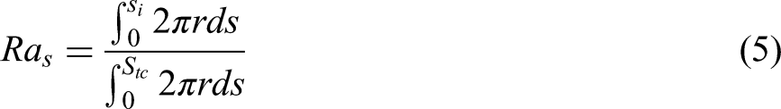
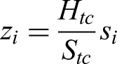
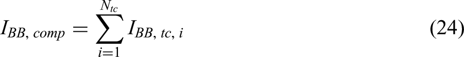
The mass moment of inertia is defined by the integral,

I_{x x} = \int r^{2} d m

(1)

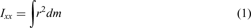
Where r is the perpendicular distance from the axis x-x to a point in the shape. Figure 1 shows parameters defining the MMoI for a general shape. In Figure 1, two axes are shown, labelled as x-x and G-G. The axes are parallel to each other, and the axis G-G intersects the center of mass of the shape. This is important as the parallel axis theorem states,

I_{x x} = I_{G G} + m d^{2}

(2)

Figure 1.

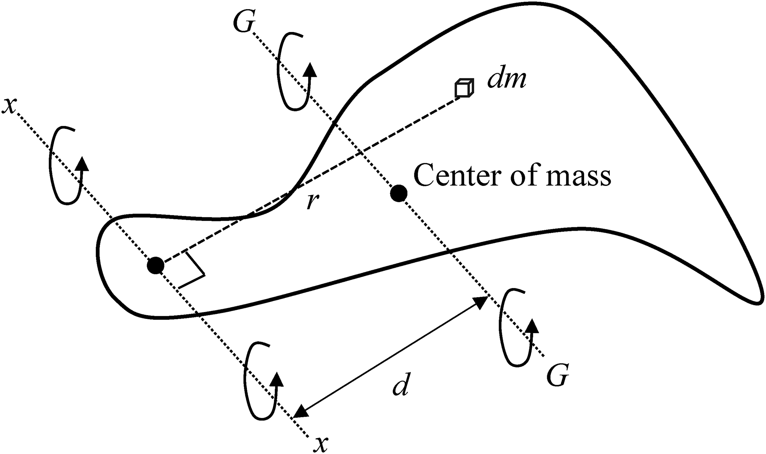
Schematic of a generic shape, the axis of rotation, x-x and the axis G-G through the center of mass.

Where d is the perpendicular distance between the two axes. For 3-dimensional shapes the generalized definition of the MMoI, (1) is a 3-dimensional integral.

In this paper the Monte-Carlo method is used to evaluate the MMoI for a truncated conical shell. This is a companion paper to a paper focused on the evaluation of MMoI of solid truncated cones.² The MMoI for a truncated conical shell in general cannot be found in textbooks on mechanics, and the second more powerful justification for this investigation is that many axisymmetric shell shapes can be represented as limiting cases of truncated conical shells, or as a composite of truncated conical shells. A wide range of axisymmetric shapes can be calculated based on a single Monte-Carlo method implementation. Taking the two papers together it is possible to calculate the MMoI for any composite axisymmetric shape based on a combination of truncated conical shells and truncated cones. This is considered below, with two possible student project-based applications of the analysis, to calculate the MMoI of the Saturn V rocket,³ Appollo 10, and the MMoI of an American football.⁴ The original idea for this paper is the use of the Monte-Carlo method applied to the view factor calculation of axisymmetric systems, where using a truncated cone representation of a range of primitive shapes has many benefits.⁵

The advantages and disadvantages of the Monte-Carlo method compared to deterministic methods are given in² and will be considered only briefly. The Monte-Carlo method can be applied to many multi-dimensional physical and chemical processes.^6–8 To understand the strengths and weaknesses of the Monte-Carlo method, its application to the evaluation of definite integrals will be used to illustrate the Monte-Carlo method basis.^9,10 Consider the numerical quadrature of the 1-dimensional integral,

I = \int_{a}^{b} f (x) d x

(3)

Extending the Monte-Carlo method to multi-dimensional integrals is straight forward. The Monte-Carlo method uses pseudo-random numbers to evaluate the integral kernel, f(x) multiple times. The realizations of the integral kernel are used to evaluate the mean value of the integral kernel. An approximation to the integral, is then given by multiplying the mean integral kernel by the range of the integral defined by the integration bounds.

{\tilde{f}}_{n} = \frac{1}{n} \sum_{i = 1}^{n} f_{i}

I_{n} = (b - a) {\tilde{f}}_{n}

(4)

Where n is the number of function evaluations. The stochastic nature of the Monte-Carlo method means that the central limit theorem applies.^11,12 A corollary of the central limit theorem, is that for large sample sizes, the rate of convergence to the numerically exact value for the integral I is O(n^−0.5). In general, this is a slower convergence rate than most deterministic numerical quadrature schemes, for low dimensional integrals. As the dimensionality of the integral increases, the convergence rate of the Monte-Carlo method improves relative to deterministic numerical quadrature schemes.¹⁰ For deterministic methods, numerical quadrature is based on prescribing a lattice of points and requires a decision on the density of the lattice, Monte-Carlo methods do not have this requirement. Another advantage of the Monte-Carlo method, is the complexity of implementation does not increase significantly as the dimensionality of the problem increases.

In the literature the application of the Monte-Carlo method to the mass moment of inertia is restricted to calculating the mass moment of inertia for heterogeneous shapes with variable density shapes.¹³ The Monte-Carlo method is well suited for calculating the MMoI for heterogeneous shapes as its extension to such systems is straightforward.

The Monte-Carlo method's application to calculate MMoI is a good starting point for learning how to program the Monte-Carlo method. When considering the MMoI calculation, there is a hierarchy of complexity of shapes from 1-dimensional simple shapes through to composite 3-dimensional shapes. This translates into a sequence of potential Monte-Carlo method implementations where it is possible to incrementally increase the complexity of problems solved.

In the engineering education research literature, most papers are focused on the demonstration of a range of experimental laboratories, where the objective is to measure the MMoI for a range of different shapes.^14–16 This paper and the linked paper² are examples of the application of the Monte-Carlo method applied to the evaluation of the MMoI, and demonstrates how it is possible to produce project work for student self-learning. It is possible to develop learning material that allows students to implement the Monte-Carlo method in a programming environment such as MATLAB.¹⁷ Using this analysis, students can investigate the numerical accuracy of Monte-Carlo methods, using numerical experimentation. In the next section, two Monte-Carlo methods applied to the evaluation of MMoI of truncated conical shells is presented. In section 3, the Monte-Carlo methods are applied to the evaluation of the MMoI for a range of axisymmetric shell-like shapes and axisymmetric 2-dimensional shapes. Section 4 shows two examples of the application of the analysis of this paper, and the linked paper² to possible student projects, that might have relevance to a student's own interests, the calculation of the MMoI of the Saturn V rocket, Apollo 10,³ and the calculation of the MMoI of an American football.⁴ Finally, the paper finishes with the conclusion where the main points of the paper are summarized.

Monte-Carlo method

In this section, the basis of the Monte-Carlo method, applied to the mass moment of inertia for axisymmetric bodies is presented. Two variants of the Monte-Carlo method are considered, the PAT method where the parallel axis theorem is used, and the No PAT method, where the mass moment of inertia about an axis of rotation through the base, I_BB is calculated directly. In¹⁸ a third Monte-Carlo method, labelled as the Envelope method, is presented. The Envelope method is simple to implement, but is not as efficient as the PAT method or the No PAT method. A second issue with the Envelope method is that simple shapes that make up a composite shape must have the same dimensionality. The Envelope method will not be considered further.

Monte-Carlo method applied to the MMoI of a truncated conical shell

The Monte-Carlo method, applied to the MMoI of a truncated conical shell will be presented in this sub-section. The basis of the No PAT method, will be given, followed by the extension to the PAT method. All axisymmetric bodies, can be approximated as a composite of truncated cones, and truncated conical shells. The mass moment of inertia, I_BB,tc for an axis through the centerline, and the base, parallel to the plane defined by the base of the truncated conical shell, is presented below.

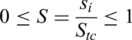
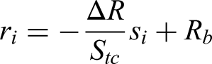
Parameters defining a truncated conical shell are given in Figure 2. The analysis is similar, but not the same as that for a solid truncated cone presented in.² The mapping of pseudo-random numbers in the unit interval, (Ra_s, Ra_φ) _i are used to specify random points on the truncated conical shell, (z_i, r_i, φ_i). For the truncated cone, the axial coordinate dependency on pseudo-random numbers, is derived from the probability density function (PDF) for z directly. For a truncated conical shell, it is more useful to work with the co-ordinate s, defined by the curved surface of the truncated conical shell, as it allows more axisymmetric shapes to be defined as limiting cases of a truncated conical shell, see Figure 2. Considering the coordinate, s, as s increases, the circumference of the hoop on the surface of the shell, decreases linearly. This means that the PDF for s is,

R a_{s} = \frac{\int_{0}^{s_{i}} 2 π r d s}{\int_{0}^{S_{t c}} 2 π r d s}

(5)

Figure 2.

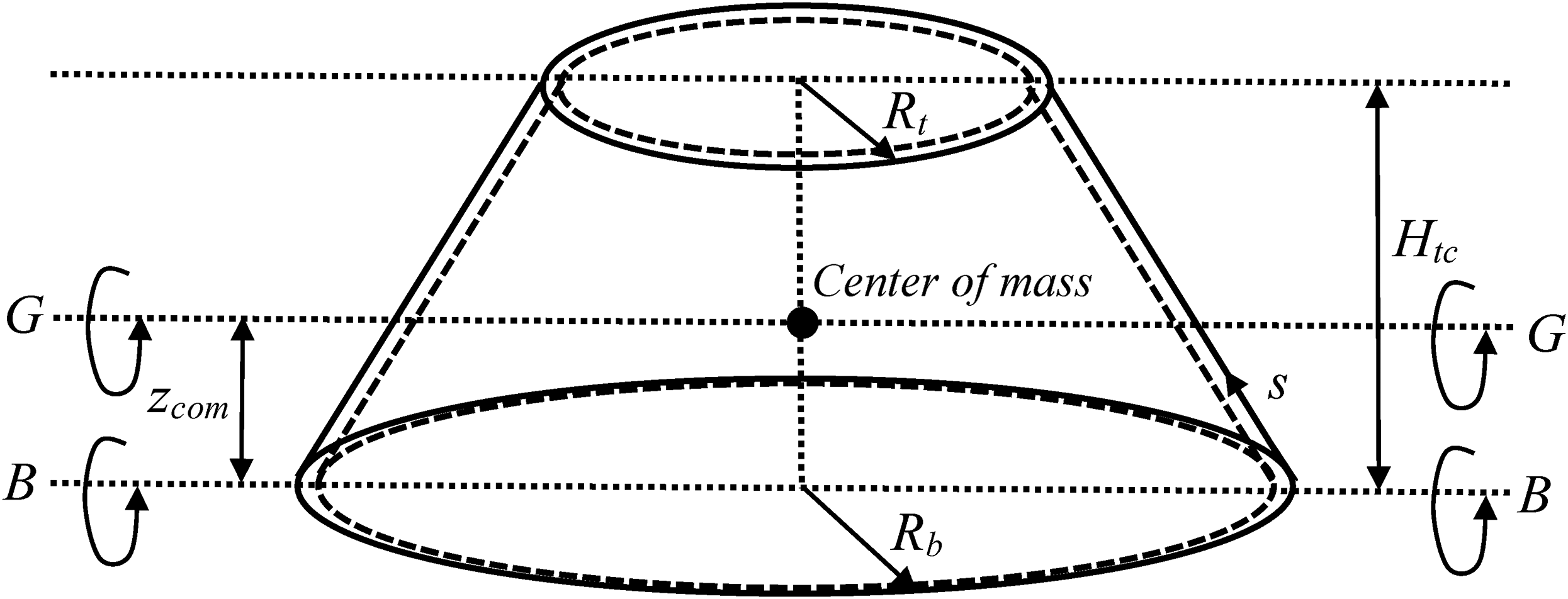
Parameters defining a truncated conical shell.

Where,

S_{t c} = \sqrt{H_{t c}^{2} + {(Δ R)}^{2}}

Δ R = R_{b} - R_{t}

and noting that

r = - \frac{Δ R}{S_{t c}} s + R_{b}

(6)

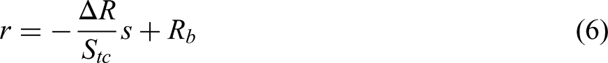
substituting (6) into (5), integrating and rearranging gives the quadratic,

q (S) = \frac{Δ R}{\bar{R}} S^{2} - \frac{R_{b}}{\bar{R}} S + R a_{s} = 0

0 \leq S = \frac{s_{i}}{S_{t c}} \leq 1

\bar{R} = \frac{1}{2} (R_{b} + R_{t})

(7)

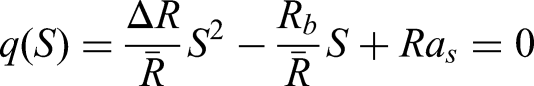
For convenience the coefficients in the quadratic are labelled as,

c (S) = c_{2} S^{2} + c_{1} S + c_{0} = 0

(8)

The two roots of the quadratic are easily found and the root in the unit interval is the correct one to take forward in the analysis.

s_{i} = S_{t c} S_{r o o t}

(9)

The radial co-ordinate and the axial coordinate can be calculated.

r_{i} = - \frac{Δ R}{S_{t c}} s_{i} + R_{b}

z_{i} = \frac{H_{t c}}{S_{t c}} s_{i}

The shape is axisymmetric about the z axis, thus the PDF is uniform and the relationship between the angle φ with respect to the x axis and the pseudo-random number Ra_φ is,

φ_{i} = 2 π R a_{φ}

(10)

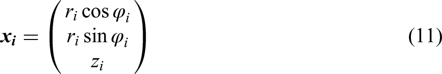
The point vector in Cartesian coordinates is,

x_{i} = (\begin{matrix} r_{i} \cos φ_{i} \\ r_{i} \sin φ_{i} \\ z_{i} \end{matrix})

(11)

The perpendicular distance from x_i to the axis of rotation B-B, is calculated using vector analysis. The equation of a line defined by the axis of rotation, B-B is λn_x where λ is a free parameter, and the direction vector n_x is the unit vector in the x axis direction. The value for λ is calculated by considering the vector x_i -λn_x. The vector x_i -λn_x is orthogonal to the direction vector n_x when,

(x_{i} - λ n_{x}) . n_{x} = 0 \Rightarrow λ = x_{i}

(12)

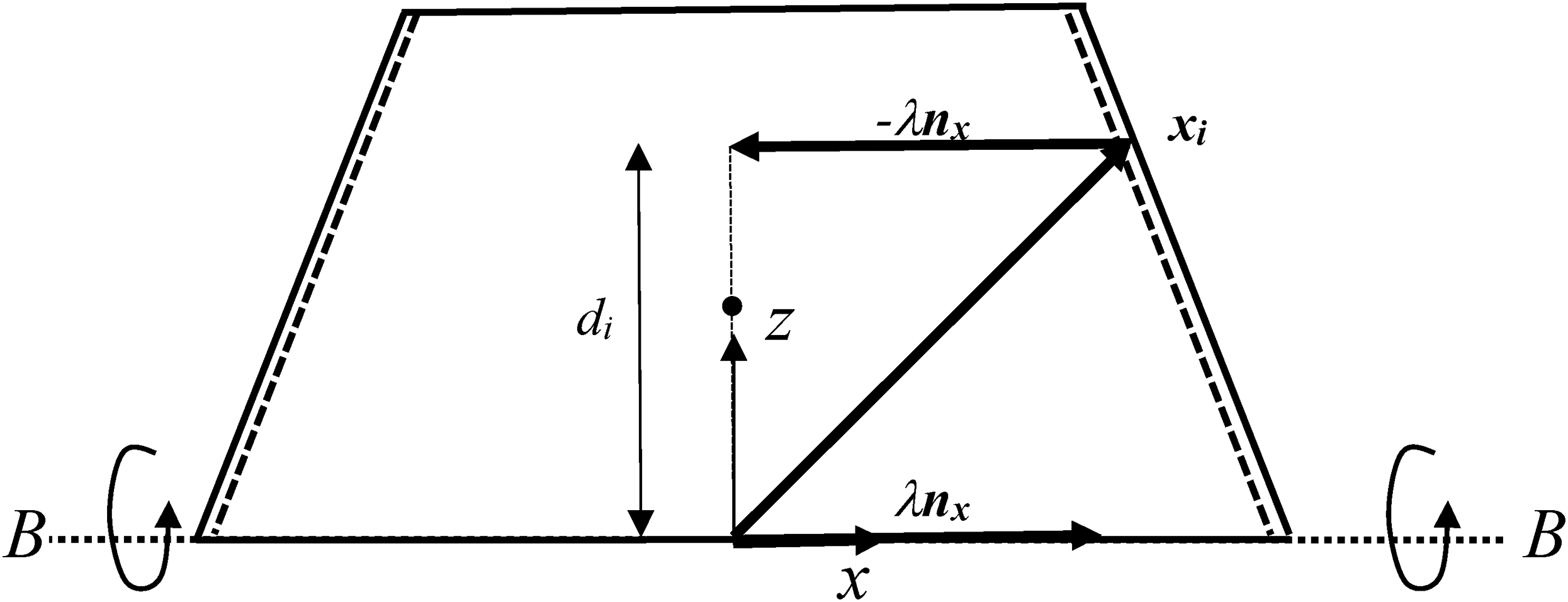
This operation projects the line segment defined by the point vector x_i on to the plane, x = 0 and calculates the length of the projected line segment, see Figure 3.

Figure 3.

Projection of a truncated conical shell onto the plane y = 0, showing the calculation of perpendicular distance for a point and the axis of rotation B-B.

The perpendicular distance squared is then,

d_{i}^{2} = (x_{i} - λ n_{x}) . (x_{i} - λ n_{x})

(13)

The approximate mass moment of inertia for the truncated conical shell using the No PAT method is,

{\tilde{f}}_{N} = \frac{1}{N} \sum_{i = 1}^{N} d_{i}^{2}

I_{B B, t c, N} = m {\tilde{f}}_{N}

(14)

To extend the above analysis for the PAT method. The Monte-Carlo method is applied to calculate I_GG,tc, where G-G is a line parallel to B-B through the center of mass. The center of mass relative to the base is given by

z_{c o m, t c} = H_{t c} (\frac{\frac{1}{2} R_{b} - \frac{1}{3} Δ R}{R_{b} - \frac{1}{2} Δ R}) = \frac{H_{t c}}{3} (\frac{R_{b} + 2 R_{t}}{R_{b} + R_{t}})

(15)

The mapping from pseudo-random numbers, to points on the truncated conical shell is modified to,

z_{i} * = z_{i} - z_{c o m, t c}

x_{i} = (\begin{matrix} r_{i} \cos φ_{i} \\ r_{i} \sin φ_{i} \\ z_{i} * \end{matrix})

(16)

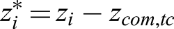
The above modifications, to the analysis allow I_GG,tc to be evaluated, using the Monte-Carlo method. The mass moment of inertia, I_BB,tc is calculated by applying the parallel axis theorem.

I_{B B, t c} = I_{G G, t c} + m z_{c o m}^{2}

(17)

Approximating the MMoI for other axisymmetric shells

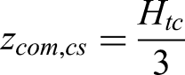
In the appendix, the derivation of the mass moment of inertia for I_BB,tc and I_GG,tc are given as,

I_{B B, t c} = m [\frac{1}{4} (R_{b}^{2} + R_{t}^{2}) + \frac{1}{6} H_{t c}^{2} {\frac{R_{b} + 3 R_{t}}{R_{b} + R_{t}}}]

(18)

I_{G G, t c} = I_{B B, t c} - m z_{c o m, t c}^{2}

(19)

By taking certain limiting values defining the truncated conical shell, other axisymmetric shapes can be represented by the above expressions, and the Monte-Carlo basis can also be applied to the other shapes, with no modification.

The list of possible shapes with appropriate values for R_b, R_t and H_tc are; a conical shell, a tube, a disc, and an annulus. Using the addition property of mass moments of inertia, a composite of truncated conical shells can approximate a hemispherical shell, and a spherical shell. The equations (18, 19) are applicable to all these shapes without modification. Without loss of generality (18, 19) are applicable for all values of R_b and R_t, for the Monte-Carlo method the only restriction is that R_b ≠ R_t. Note the strategy adopted, is to maintain the logic, and modify the parameters to produce approximate mass moments of inertia, with a negligible difference from the correct mass moment of inertia, rather than introduce branches into the logic to account for the separate shapes.

Conical shell specification

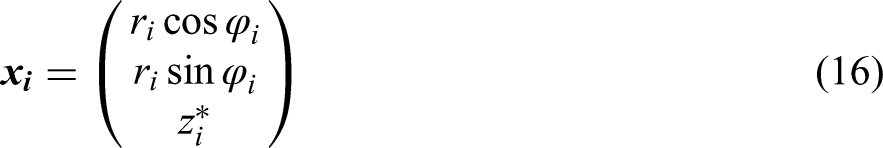
For a conical shell the parameter values are given as R_b = R_cone, R_t = 0 and H_tc = H_cone, with these values the analysis produced for a conical shell is the same as for a truncated conical shell.

I_{B B, c s} = m [\frac{1}{4} R_{b}^{2} + \frac{1}{6} H_{t c}^{2}]

z_{c o m, c s} = \frac{H_{t c}}{3}

I_{G G, c s} = m [\frac{1}{4} R_{b}^{2} + \frac{1}{18} H_{t c}^{2}]

(20)

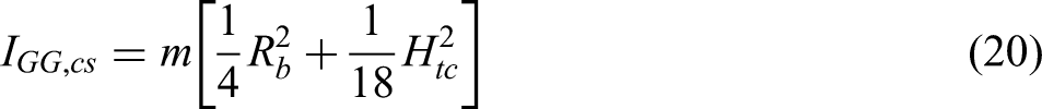
Where I_BB,cs is the MMoI for a conical shell.

Tube specification

For a tube, the parameter values are set to R_b = R_tube, R_t = R_b-ε and H_tc = H_tube. This will produce an approximate mass moment of inertia using the truncated cone analysis. The parameter ε is positive, and indicates a small perturbation of the base radius to ensure that $R_{b} > R_{t}$ . It is not possible to determine the sensitivity of the mass moment of inertia to the value of ε analytically. This is investigated numerically below. Note if the strategy of setting the top radius to the bottom radius of the truncated conical shell, then (8) reduces to a linear equation and the truncated cone analysis would have to be modified.

I_{B B, t u b e, t c} = m (\frac{1}{2} R_{b}^{2} + \frac{1}{3} H_{t c}^{2}) + O (ε) = I_{B B, t u b e} + O (ε)

z_{c o m, t u b e, t c} = \frac{H_{t c}}{2} + O (ε) = z_{c o m, t u b e} + O (ε)

I_{G G, t u b e, t c} = m (\frac{1}{2} R_{b}^{2} + \frac{1}{12} H_{t c}^{2}) + O (ε) = I_{G G, t u b e} + O (ε)

(21)

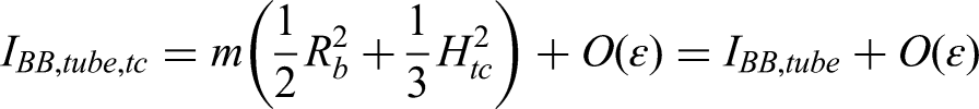
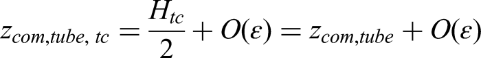
Where I_BB,tube,tc is the MMoI for a truncated conical shell approximating a tube.

2-Dimensional disc

For a 2-dimensional disc the parameter values are set to, R_b = R_disc, R_t = 0 and H_tc=0. The mass moment of inertia for a truncated conical shell is exact for a disc. Applying the Monte-Carlo methods, the No PAT method and PAT method described above, can be applied directly to the representation of a disc, as the co-ordinate of the curved surface of the truncated conical shell, s is applicable without modification.

I_{B B, d i s c, t c} = \frac{m}{4} R_{b}^{2} = I_{G G, d i s c}

(22)

2-Dimensional Annulus

For a 2-dimensional annulus, the parameter values are set to, R_b = R_o, R_t = R_i and H_tc=0. The mass moment of inertia for a truncated conical shell is exact for an annulus. Applying the Monte-Carlo method, the No PAT method and PAT method, described above can be applied directly, to the representation of an annulus as the co-ordinate of the curved surface of the truncated conical shell, s is applicable without modification.

I_{B B, a n n u l u s, t c} = \frac{m}{4} (R_{b}^{2} + R_{t}^{2}) = I_{G G, a n n u l u s}

(23)

Hemispherical shell and spherical shell

Any axisymmetric shell, can be approximated as a composite of truncated conical shells. For example, for a hemispherical shell, it can be partitioned into a conical shell at the apex of the hemisphere, and (n-1) truncated conical shells below it, see Figure 4. The bigger n is, the more accurate the representation of the hemispherical shell. The same approximation with 2 conical shells for the top and bottom of the spherical shell, and (n-2) truncated conical shells between them also works. An appropriate value for n must be chosen. The conical shells are modelled as truncated conical shells with R_t = 0. The approximate mass moment of inertia is then,

I_{B B, c o m p} = \sum_{i = 1}^{N_{t c}} I_{B B, t c, i}

(24)

Figure 4.

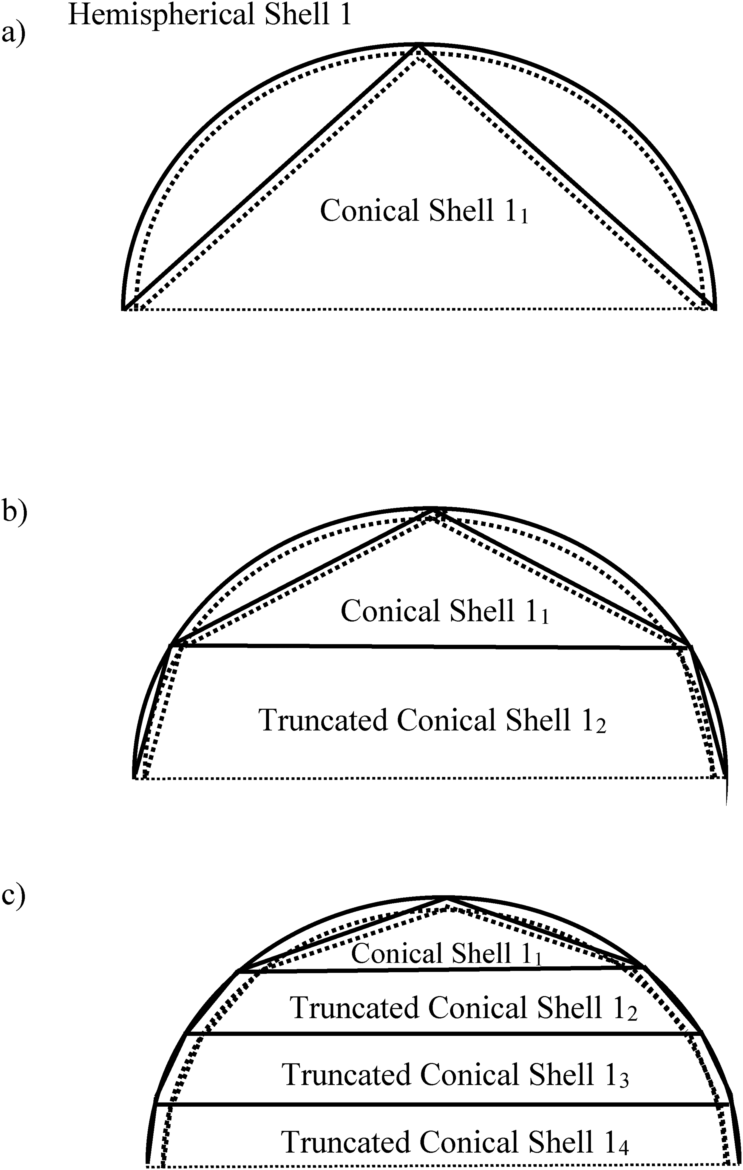
Different partitions of a hemispherical shell using truncated conical shells and a single conical shell, a) 1 partition, b) 2 partitions, c) 4 partitions.

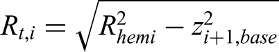
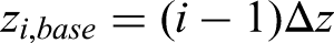
Where N_tc is the number of truncated conical shells. The parameters for each truncated conical shell are,

Δ z = \frac{R_{h e m i}}{N_{t c}}

R_{b, i} = \sqrt{R_{h e m i}^{2} - z_{i, b a s e}^{2}}

i = 1, 2, \dots, N_{t c}

R_{t, i} = \sqrt{R_{h e m i}^{2} - z_{i + 1, b a s e}^{2}}

z_{i, b a s e} = (i - 1) Δ z

H_{t c} = Δ z

(25)

Application of the Monte-Carlo method to calculating MMoI

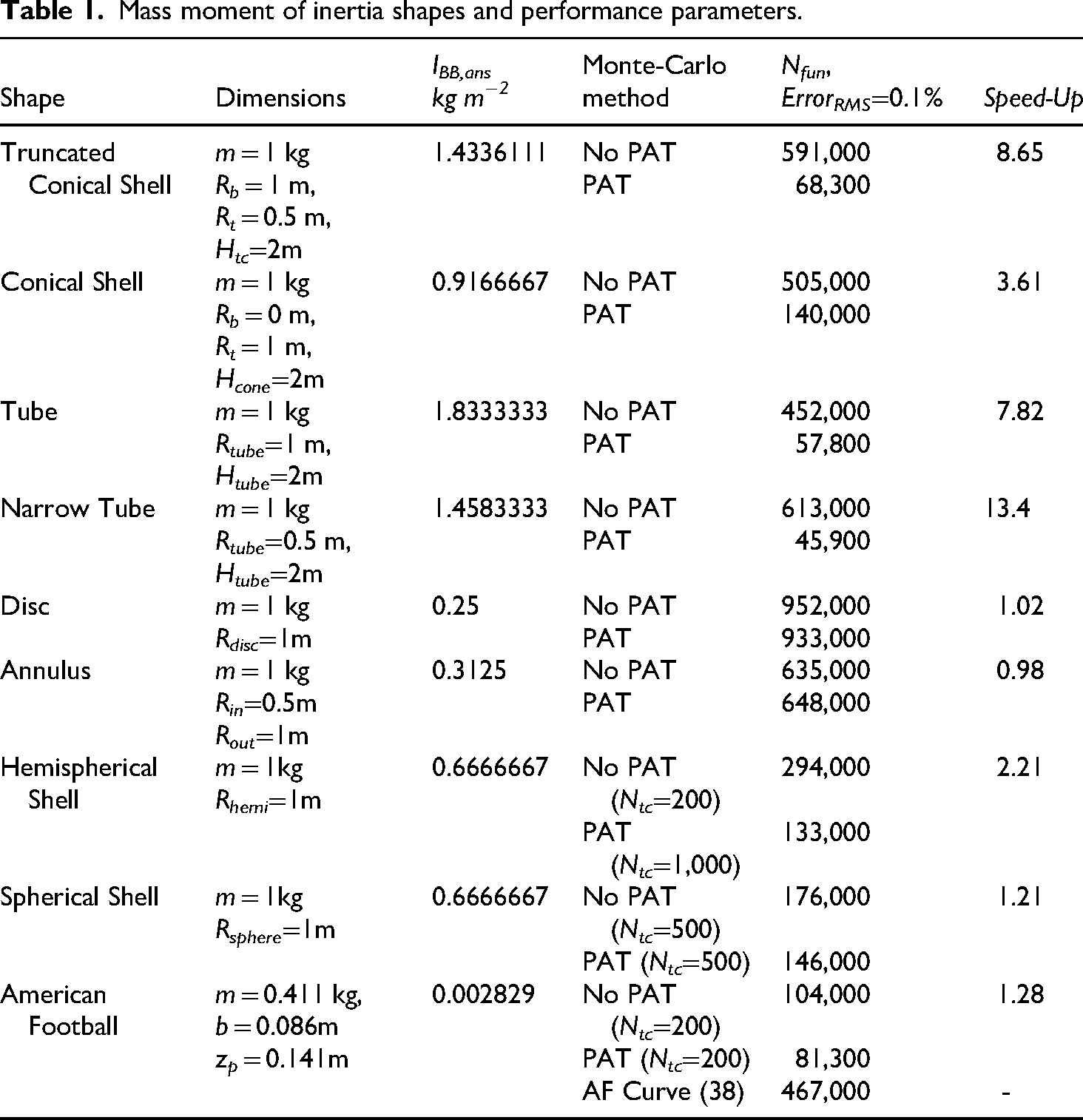
In this section, the two Monte-Carlo methods are evaluated, by considering a number of axisymmetric shells and 2-dimensional axisymmetric shapes. The test problems chosen to evaluate the Monte-Carlo methods mirror the test problems considered in the linked paper.² The No PAT method, and PAT method can be evaluated, for the evaluation of MMoI of axisymmetric shells, and compared to the performance of the two methods, applied to axisymmetric solid shapes considered in.² The parameters defining each of the shapes are given in Table 1. The first shape considered is a truncated conical shell.

Table 1.

Mass moment of inertia shapes and performance parameters.

Shape	Dimensions	I_BB,ans kg m⁻²	Monte-Carlo method	N_fun, Error_RMS=0.1%	Speed-Up
Truncated Conical Shell	m = 1 kg R_b = 1 m, R_t = 0.5 m, H_tc=2m	1.4336111	No PAT	591,000	8.65
Truncated Conical Shell	m = 1 kg R_b = 1 m, R_t = 0.5 m, H_tc=2m	1.4336111	PAT	68,300	8.65
Conical Shell	m = 1 kg R_b = 0 m, R_t = 1 m, H_cone=2m	0.9166667	No PAT	505,000	3.61
Conical Shell	m = 1 kg R_b = 0 m, R_t = 1 m, H_cone=2m	0.9166667	PAT	140,000	3.61
Tube	m = 1 kg R_tube=1 m, H_tube=2m	1.8333333	No PAT	452,000	7.82
Tube	m = 1 kg R_tube=1 m, H_tube=2m	1.8333333	PAT	57,800	7.82
Narrow Tube	m = 1 kg R_tube=0.5 m, H_tube=2m	1.4583333	No PAT	613,000	13.4
Narrow Tube	m = 1 kg R_tube=0.5 m, H_tube=2m	1.4583333	PAT	45,900	13.4
Disc	m = 1 kg R_disc=1m	0.25	No PAT	952,000	1.02
Disc	m = 1 kg R_disc=1m	0.25	PAT	933,000	1.02
Annulus	m = 1 kg R_in=0.5m R_out=1m	0.3125	No PAT	635,000	0.98
Annulus	m = 1 kg R_in=0.5m R_out=1m	0.3125	PAT	648,000	0.98
Hemispherical Shell	m = 1kg R_hemi=1m	0.6666667	No PAT (N_tc=200)	294,000	2.21
Hemispherical Shell	m = 1kg R_hemi=1m	0.6666667	PAT (N_tc=1,000)	133,000	2.21
Spherical Shell	m = 1kg R_sphere=1m	0.6666667	No PAT (N_tc=500)	176,000	1.21
Spherical Shell	m = 1kg R_sphere=1m	0.6666667	PAT (N_tc=500)	146,000	1.21
American Football	m = 0.411 kg, b = 0.086m z_p = 0.141m	0.002829	No PAT (N_tc=200)	104,000	1.28
			PAT (N_tc=200)	81,300	1.28
			AF Curve (38)	467,000	-

Truncated conical shell

A truncated conical shell, is defined to have a mass of m = 1 kg, a base radius of R_b = 1 m, a top radius of R_t = 0.5 m, and the height H_tc varies from 0.25 m to 2 m step 0.25 m, see Figure 2. The estimates of I_BB,tc are evaluated, using the No PAT method and PAT method, with N_fun=100 function evaluations. Figure 5, shows I_BB,tc curves, calculated using the two Monte-Carlo methods and the analytical solution, (18). As H_tc increases the MMoI increases, as expected. Comparing the two Monte-Carlo methods the PAT method looks to be marginally more accurate than the No PAT method. The difference between the two methods, is less than that demonstrated for the solid truncated cone test problem, with the same defining parameters, see Figure 5 in.² For the truncated conical shell, the average relative error for the No PAT method and the PAT method are 4.2% and 5.1% respectively.

Figure 5.

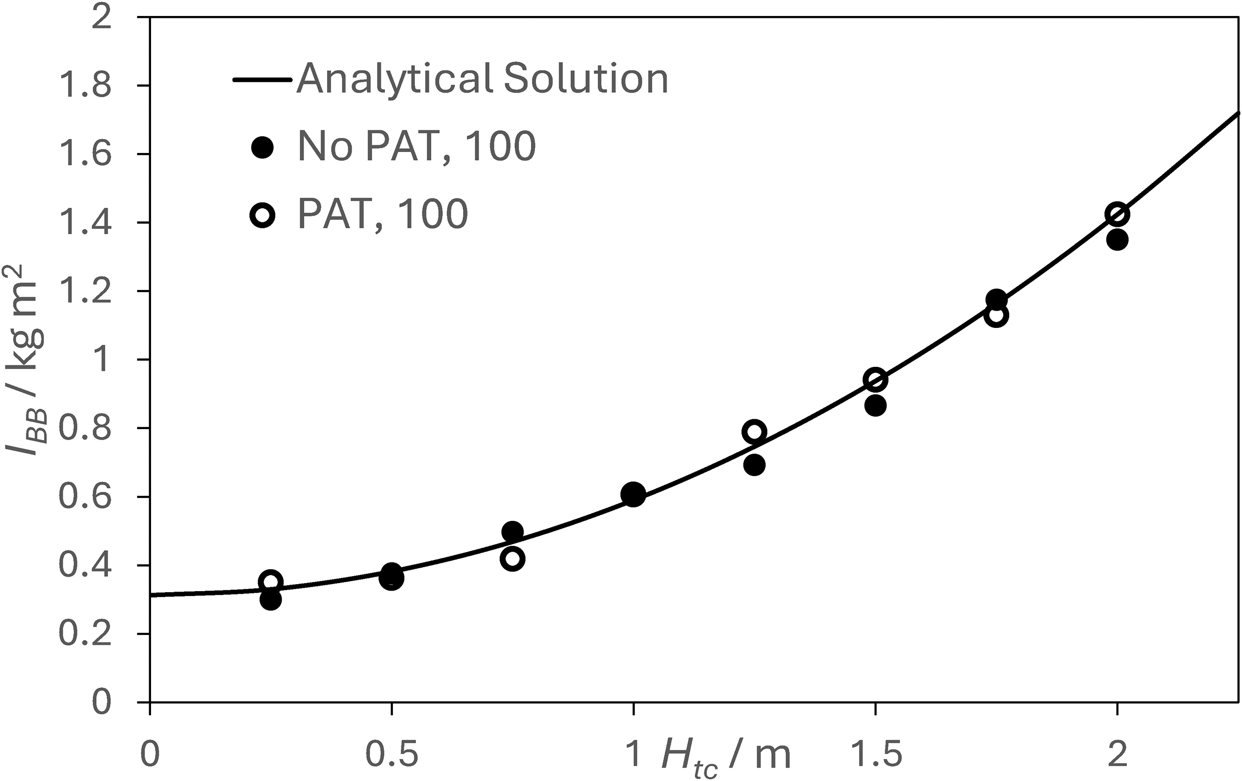
For the truncated conical shell, I_BB vs. H_tc, the analytical solution, and the No PAT and PAT method predictions for N_fun=100.

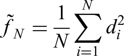
Defining the root mean squared relative error, Error_RMS as,

E r r o r_{R M S} (N_{f u n}) = \frac{100}{I_{B B, a n s}} \times \sqrt{\frac{1}{N_{s a m p l e}} \sum_{i = 1}^{N_{s a m p l e}} {(I_{B B, a n s} - I_{B B, i})}^{2}}

I_{B B, i} = \frac{1}{N_{f u n}} \sum_{j = 1}^{N_{f u n}} I_{B B, j}

(26)

Where N_sample is the number of realizations of I_BB,tc for a given N_fun. I_BB,j denotes a single realization of the MMoI, and I_BB,i is an estimate of MMoI calculated with N_fun function evaluations. Twenty samples are sufficient, to give a relatively smooth Error_RMS vs. N_fun curve, N_sample =20. Figure 6, shows the Error_RMS vs. N_fun curve for $10 \leq N_{f u n} \leq 10^{6}$ , for a truncated conical shell with H_tc =2 m, see Table 1. In Figure 6, the axes are logarithmic, and the Error_RMS curves for the No PAT method, and PAT method are shown. The logarithmic axes, mean that a straight line indicates a power law relationship. An additional curve, is also shown in Figure 6, a power law curve with a power law index, n = -0.5. This is included to demonstrate that the Monte-Carlo methods reproduce the expected, n = -0.5 power law relationship for a stochastic process, satisfying the central limit theorem. Considering the No PAT method and PAT method, Error_RMS curves in Figure 6 demonstrate that the PAT method consistently delivers a more accurate estimate of I_BB,tc for any given N_fun. The difference between the two Error_RMS curves, is significant given the Error_RMS axis is logarithmic.

Figure 6.

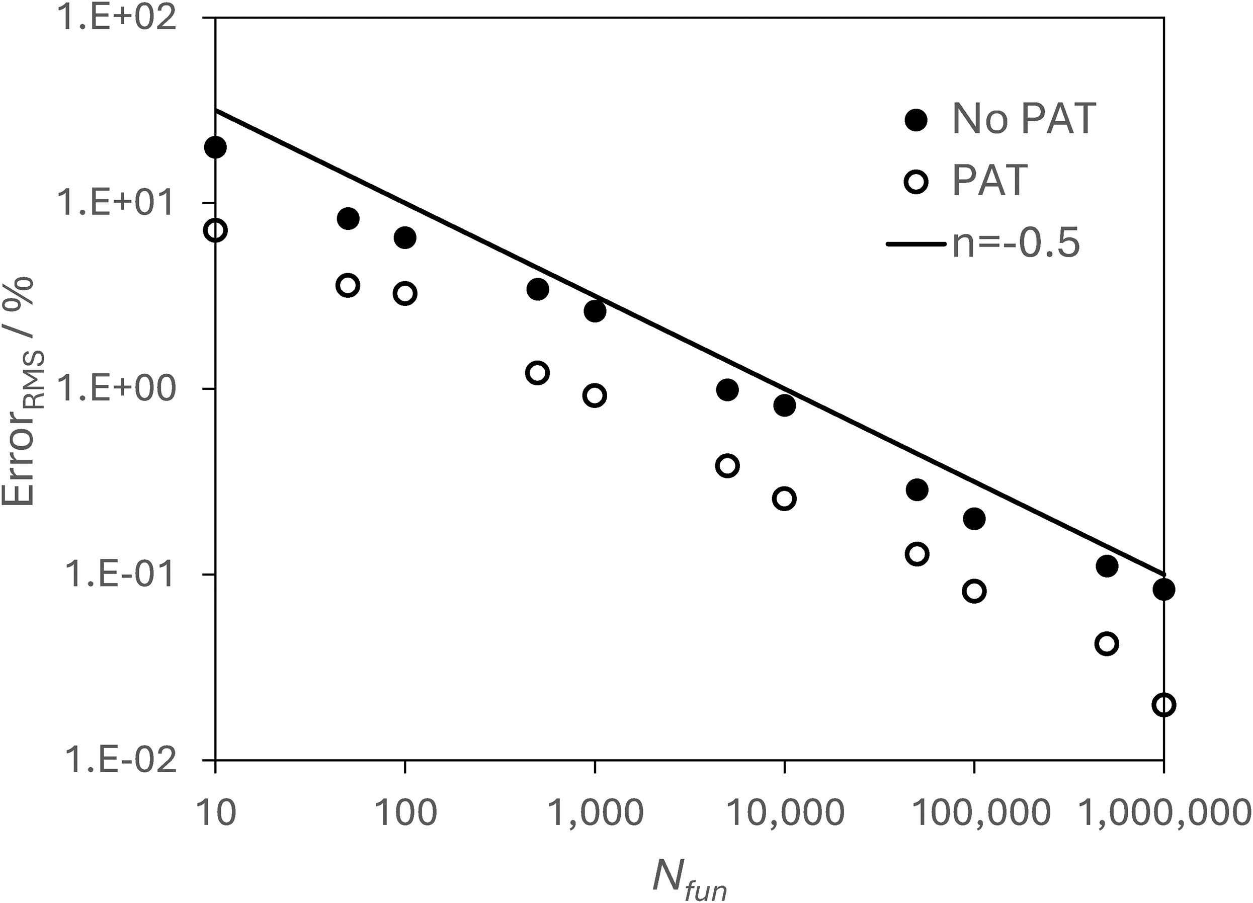
Error_RMS vs. N_fun, for a truncated conical shell, m = 1 kg R_b = 1 m R_t = 0.5 m, H_tc=2 m calculated using the No PAT and PAT method.

To quantify the difference, in the two Error_RMS curves, the number of function evaluations to achieve a relative error Error_RMS =0.1% is used.

N_{f u n, 0.1 %} = a r g {E r r o r_{R M S} (N_{f u n}) = 0.1 %}

(27)

Using Error_RMS =0.1% is an arbitrary value, but it is still useful, and allows a speed up parameter to be defined,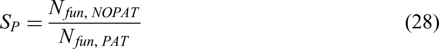

S_{P} = \frac{N_{f u n, N O P A T}}{N_{f u n, P A T}}

(28)

For the truncated conical shell, the MMoI calculated using the No PAT method with an accuracy of Error_RMS =0.1% is N_fun,0.1% = 591,000 and for the PAT method N_fun,0.1% = 68,300. This gives a speed-up value of S_P = 8.65. All of the data for this test problem are summarized in Table 1.

Tube

The second shell-like shape considered in this investigation is the MMoI of a tube with axis of rotation through its base perpendicular to the tube. The tube is defined by the parameters, m = 1 kg, R_tube = R_b = 1 m, R_t = R_b-ε, H_tube = H_tc=2 m, see Table 1. An analogous calculation for a solid cylinder, with the same defining parameters is considered in.² The parameter ε needs to be given an appropriate value. To determine ε, a number of No Pat method MMoI simulations with N_fun=10⁷ and $10^{- 8} \leq ε \leq 0.2$ are calculated. The number of function evaluations, is sufficiently large such that a significant component of the numerical error, relates to the approximate representation of a tube, determined by ε. Figure 7(a), shows the No PAT method calculations of I_BB,tc vs. ε together with the exact value, I_BB,tube=1.8333333 kg m². To the resolution of the figure, for $ε \leq 10^{- 3}$ the No PAT method estimate of the MMoI has negligible numerical error. A similar comparison, for the PAT method indicates similar behavior. Therefore, the value of ε=10⁻⁷, is used in all remaining MMoI calculations.

Figure 7.

For the tube shape, a) I_BB,tc vs. ε, for the No PAT method, with N_fun=10⁷ and the analytical solution and b) Error_RMS vs. N_fun for the No PAT and PAT method for I_BB,tc and a power law curve with index n = -0.5.

Figure 7(b), shows a comparison of the Error_RMS vs. N_fun for the tube, using the No PAT method and the PAT method together with a power law curve, with power law index n = -0.5. The behavior is similar to that exhibited in Figure 6, for the truncated conical shell. For the tube, the number of function evaluations to achieve Error_RMS=0.1% for the No PAT method and the PAT method are N_fun,0.1% = 452,000 and N_fun,0.1% = 57,800 respectively. This gives a speed-up of S_P = 7.82.

A similar set of calculations have been completed for a narrow tube defined by the parameters m = 1 kg, R_tube = R_b = 0.5 m, R_t = R_b-ε, H_tube = H_tc=2 m. The number of function evaluations to achieve an error, Error_RMS=0.1% for the No PAT method and the PAT method are N_fun,0.1%=613,000 and N_fun,0.1%=45,900 respectively. For the narrow tube shape the speed-up is S_P = 13.4. The speed-up for the PAT method, increases as the aspect ratio (H_tube/R_tube) of the tube increases, as the integral kernel variation for the MMoI I_GG,tc is less than the variation for the MMoI for I_BB,tc. This situation has been analyzed for a rod in.² If the internal kernel of (1) for a 1-dimensional shape is denoted f, then the variance for a function is

V a r (f) = E (f^{2}) - E (f)^{2}

(29)

The smaller the variance, the fewer function evaluations are required to achieve an accurate value, for the mean of the integral kernel. The extreme case, is for a constant integral kernel the variance is zero, and one function evaluation gives the exact mean for the integral kernel.

Hemispherical shell

In this sub-section, the Monte-Carlo method, is applied to the MMoI of a hemispherical shell, with an axis of rotation through the base. The parameters defining the hemispherical shell are, m = 1 kg and R_hemi = 1 m. The solution strategy, is to represent the hemispherical shell as a composite of truncated conical shells (24). For the truncated conical shell, at the apex of the hemispherical shell R_t = 0. The approximation to the mass moment of inertia I_BB,hemi, is given as the summation,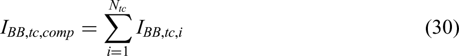

I_{B B, t c, c o m p} = \sum_{i = 1}^{N_{t c}} I_{B B, t c, i}

(30)

For this shape, the number of truncated conical shells, N_tc needs to be sufficiently large.

Figure 8(a), shows the calculated MMoI using the No PAT method and the PAT method. Each of the calculated MMoI, is evaluated with N_fun,total=10⁷, such that the dominant component of the numerical error, is associated with the representation of the hemispherical shape, N_tc. In Figure 8(a), the Monte-Carlo method evaluation of the MMoI is plotted against N_tc, $1 \leq N_{t c} < 100$ . The exact value for the MMoI, is also indicated in Figure 8(a), I_BB,hemi=2/3 kg m². The PAT method, requires fewer truncated conical shells to represent the hemispherical shell accurately, compared to the No PAT method. The PAT method, requires $N_{t c} \geq 20$ to produce an estimate of the MMoI, that is negligibly different to the exact value, to the resolution of Figure 8(a). For the No PAT method a much finer discretisation of the hemispherical shell is required to achieve a similar degree of accuracy as the PAT method. For the No PAT method, $N_{t c} \geq 90$ to achieve a similar numerical accuracy, as exhibited by the PAT method. This is interesting, but not a significant issue for determining the numerical accuracy of the No PAT method. Assuming an appropriate value for N_tc is determined, it places a constraint on the number of function evaluations, as efficiency considerations of the Monte-Carlo method requires that N_fun,total, the total number of function evaluations can be factorized as,

N_{f u n, t o t a l} = N_{f u n} N_{t c}

(31)

Figure 8.

For the hemispherical shell a) I_BB,tc, vs. N_tc, for the No PAT method and PAT method, with N_fun=10⁷ and the analytical solution and b) Error_RMS vs. N_fun, for the No PAT and PAT method and a power law curve with index n = -0.5.

Figure 8(b), shows a comparison of the Error_RMS vs. N_fun,total for the No PAT method, and the PAT method, as well as the power law curve with a power law index n = -0.5. For the No PAT method, the hemispherical shell is represented as N_tc=1,000 truncated conical shells and for the PAT method N_tc=200. These values for N_tc were determined, to ensure that it is possible to calculate an Error_RMS curve, such that the number of function evaluations to achieve Error_RMS =0.1% is possible. The PAT method is marginally more accurate than the No PAT method. The No PAT method Error_RMS curve plateaus for N_fun,total≥10⁶ at a value of Error_RMS just below 0.1%. If a more accurate value for Error_RMS is required, then N_tc would have to be increased. The number of function evaluations to achieve an error of Error_RMS =0.1% for the No PAT method, and the PAT method are N_{fun,total,0.1%}=294,000, and N_{fun,total,0.1%}=133,000 respectively. This gives a speed up of S_P = 2.21.

Conical shell, spherical shell, disc and annulus

The shapes considered in this sub-section are; a conical shell, a spherical shell, a disc, and an annulus. Each of the shapes defining parameters are given in Table 1. The different Monte-Carlo methods, the No PAT method, and the PAT method are evaluated, using N_fun,0.1%, the number of function evaluations to achieve an error of Error_RMS=0.1%. For the conical shell, the No PAT method and the PAT method are N_fun,0.1%=505,000 and N_fun,0.1%=140,000 respectively, and the speed up parameter is S_P = 3.61.

For the other three shapes the PAT method either has a similar performance to the No PAT method or is marginally superior. For the disc, and annulus, z_com=0 and theoretically I_BB = I_GG. Any differences in the data presented in Table 1, for these two shapes are associated with stochastic effects.

Taking the MMoI of the shapes, that can be defined as a limiting case of a truncated conical shell, or truncated cone² suggests that in general the PAT method tends to be more efficient than the No PAT method provided z_com>0. It is difficult to quantify the likely improvement in efficiency, of the PAT method compared to the No PAT method, except that the greater z_com is, the more likely the improvement is significant. It is now possible, to apply the analysis presented here, and in² to evaluate the mass moment of inertia, of any axisymmetric shape. This is considered further in the next section.

Examples of student projects for the calculation of MMoI of axisymmetric bodies

The Monte-Carlo methods developed for the calculation of axisymmetric shapes, are quite complicated to derive, and are beyond most undergraduate mechanical engineering students, except for the most able. The educational value of this investigation, is that once the Monte-Carlo method calculation of the MMoI of a truncated cone and truncated conical shell is implemented, then a student can take the software and compute the MMoI of any axisymmetric shape, in any field of engineering of interest to them. This means that students can be given instructions to find an axisymmetric shape in a field of engineering of interest to them. The student can then complete a numerical experimental investigation using the Monte-Carlo method, to calculate the MMoI of the axisymmetric shape.

In this section, two examples are given, of what a student project might look like, one taken from rocket design and a second taken from sports science.

Estimating the MMoI of a Saturn V rocket (Apollo 10)

The Saturn V rocket is a 3-stage rocket, for launching the Apollo missions to the moon, in the late 1960s and early 1970s. The rocket is 111 m tall, and at launch the mass of the rocket, propellant and payload is approximately $2.9 \times 10^{6}$ kg.

The rocket has three stages. Stage S-IC, the first stage has five rocket engines. On ignition all five rocket engines are powered up. After 2 min, 15 s the central engine is switched off. This is done to limit acceleration to less than 4.5 g. The four remaining engines deliver full thrust up to a time of 2 min, 41 s after launch. At this point, the first stage separates and the second stage, Stage S-II has five rocket engines delivering full thrust up to a time of 7 min, 39 s after launch. At this time, the center engine is switched off to limit acceleration. The remaining four engines continue to produce thrust until a time of 9 min 14 s after launch. The second stage is then jettisoned. The final third stage, Stage IVB has a single rocket engine. The third stage engine ignition occurs at 11 min, 14 s after launch. The stage IVB engine is switched off at a time of 11 min 53 s, when the Saturn V rocket is put into a parking orbit approximately 185 km above the earth's surface, before the Saturn V rocket engine sometime later moves on to the second part of the mission to orbit the moon.

The objective of the student project, is to approximate the mass and mass distribution of the Saturn V rocket for the time between launch and achieving a parking orbit around the earth. The Saturn V rocket is shown in Figure 9. The itinerary of components of a Saturn V rocket is documented in some detail.^3,19 There are too many structures / equipment to be defined individually, in an approximation of the mass distribution, to calculate the MMoI of the Saturn V rocket. The simplest representation of the mass distribution to represent a Saturn V rocket is 7 components. Stage S-IC is approximated to be a cylindrical shell surrounding a cylinder of propellant. The rocket fuel and liquid oxygen are considered as a single fluid, the propellant, and is modelled as a solid cylinder with the mass of propellant reducing with time. Stage S-II is represented as a cylindrical shell for the main body, and a solid cylinder for the propellant. For Stage S-IVB the main body and propellant have a similar representation to the other two stages. The final component of the Saturn V idealized representation, the command module / payload is modelled as a cylindrical shell, on top of the Stage S-IVB. All the dimensions of the rocket stage defining parameters, are stated in the Apollo 10 Technical Information Summary.³ The propellant tanks have the same mass as stated in the summary document, but the fuel/oxygen tanks are assumed homogeneous and have a cylindrical shape, with the correct mass and volume. The location and dimension of the seven idealized components of the Saturn V rocket are given in Table 2. The location of the base of each component relative to the base of the rocket is shown in Figure 9.

Figure 9.

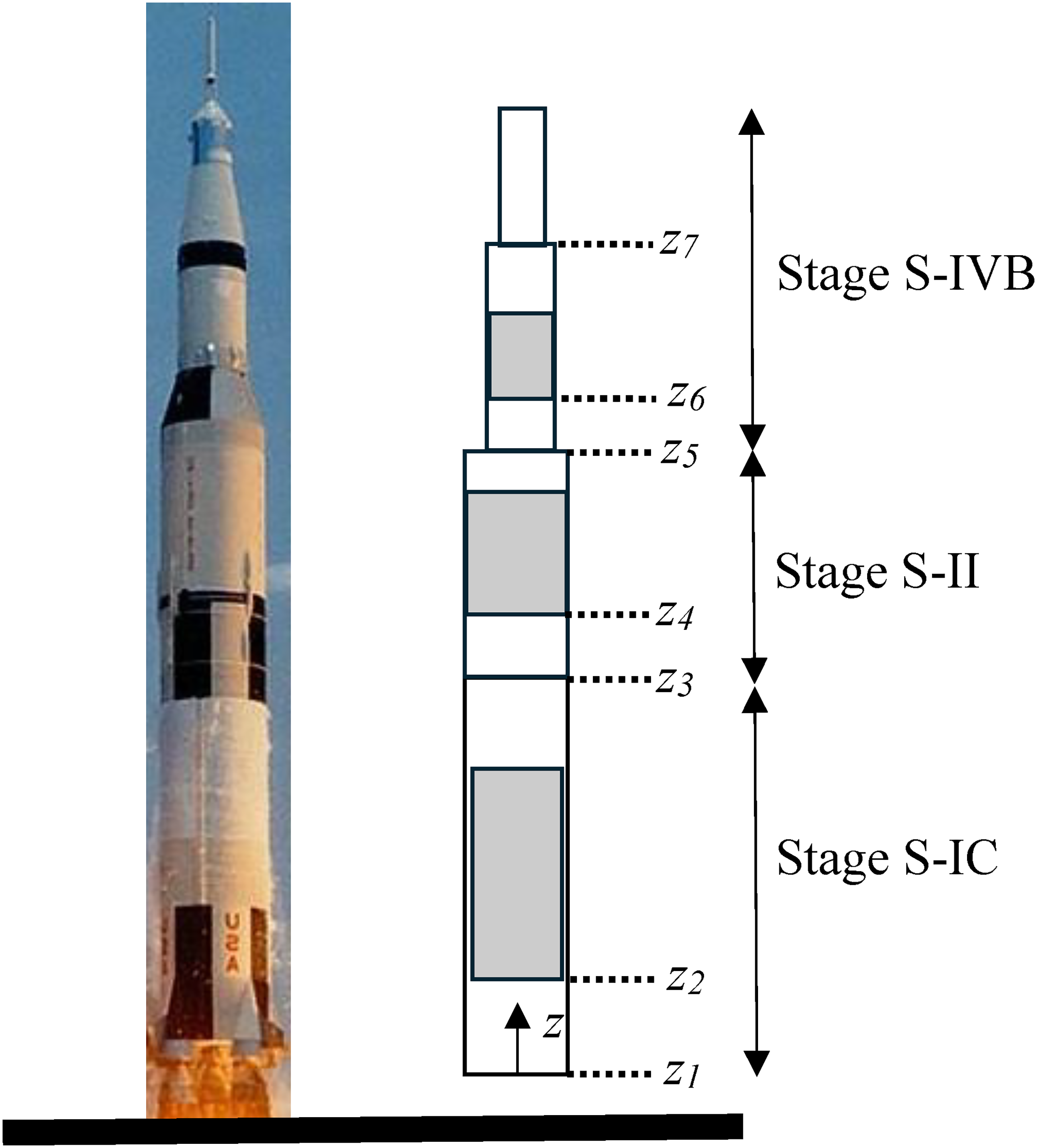
Saturn V rocket*,³ and a seven-component approximation to a Saturn V rocket.

Table 2.

Saturn V rocket dimensions

Component	Name	Shape	m/kg	Z_com/m	Z_base / m	R/m	H/m
1	Stage S-IC Shell	Cylindrical Shell	134,000	19.1	0	5.1	38.2
2	Stage S-IC Propellant	Solid Cylinder	2,148,000*	20.95	5	4.6	31.9
3	Stage S-II Shell	Cylindrical Shell	38,400	50.7	38.2	5.1	25
4	Stage S-II Propellant	Solid Cylinder	446,000*	50.1	43.2	5.1	13.8
5	Stage S-IVB Shell	Cylindrical Shell	18,500	73.7	63.2	3.3	21
6	Stage S-IVB Propellant	Solid Cylinder	122,000*	73.7	68.2	3.3	11
7	Stage 2-IVB Payload	Cylindrical Shell	24,400	91.25	84.2	2.0	14.1

* Initial Mass.

The mass of the Saturn V rocket for the first 675 s after launch is shown in Figure 10(a). The Stage S-IC/ S-II separation occurs at t = 161 s, and the Stage S-II/ S-IVB separates at t = 555 s. Figure 10(b), shows the center of mass of the Saturn V rocket between launch and achieving a parking orbit around earth.

z_{c o m, r o c k e t} = \frac{\sum_{i = 1}^{7} m_{i} z_{c o m, i}}{\sum_{i = 1}^{7} m_{i}}

(32)

Figure 10.

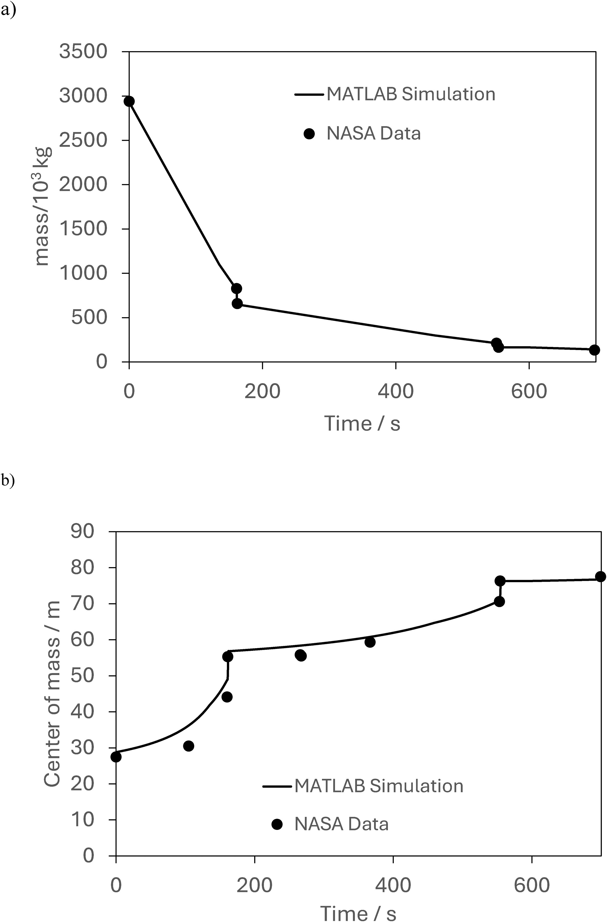
a) Mass of Saturn V rocket vs. time and b) Center of mass of Saturn V rocket vs. time.

The points in Figure 10(b), are the center of mass of the Saturn V rocket given by NASA.³ The full line, is the center of mass, calculated in a MATLAB simulation of the 7 component idealized representation of the Saturn V rocket. Comparing the NASA data with the MATLAB simulation of the center of mass, they are in close agreement with each other. The largest error occurs at t = 105 s, where the relative difference is 15% with a much smaller error for all other times.

The mass moment of inertia for the Saturn V rocket is shown in Figure 11, for $t \leq 150 s$ . Figure 11(a), shows three estimates of the MMoI for the Saturn V rocket, for an axis parallel to the base, through the rockets center of mass, (30). The full line in Figure 11(a), is the analytical curve for the MMoI for the seven-component idealization of the Saturn V rocket. The dotted line in Figure 11(a), is the Monte-Carlo method calculation of the MMoI using the No PAT method with N_fun,total=700, the number of function evaluations per component, N_fun=100. The curve labelled NASA Simulation, Apollo 8 in Figure 11(a), is a NASA calculation of the MMoI.²⁰ There is no equivalent curve available for the Apollo 10 launch, but it is expected to be similar to Apollo 8, for the time interval considered in Figure 11(a). The stochastic nature of the No PAT method MMoI curve is clear in Figure 11(a), with the I_{GG, No PAT} bracketing the exact MMoI curve. The level of agreement of the MMoI calculated using the idealized component representation of the Saturn V rocket and the Apollo 8 NASA simulation is qualitatively, and to some degree quantitively similar. Figure 11(b), shows the No PAT method calculation of I_{GG,No PAT} with N_fun,total =7,000. If a more accurate representation of the MMoI, with a smaller numerical error is of interest, then N_fun,total can be increased.

Figure 11.

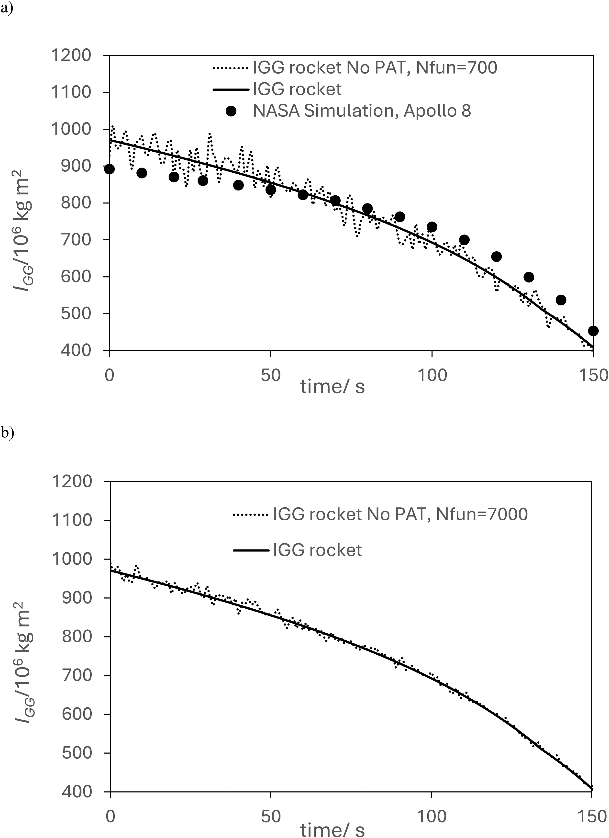
MMoI for the approximate Saturn V rocket shape and a), the no PAT method and a NASA simulation of appollo 8 and b) the PAT method.

By way of comparison between the No PAT method applied to the Saturn V rocket, Figure 12(a), shows the relative error in the MMoI, I_{GG,No PAT} calculated using N_fun,total=700, and N_fun,total =7,000. The maximum relative error for the No PAT method is approximately 9% for N_fun,total =700 and reduces to 3% for N_fun,total =7,000. Figure 12(b), shows a similar relative error curve for the PAT method. The maximum relative error for the PAT method is approximately 4% for N_fun,total =700, and reduces to 1% for N_fun,total =7,000.

Figure 12.

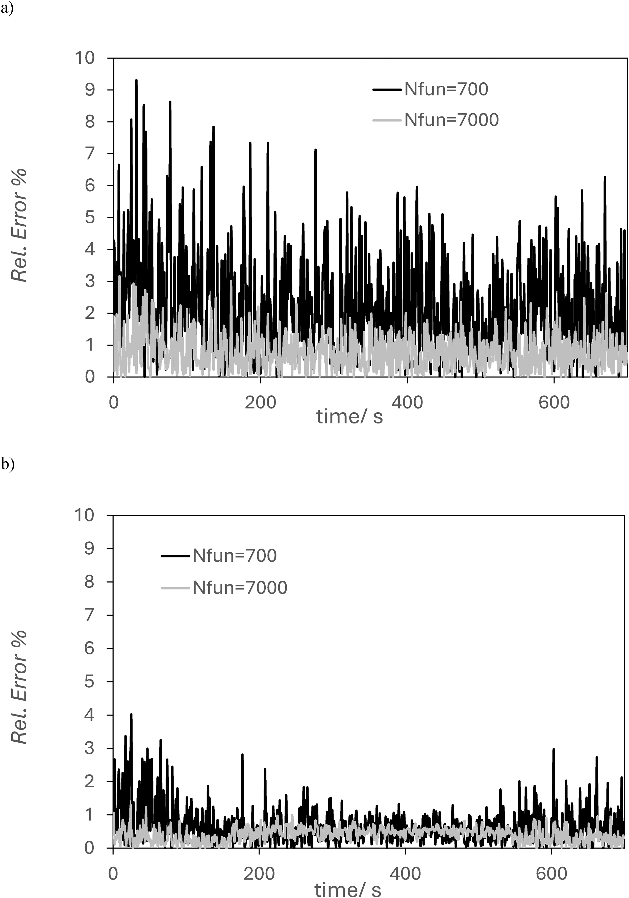
The relative error of the MMoI for a Saturn V rocket for a) the no PAT method, and b) the PAT method.

Calculating the MMoI of an American football

In this section, the mass moment of inertia of an American football, for an axis through its center of mass, parallel to its minor axis is considered, see Figure 13. This is the mass moment of inertia of an American football, required to determine the angular acceleration of the ball, due to a torque applied by the hands of the player. This is of interest due to the seemingly paradoxical dynamic behavior of a thrown American football. Once released by a player, the American football follows a parabolic trajectory. During the flight the major axis of the rotating balls trajectory, tends to remain aligned with the major axis of the ball. This is unexpected, as you might expect the American football to have a tendency to pitch backwards, rotating vertically about its minor axis. The reason for the possible rotation about the minor axis, is because of drag force on the American football inducing a torque, τ_pitch.

τ_{p i t c h} = (z_{C P} - z_{c o m}) \times F_{d r a g}

(33)

Figure 13.

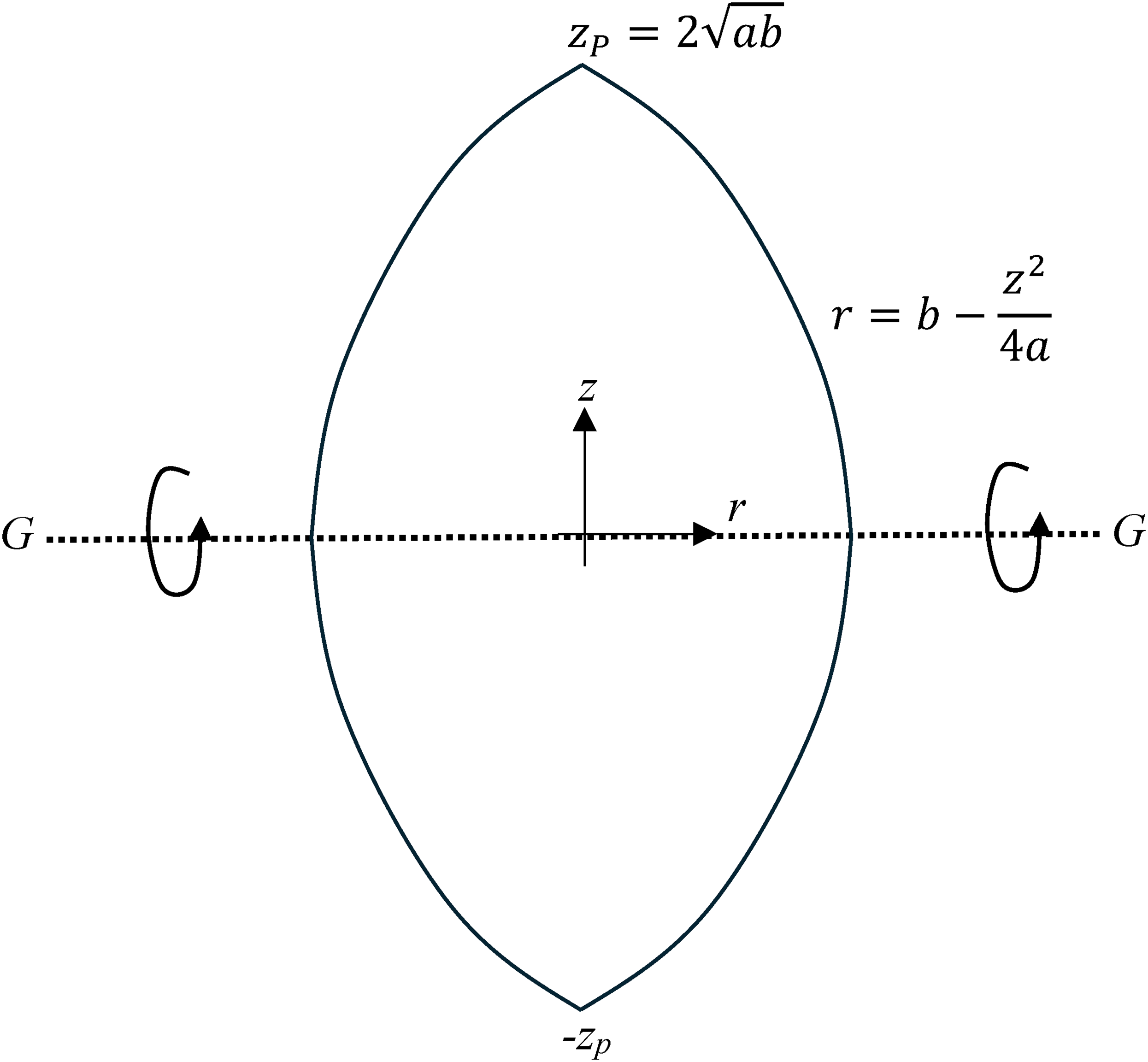
Schematic of an American football.

Where z_cp is the center of pressure. Observation of the flight of a well thrown American football, tells us that the ball does not rotate backwards about its center of mass Alam et al.^21,22 presented an analysis of the aerodynamics of an American football in flight, explaining this counter intuitive behavior. The details of the analysis, can be found in,^21,22 in summary it is due to how the projected area in the horizontal direction and vertical direction of the American football changes during flight.

The parameters defining an American football are given in.⁴ The American football is taken to be an axisymmetric shell, with a parabolic profile,

r = b - \frac{z^{2}}{4 a}

z_{P} = 2 \sqrt{a b}

(34)

Where $\pm z_{P}$ denotes the apexes of the American football, see Figure 13. The dimensions of an American football are b = 0.086 m, z_P = 0.141 m and m = 0.411 kg. The mass moment of inertia for an American football, determined using 1^st principles and Mathematica is I_GG,Af = 0.002829 kgm².⁴

The Monte-Carlo methods, No PAT method and PAT method are applied to the American football by representing it as a composite of truncated conical shells, and two conical shells at the apexes of the ball. After some numerical experimentation, an appropriate number of axisymmetric components is N_tc=200. The Error_RMS vs. N_fun for the two Monte-Carlo methods, No PAT method and PAT method, are shown in Figure 14. Figure 14, shows that the PAT method is marginally superior to the No PAT method. The number of function evaluations to achieve an error, Error_RMS=0.1%, for the No PAT method, and PAT method is N_fun,0.1%=104,000 and N_fun,0.1%=81,300 respectively, the speed-up is S_P = 1.28. These results are consistent with the performance of the two Monte-Carlo methods, applied to a spherical shell. The Error_RMS curve labelled “AF curve (38)” in Figure 14 is discussed below.

Figure 14.

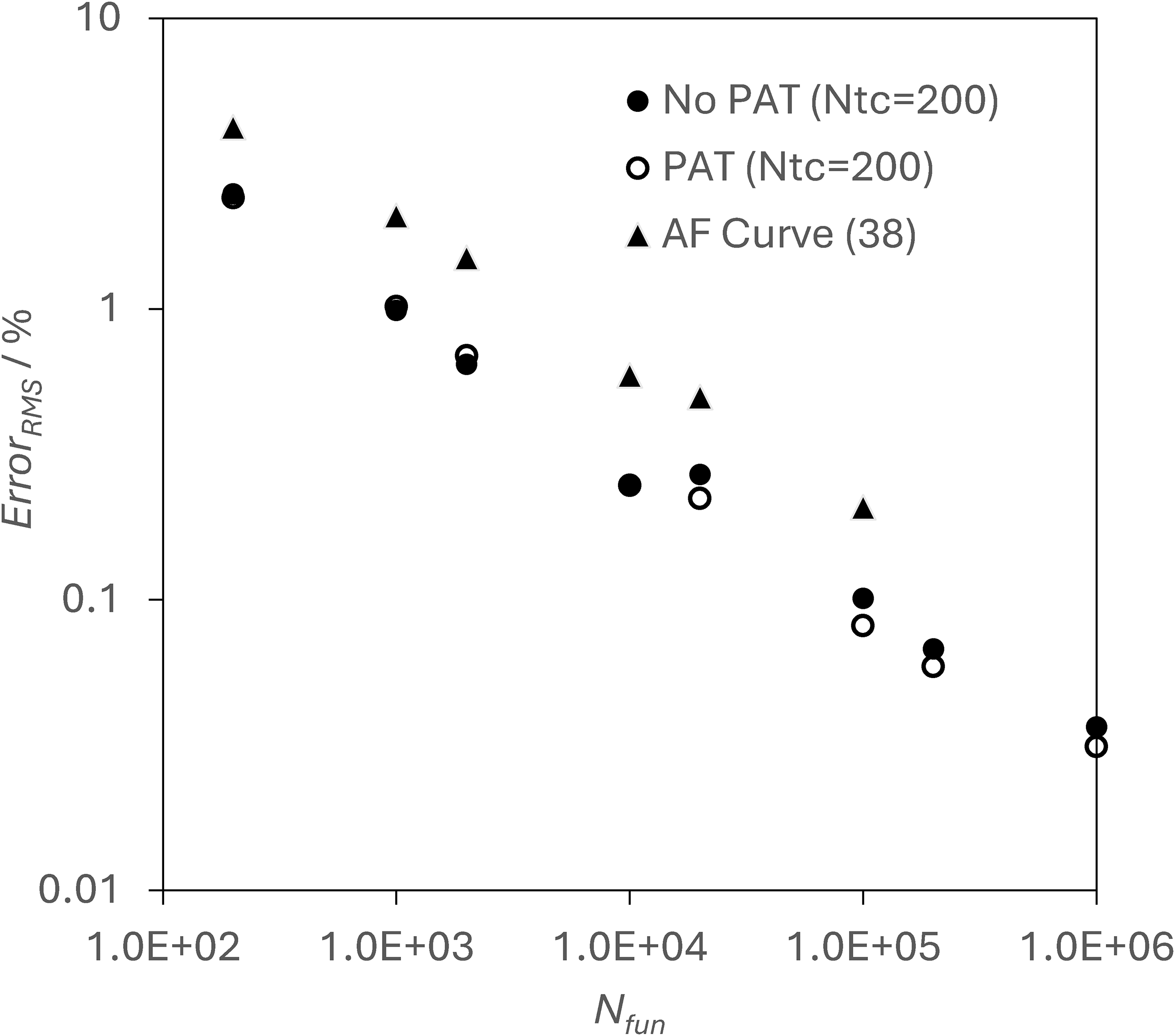
Error_RMS vs. N_fun, for the MMoI of an American football calculated using the No PAT method, the PAT method and the Ra_z vs z_i curve fit (38).

It is interesting to compare the performance of the Monte-Carlo methods, applied to the American football example, where the analytical curve of the surface profile (34), is used verses when the shape is represented as a composite of truncated conical shells. For the Monte-Carlo method based on (34), the mapping for the z coordinate to the pseudo-random number, Ra_z is given implicitly as,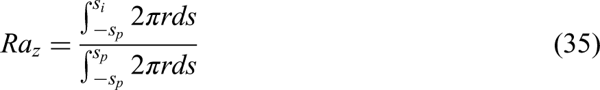

R a_{z} = \frac{\int_{- s_{p}}^{s_{i}} 2 π r d s}{\int_{- s_{p}}^{s_{p}} 2 π r d s}

(35)

The differential element, ds and the integration bounds relate to the coordinate, s defined to be the coordinate along the curvature of the American football. The integration is changed to be in the direction of the z coordinate direction.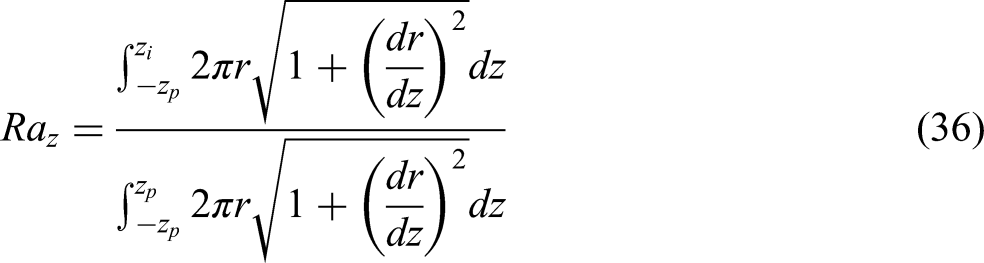

R a_{z} = \frac{\int_{- z_{p}}^{z_{i}} 2 π r \sqrt{1 + {(\frac{d r}{d z})}^{2}} d z}{\int_{- z_{p}}^{z_{p}} 2 π r \sqrt{1 + {(\frac{d r}{d z})}^{2}} d z}

(36)

Using (34) to substitute for r and 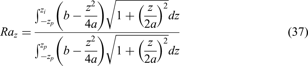$\frac{d r}{d z}$ , and removing the common factor 2π gives,

R a_{z} = \frac{\int_{- z_{p}}^{z_{i}} (b - \frac{z^{2}}{4 a}) \sqrt{1 + {(\frac{z}{2 a})}^{2}} d z}{\int_{- z_{p}}^{z_{p}} (b - \frac{z^{2}}{4 a}) \sqrt{1 + {(\frac{z}{2 a})}^{2}} d z}

(37)

To take the analysis further, requires evaluating the two integrals in (37), and then rearranging the equation such that the subject of the equation is z_i. This is not easily accomplished, an alternative route is to evaluate the integrals numerically, and then to calculate a composite curve fit to the equation defined implicitly by (37),

z_{i} = f_{c f} (R a_{z})

(38)

The functional relationship between Ra_z and z_i is shown in Figure 15. Due to the symmetry about the axis of rotation G-G, of an American football see Figure 13, it is sufficient to provide a curve fit for (37) for $0 \leq R a_{z} \leq 0.5$ . For pseudo-random numbers above 0.5 the transformations,

R a_{z} \to 1 - R a_{z}

z_{i} \to - z_{i}

(39)

reproduce the curve shown in Figure 15. The curve in Figure 15 is almost linear for a large interval of Ra_z, in the middle of the unit interval. A piecewise composite fit is calculated using polynomials of order one, two, three or four for different intervals of Ra_z space. For the curve fit prescribed the correlation coefficient is above 0.999. The accuracy of the Monte-Carlo method is sensitive to the accuracy of the curve fit (38).

Figure 15.

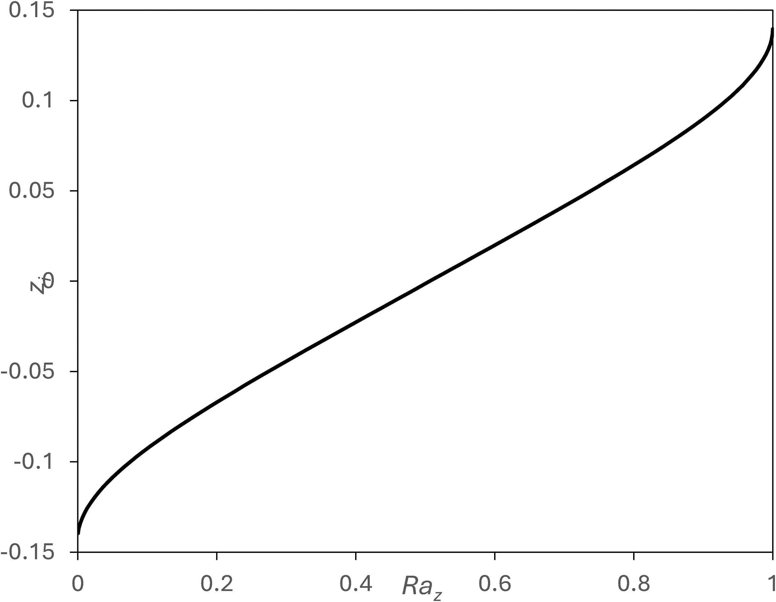
The mapping from the pseudo-random number Ra_z to the axial coordinate, z_i of an American football.

Figure 14 shows the Monte-Carlo method Error_RMS curve using the curve fit (38), labelled as AF curve (38). Error_RMS is only calculated for $200 \leq N_{f u n} \leq 100, 000$ . To achieve a more accurate estimate of the mass moment of inertia of the American football, requires a more accurate curve fit (38). From Figure 14, it is clear that the Monte-Carlo methods based on the composite truncated conical shells, are more accurate than one based on the analytical curve (34). The number of functions to achieve an error of Error_RMS=0.1%, for the AF curve (38) is N_fun=467,000. For completeness this is included in Table 1. Note to achieve this would require a more accurate Ra_z- z_i mapping. The reason for the better accuracy of the composite truncated conical shell representation of the American football is due to two issues; the small errors in the representation (38) of the Ra_z- z_i mapping, but what is probably more important is that the composite representation ensures a more even distribution of points within the American football surface. This is similar to stratified sampling where the strata are the individual truncated conical shells.²³

Conclusion

In this paper, the mass moment of inertia for a truncated conical shell is formulated. The mass moment of inertia, of a number of axisymmetric shells and axisymmetric 2-dimensional shapes are shown to be limiting cases of a truncated conical shell. Two variants of the Monte-Carlo method for evaluating the MMoI, for a truncated conical shell are considered, the No PAT method, and the PAT method. For the No PAT method, the MMoI for an axis through the base, parallel to the base, I_BB is evaluated directly. For the PAT method the Monte-Carlo method is used to evaluate the MMoI about the center of mass parallel to the base, I_GG, and then the parallel axis theorem (2) is used to evaluate I_BB.

The two Monte-Carlo methods are applied to the calculation of the MMoI for a number of different axisymmetric shells, and axisymmetric 2-dimensional shapes. In general, provided the center of mass of the shape is non-zero, the PAT method tends to be more efficient than the No PAT method. The conclusion here concerning Monte-Carlo method efficiency, is similar to² except the speed-up of the PAT method does not tend to be as large for axisymmetric shells compared to axisymmetric solid shapes. For example, the speed-up for a solid rod, the shape closest to a narrow tube is S_P = 21.7.² The speed-up achieved for a narrow tube, using the PAT method relative to the No PAT method is S_P =13.4.

This paper, and the linked paper² make it possible for the mass moment of inertia for any axisymmetric body, to be modelled as a composite of axisymmetric shells, and solid shapes. The final part of this paper is the application of the analysis, to possible student projects using the Monte-Carlo method, to evaluate the MMoI of shapes of interest to students, taking a course on rotational dynamics.

Footnotes

Nomenclature

ORCID iD

Peter S. Cumber

Funding

The author received no financial support for the research, authorship, and/or publication of this article.

Declaration of conflicting interests

The author declared no potential conflicts of interest with respect to the research, authorship, and/or publication of this article.

Data availability statement

Data sharing not applicable to this article as no datasets were generated or analyzed during the current study.

Appendix A1. Derivation of the mass moment of inertia for a truncated conical shell.

The mass moment of inertia for a truncated conical shell, can be derived using first principles, and the parallel axis theorem.

The starting point is the schematic diagram shown in Figure A1. The mass moment of inertia for a hoop, defined in Figure A1 about the axis of rotation x-x is, (\rm A1)

d I_{x x} = \frac{1}{2} r^{2} d m

Applying the parallel axis theorem,

d I_{B B, t c} = (\frac{1}{2} r^{2} + z^{2}) d m = (\frac{1}{2} r^{2} + z^{2}) r d z 2 ρ π d r

d r = \frac{Δ}{\cos θ} = Δ \frac{S_{t c}}{H_{t c}} = Δ \frac{\sqrt{H_{t c}^{2} + {(R_{b} - R_{t})}^{2}}}{H_{t c}}

Where Δ is the thickness of the truncated conical shell, and S_tc is defined in Figure A1. (\rm A2)

d I_{B B, t c} = (\frac{1}{2} r^{2} + z^{2}) r d z 2 ρ π Δ \frac{\sqrt{H_{t c}^{2} + {(R_{b} - R_{t})}^{2}}}{H_{t c}}

Integrating between z = 0 and z = H_tc. (\rm A3)

I_{B B, t c} = \int_{0}^{H_{t c}} (r^{2} + z^{2}) r d z 2 ρ π Δ \frac{\sqrt{H_{t c}^{2} + {(R_{b} - R_{t})}^{2}}}{H_{t c}}

The equation of the line defining the curved surface of the truncated conical shape is,

r = R_{b} - z \frac{Δ R}{H_{t c}}

where

Δ R = R_{b} - R_{t}

Substituting for r as a function of z in (A3) and integrating gives (\rm A5)

I_{B B, t c} = (\frac{1}{2} R_{b}^{3} - \frac{3}{4} R_{b}^{2} Δ R + \frac{1}{2} R_{b} {(Δ R)}^{2} - \frac{1}{8} {(Δ R)}^{3} + (\frac{1}{3} R_{b} - \frac{1}{4} Δ R) H_{t c}^{2}) 2 ρ π \sqrt{H_{t c}^{2} + {(Δ R)}^{2}} Δ

Introducing the mass, m of the truncated conical shell gives the result.

m = ρ π (R_{b} + R_{t}) \sqrt{H_{t c}^{2} + {(Δ R)}^{2}} Δ

I_{B B, t c} = m [{\frac{R_{b}^{3} - \frac{3}{2} R_{b}^{2} Δ R + R_{b} {(Δ R)}^{2} - \frac{1}{4} {(Δ R)}^{3}}{R_{b} + R_{t}}} + H_{t c}^{2} {\frac{\frac{2}{3} R_{b} - \frac{1}{2} Δ R}{R_{b} + R_{t}}}]

Which can be simplified to, (\rm A6)

I_{B B, t c} = m [\frac{1}{4} (R_{b}^{2} + R_{t}^{2}) + \frac{1}{6} H_{t c}^{2} {\frac{R_{b} + 3 R_{t}}{R_{b} + R_{t}}}]

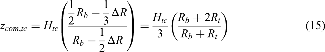
The center of mass for a truncated conical shell is, (\rm A8)

z_{c o m, t c} = H_{t c} (\frac{\frac{1}{2} R_{b} - \frac{1}{3} Δ R}{R_{b} - \frac{1}{2} Δ R})

The derivation of z_com,tc, is left as an exercise. The mass moment of inertia parallel to B-B, and through the center of mass is, (\rm A9)

I_{G G, t c} = m [\frac{1}{4} (R_{b}^{2} + R_{t}^{2}) + \frac{1}{6} H_{t c}^{2} {\frac{R_{b} + 3 R_{t}}{R_{b} + R_{t}}}] - m z_{c o m, t c}^{2}

References

Meriam

Kraige

Bolton

. Engineering Mechanics Dynamics, 8^th Edn. USA: John Wiley & Son Inc., 2016.

Cumber

. Mass moments of inertia for axisymmetric shapes evaluated using the Monte-Carlo method – Truncated cones, in preparation.

Technical Information Summary Apollo-10 (AS-505). NASA. 1969.

Horn

Fearn

. On the Flight of the American Football, arXiv:0706.0366v1, 2008, 1–22.

Cumber

. Truncated cone – A universal primitive shape for axisymmetric view factor systems”. ASME Journal of Heat and Mass Transfer 2024; 146: 034501–1.

Pope

. A monte-carlo method for the PDF equations of turbulent reactive flow. Combust Sci Technol 1981; 25: 159–174.

Pope

. Assessment of numerical accuracy of PDF/monte carlo methods for turbulent reactive flows. J Comp Phys 1999; 152: 192–230.

Mustata

Valino

Jimenez

, et al. A probability density function eulerian monte carlo field method for large eddy simulations: Application to a turbulent piloted methane/air diffusion flame (sandia D). Combust Flame 2006; 145: 88–104.

Todorov

. Computing high dimensional integrals with monte carlo methods. Journal of Scientific and Applied Research 2016; 10: 1–16.

10.

Ritter

. Monte carlo integration – a case study for simulation. International Journal Mathematical Education in Science and Technology 2014; 45: 131–145.

11.

Montgomery

Runger

. Applied Statistics and Probability for Engineers. 6th Ed. New York: Wiley, 2014.

12.

Lapeyre

Pardoux

Sentis

. Introduction to Monte-Carlo Methods for Transport and Diffusion Equations. Oxford, UK: Oxford University Press, 2003.

13.

Ochiai

. Numerical integration to obtain moment of inertia of homogeneous material. Eng Anal Boundary Elem 2019; 101: 149–155.

14.

Bissell

Ritchey

Stevens

. Measuring the moment of inertia of a rigid body using a swing-pendulum. Phys Educ 2023; 58: 065022.

15.

Chen

Wang

Hao

, et al. Measurement of moment of inertia of objects based on the law of conservation of angular momentum. Theoretical and Natural Science 2025; 87: 218–226.

16.

Podhorodeski

Sobejko

. A project in the determination of the moment of inertia. Int J Mech Eng Educ 2005; 33: 319–338.

17.

Hunt

Lipsman

Rosenberg

. A Guide to MATLAB: For Beginners and Experienced Users, 2014, Cambridge University Press, 2014.

18.

Cumber

. Mass moment of inertia evaluation using the Monte-Carlo method and the parallel axis theorem. Int J Math Educ Sci Technol 2026: 1–22. https://doi.org/10.1080/0020739X.2026.2664768

19.

Apollo/Saturn V Postflight Trajectory AS-505, Boeing Company Aerospace Group Southeast Division, 1969, NASA.

20.

SIVB-503N Stage Flight Test Plan, McDonnell Douglas Astronautics Company, (1968), NASA.

21.

Alam

Chowdhury

Moria

, et al. A comparative study of football aerodynamics. Procedia Eng 2010; 2: 2443–2448.

22.

Alam

Smith

Chowdhury

, et al. Aerodynamic drag measurement of American footballs. Procedia Eng 2012; 34: 98–103.

23.

Kish

. Survey Sampling. New York: John Wiley & Sons, Inc., 1965.

Mass moments of inertia for axisymmetric shells evaluated using the Monte-Carlo method – Truncated conical shells

Abstract

Keywords

Introduction

Monte-Carlo method

Monte-Carlo method applied to the MMoI of a truncated conical shell

Approximating the MMoI for other axisymmetric shells

Conical shell specification

Tube specification

2-Dimensional disc

2-Dimensional Annulus

Hemispherical shell and spherical shell

Application of the Monte-Carlo method to calculating MMoI

Truncated conical shell

Tube

Hemispherical shell

Conical shell, spherical shell, disc and annulus

Examples of student projects for the calculation of MMoI of axisymmetric bodies

Estimating the MMoI of a Saturn V rocket (Apollo 10)

Calculating the MMoI of an American football

Conclusion

Footnotes

Nomenclature

ORCID iD

Funding

Declaration of conflicting interests

Data availability statement

Appendix A1. Derivation of the mass moment of inertia for a truncated conical shell.

References