Calculating Probability in Sex Offender Risk Assessment

Abstract

Risk is the probability of an adverse event or outcome. In a previous article, I compared the Bayesian and Frequentist models of defining probability. This article compares the Bayesian and regression models of quantifying probability. Both approaches are widely used in the biomedical and behavioral sciences even though they yield different results. No consensus has emerged as to which is more appropriate. The choice between them remains controversial. This article concludes that the Bayesian model provides a viable alternative to logistic regression and may be more useful in quantifying the absolute recidivism risk of individual sex offenders. It shows how evaluators can easily calculate Bayesian probabilities and their associated credible intervals from an actuarial data set. Last, the article proposes a forensic practice guideline that evaluators do not conclude that an offender meets an absolute risk threshold unless the subject’s risk exceeds the threshold by a credible margin of error.

Keywords

risk assessment probability sexual recidivism prediction

Introduction

Predicting individuals’ risk of recidivism is important for treatment, supervision, and public safety. It is critical in the United States, where courts use absolute risk predictions to determine whether sex offenders should be committed as sexually violent persons (SVPs). Risk is the probability of an adverse event or outcome. Probability can be defined in either Frequentist or Bayesian terms (Elwood, 2016). Frequentist probability is defined by the relative frequency of an event, how frequently an event occurs over a series of repeated trials. However, a single trial has no relative frequency. Therefore, Frequentist probability cannot be meaningfully applied to a single case. Bayesian probability is not defined by relative frequency but by our knowledge about an outcome. It can be applied to single events like sexual recidivism.

This article compares models of calculating absolute risk. There are basically two statistical models that are used to predict risk (Pepe et al., 2007). The first quantifies risk as a function of a predictor, typically using logistic or Cox regression. The second quantifies risk by binary classifications that yield predictive powers based on Bayes’s theorem. Both models are widely used but yield different results. No consensus has yet emerged as to which is the most appropriate or under what circumstances. The choice between them remains controversial. That controversy extends to sex offender risk assessment because evaluators use actuarial scales like the Static-99R (Harris, Phenix, & Williams, 2009) and Violence Risk Scale–Sexual Offender Version (VRS-SO; Olver, Beggs-Christofferson, Grace, & Wong, 2014) to predict risk from the recidivism rates found in longitudinal cohort studies of sex offenders. Because Bayesian probability is not widely used in sex offender risk assessment, I show how evaluators can calculate Bayesian probabilities and their margins of error from any data set by using freely available online calculators.

This article looks beyond the sex offender assessment literature to biostatistics and epidemiology, both of which have developed statistical models to predict the risk and causes of health-related conditions. Hanson and Howard (2010) contended that comparing the risk of sexual recidivism with the risk of medical conditions is inappropriate. They argued that risk assessment predicts a future event and thus is prognostic, whereas medical assessment predicts a current condition and thus is diagnostic. However, Pepe (2003) noted that “prognosis can be considered as a special type of diagnosis, where the condition to be detected is not disease, per se, but is a clinical outcome of interest” (p. 1). Moreover, scales like the Framingham Risk Scale (Framingham Heart Study, 2013) and the Breast Cancer Risk Assessment Tool (BCRAT; Gail et al., 1989) are prognostic. They are often used in medical practice to predict the lifetime risk of individual patients to contract specific diseases. Methods of predicting disease apply equally to predicting the risk of any binary outcome, including sexual recidivism.

Risk Prediction Models

Logistic Regression

Logistic regression describes the association between one or more independent variables and a categorical (e.g., low, medium, or high) dependent variable. When the dependent variable has only two categories (e.g., yes/no), it is termed binary logistic regression. Logistic regression has two advantages in relating a scale score to the probability of a binary outcome. Like any regression method, it provides smooth predictions of an outcome across the values of a predictor. Logistic regression is better suited for predicting binary outcomes because, unlike ordinary linear regression, it constrains the predicted probabilities between 0% and 100%. Logistic regression is widely used throughout the biomedical and behavioral sciences to predict the risk of binary outcomes. Actuarial scales like the Static-99R (Phenix, Helmus, & Hanson, 2012, 2015) and VRS-SO (Olver et al., 2014) use logistic regression to predict the probability of a single binary outcome (sexual recidivism) from the level of a single predictor variable (score).

Predictive Power

Predictive powers are derived from binary classifications of test results (like Static-99R scores) and outcomes (like sexual recidivism). Positive test results (+ test) are those at or above a specified cutoff. Negative test results (− test) are those below the cutoff. Likewise, the outcome is either positive if it occurred or negative if it did not. If scores on a scale are used to specify the cutoff, each score will yield different numbers of positive and negative tests and positive and negative outcomes. Positive predictive power (PPP; also known as positive predictive value [PPV]) is the probability that a subject with a positive test result will have the outcome. It is the proportion of test positives that have the outcome. Negative predictive value (NPP) is the inverse, the probability that a subject with a negative test result will not have outcome. It is the proportion of negatives that do not have the outcome. Pepe (2003) contended that “predictive values are not used to quantify the inherent accuracy of the test. Rather, predictive values quantify the clinical value of the test” (p. 16). PPP is more important than negative predictive power in forensic cases because the critical question is whether an individual’s risk exceeds a specified threshold. Predictive powers have been presented for the Static-99 (Beauregard & Mieczkowski, 2009; Bengtson & Långström, 2008; Wollert, 2006), the Static-99R (Campbell, 2011; Eher, Olver, Heurix, Schilling, & Rettenberger, 2015), and the VRS-SO (Eher et al., 2015). Still, Bayesian predictive powers have not been widely adopted in sex offender risk assessment.

Discussion

Pepe, Janes, Longton, Leisenring, and Newcomb (2004) showed that even a strong association between a predictor and an outcome does not imply that the predictor can discriminate individuals who will have the outcome. Pepe and her colleagues (2007) argued that although logistic regression is adequate in etiologic research, it does not address the ability of a test to correctly classify individuals or predict risk in a population. A working group of the international Cochrane Collaboration of health care researchers and professionals (Bossuyt et al., 2013) concluded that paired summary statistics like PPPs and NPPs are clinically more useful than global statistics because they distinguish false positives and false negatives. Parikh, Mathai, Parikh, Sekhar, and Thomas (2008) recommended that physicians routinely use PPPs and NPPs in their practice because they clearly show the advantages and limitations of the clinical tests they use to make medical decisions. Pepe (2003) proposed that predictive powers quantify the clinical utility of a biomedical marker because clinicians want to know the probability that their patient has or will have a disease given a test result.

Barbini and his colleagues (2007) compared eight models to predict the incidence of morbidity following cardiac surgery. They concluded that Bayesian models offered a good compromise between complexity and predictive performance. They noted that Bayesian models can more easily be updated with new information than logistic regression models. Singh (2013) argued that PPPs and NPPs contribute to sex offender risk assessment by emphasizing the prospective prediction of sexual recidivism. In SVP cases, courts want to know the probability that an offender will commit another sex offense given his Static-99R score and other risk factors. There is clearly a broad consensus that the Bayesian model of probability offers advantages to logistic regression in predicting risk, including the recidivism risk of sex offenders.

Calculating Predictive Power

Bayesian probabilities are based on Bayes’s theorem. Applications of Bayes’s theorem can be (and often are) complicated, but for our purpose, Bayes’s theorem is simply the mathematical expression for the inverse of a conditional probability. A conditional probability depends on (is conditional on) the value of another probability. Prior probabilities (or “priors”) reflect the information we start with, the overall population baserate of an outcome. Posterior probabilities reflect additional information, such as a test result. Per Bayes’s theorem,

p (\frac{A}{B}) = p (\frac{B}{A}) \times \frac{p (A)}{p (B)} .

$p (A / B)$ is the posterior probability, the probability of A given B. It is called the positive predictive power. $p (B / A)$ is the inverse of the $p (A / B)$ the probability of B given A. $p (A)$ is the probability of A, and $p (B)$ is the prior probability of B. It may be helpful to think of prior and posterior probabilities as pretest and posttest probabilities.

All this might seem very arcane to evaluators until we set A = sexual recidivism and B = a positive (+) Static-99R result. By Bayes’s theorem,

p (Recidivism | + Static - 99 R) = p (+ Static - 99 R | recidivism) \times \frac{Recidivism baserate}{p (+ Static - 99 R)},

which is precisely what forensic evaluators seek and why they use actuarial scales.

Suppose an evaluator scores a high-risk offender 6 on the Static-99R. Static-99R scores of 6 and above are test positives. Scores of 5 and below are test negatives. From the detailed Static-99R 10-year High-Risk Need (HR/N) recidivism rate table (A. Harris, Phenix, & Williams, 2009; see Table 1), the sums of recidivists and nonrecidivists with scores at or above 6 and 5 and below are shown in the Σ columns. The positive outcome is recidivism; the negative outcome is nonrecidivism. Two hundred four out of 703 HR/N samples at 10 years recidivated. Thus, the recidivism base ate is 204 / 703 = 29.0%. Two hundred three (85 + 118) of the offenders had a +Static-99R score (≥6). Thus, 203 / 703, or 28.9% of the HR/N offenders had a +Static-99R score. Of the 204 offenders who recidivated, 85 had a +Static-99R score. Thus, $p (+ Static - 99 R | recidivism) = 85 / 204$ , or 41.7%. By Bayes’s theorem, the $P P P = . 417 \times (. 290 / . 289) = . 419 or 41.9 %$ .

Table 1.

Static-99R 10-Year High Risk/Need Observed Sexual Recidivism Rates.

Score	Σ	Recidivists	Nonrecidivists	Σ
−2	119	0	2	381
−1		2	22
0		3	28
1		5	51
2		14	28
3		22	60
4		34	96
5		39	94
6	85	32	51	118
7		29	36
8		12	17
9		8	9
10		4	5
11		0	1
Total		204	499

Source. Harris, Phenix, and Williams (2009).

Bayes’s theorem helps us avoid two common errors in applying probabilities. First, people often confuse a conditional probability with its inverse, assuming that $p (A / B) = p (B / A)$ The fact that most people with lung cancer were heavy smokers does not mean that most heavy smokers develop lung cancer. Second, Bayes’s theorem shows that the probability of an outcome depends on its baserate, its population incidence. Even highly accurate tests may not predict rare (low baserate) disorders well enough to be useful (Elwood, 1993a, 1993b). Of course, the converse is also true; even moderately predictive tests can do well at predicting common (high baserate) outcomes.

Freeman and Mossman (2009) took the view that “all forensic methods are really tests and all forensic opinions are really test results” (p. 695). This article thus considers actuarial scales like the Static-99R and VRS-SO to be tests. Test results can be represented by true positives and false positives. Knowing the frequencies, we can easily construct a 2 × 2 binary classification table for each score of an actuarial score. Classification tables are useful for two reasons. First, probabilities are much easier to visualize when the information is given in frequencies rather than probabilities. Second, classification tables enable us to easily calculate predictive values, sensitivity, and specificity. Evaluators can also use the frequencies easily obtain the AUC (area under the curve) by an online calculator (e.g., Eng, 2015). Kanchanaraksa (2008) provided a graphic tutorial on binary classifications, predictive powers, sensitivity, and specificity. Glaros and Kline (1988) discussed them in more detail.

The classification table for a Static-99R score of 6 from the previous example is shown in Table 2. The columns (+, −) denote positive or negative outcomes. The rows (+, −) denote positive or negative Static-99R scores. Offenders with a positive test result who recidivated are true positives; those with a positive test result who did not recidivate are false positives. Likewise, offenders with a negatives test result who did not recidivate are true negatives; those with a negative test result who did recidivate are false negatives.

Table 2.

Binary Classification Table.

		recidivism
		+	−
Static-99R ≥ 6	+	85	118	203
Static-99R < 6	−	119	381	500
		204	499	703

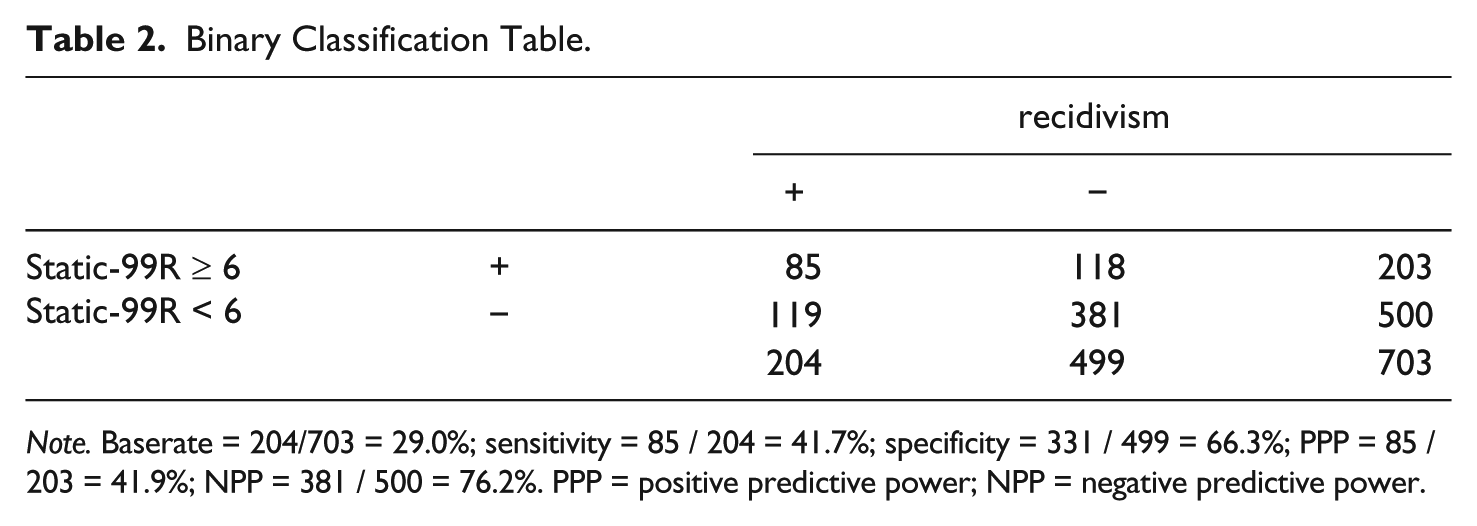
Note. Baserate = 204/703 = 29.0%; sensitivity = 85 / 204 = 41.7%; specificity = 331 / 499 = 66.3%; PPP = 85 / 203 = 41.9%; NPP = 381 / 500 = 76.2%. PPP = positive predictive power; NPP = negative predictive power.

The predictive powers are calculated by rows. The PPP for an HR/N Static-99R score of 6 is the ratio of true positives to all test positives, or 85 / 202 = 41.9%, which is exactly what we found using the formula for Bayes’s theorem. The NPP, the posterior probability of nonrecidivism given a negative Static-99R score, is 381 / 500 = 76.2%. The sensitivity and specificity are calculated by columns: sensitivity = 41.7% and specificity = 66.3%. I calculated an AUC of .64 for the 2009 HR/N group using a popular online ROC analysis program (Eng, 2015). The lower AUC is precisely what Helmus, Thornton, Hanson, and Babchishin (2012) predicted when the sample is restricted to high-risk offenders. Evaluators can use 2 × 2 tables in the same way to calculate PPP for score on the Static-99R, VRS-SO, or other scale.

The Debate in Sex Offender Risk Assessment

A leading figure in SVP assessment posted to a professional forum that “all the talk of false positives etc. assumes that the task is prophecy whereas SVP laws actually require risk assessment.”(Anonymous) Actually, the task of SVP risk assessment is prophecy. Prophecy is prediction. Prediction is simply inferring the value of some unknown data from some known data (Kruschke, 2011). Thus, risk assessment, prediction, and prophecy are the same.

A colleague recently criticized using PPPs for the Static-99R because they are dependent on the outcome baserate, and thus, PPPs are not a property of the scale itself. However, calibration, how well a test predicts an outcome, is the joint property of the test and the sample to which it is applied, whether one uses PPP or logistic regression. For example, the BCRAT (Gail et al., 1989) was calibrated in studies of White American women. It had to be recalibrated to predict the risk of women in Asia, where the incidence of breast cancer is much lower (Matsuno et al., 2011). Dependence on baserate is a strength of the PPP, not a weakness. Moreover, recidivism rates predicted by logistic regression are also sensitive to baserate (Sharma, McGee, & Kibria, 2011). An advantage of PPPs is that they can easily be revised to accommodate different outcome baserates, using either Bayes’s theorem or binary tables.

G. T. Harris and Rice (2007) favored selection ratios based on the AUC rather than PPPs to base optimal risk decisions by the relative costs of decision errors. However, SVP risk thresholds are defined by statute (e.g., “likely” or “more likely than not”), not by cost/benefit ratios. Moreover, the AUC and PPP are fundamentally different concepts. AUCs predict test results like Static-99R scores, not outcomes like sexual recidivism. They portray the trade-off between false positives and negatives. AUCs do not reflect predictive accuracy (e.g., Singh, 2013; Vickers & Cronin, 2010). They measure how well a scale discriminates an outcome across a range of scores while the PPP predicts the outcome for each score.

Critics of binary classifications in sex offender risk assessment routinely cite AUCs to support the validity of actuarial scales like the Static-99/R. However, AUCs are plots of likelihood ratios (sensitivity / 1 − specificity), which are derived from binary classifications of “false positives etc.” One cannot coherently accept AUCs while rejecting the classifications on which they are based.

Margin of Error

Pepe (2003) proposed that “before a test can be recommended for use in practice, its diagnostic accuracy must be rigorously assessed” (p. 3). The Standards for Educational and Psychological Testing (American Educational Research Association, 1999) proposes that evaluators report the reliability and standard error of any score they interpret. The Specialty Guidelines for Forensic Psychologists (American Psychological Association, 2011) calls for forensic evaluators to identify limitations of their tests, which presumably includes their margins of error. Senior reviewers for the American Board of Forensic Psychology (Grisso, 2010) advise evaluators to “describe any important ways in which one’s data or interpretations leave room for error or alternative interpretations” (p. 109). The error rate of a scientific method is among the four Daubert criteria for the admissibility of expert testimony (Daubert v. Merrell Dow, 1993). One jurist (Jabbar, 2010) argued that the error rate is primary and that trial judges should not even consider other Daubert validity factors unless an error rate is not available. R. J. Wilson and Looman (2010) defended their qualifying risk statements within a margin of error simply “because it is the truth and this reality needs to be acknowledged” (p. 312). Given the modest AUCs for the Static-99R (e.g., Helmus et al., 2012), risk predictions from the Static-99R have substantial margins of error. Clearly, incorporating margin of error in risk assessments is supported by accepted practice guidelines, expert advice, and judicial opinions.

Calculating Bayesian Credible Intervals

As there are Frequentist and Bayesian concepts of probability, there are Frequentist and Bayesian concepts of margin of error. Much of the debate over margin of error in sex offender assessment comes from the failure to distinguish Bayesian credible intervals from Frequentist confidence intervals (CIs). Like Frequentist probabilities, Frequentist CIs apply to repeated trials, not single events. By contrast, Bayesian credible intervals, like Bayesian probabilities, can be applied to single events (Oleson, 2010) like sexual recidivism.

Frequentists estimate a true, fixed population mean and calculate an interval based on the sample distribution. By definition, the true mean has a fixed value, not a distribution, so Frequentists cannot claim a 95% probability that the interval contains the true mean. They can only say something like “95% of similar intervals would contain the true mean, if each interval were constructed from a different random sample like this one” (Annis, 2013). Annis (2013) continued, “now the Bayesian can say what the frequentist cannot: ‘there is a 95% probability that this interval contains the mean.’”

Morey, Hoekstra, Rouder, Lee, and Wagenmakers (2016) compared four CI procedures with Bayesian credible intervals. They concluded that only the Bayesian interval properly reflected precision and plausibility. Scurich and John (2011) argued, “it is simply unintelligible to employ frequentist confidence intervals to describe the precision of actuarial risk estimates . . . Bayesian credible intervals are necessary—in principle—to describe probabilistically the precision of actuarial risk estimates . . .” (p. 242).

Although PPPs can be easily calculated from a 2 × 2 binary table, calculating Bayesian credible intervals is more complicated. Fortunately, user friendly calculators are freely available online. Douglas Mossman, a forensic psychiatrist, and James Berger, a statistician (Mossman & Berger, 2001), addressed the common task in medicine of predicting a patient’s risk of a disorder given a laboratory test result. They used a Monte Carlo procedure to calculate 95% two-tailed Bayesian intervals for PPPs and found the intervals performed better than four other interval methods they evaluated. Mossman and Berger claimed their algorithm could be run on common spreadsheet programs, though I doubt many evaluators would undertake that task on their own.

John Crawford, a neuropsychologist, and his colleagues at the University of Aberdeen in Scotland, addressed a problem similar to that faced by forensic evaluators: comparing an individual patient’s test score with a normative sample, especially when the normative sample is small. Crawford, Garthwaite, and Betkowska (2009a) extended Mossman and Berger’s method and devised a computer program that evaluators can download or use online to obtain PPP and NPP values and both one- and two-tailed 95% credible intervals (Crawford, Garthwaite, & Betkowska, 2009b).

Table 3 lists the PPPs for the 2009 Static-99R HR/N group along with their one-tailed 90% and 95% Bayesian credible intervals (Crawford et al., 2009b). The PPP values are identical to those of Campbell (2011). Eher et al. (2015) found a lower PPP for a Static-99R of 4 (28.6% vs. 33.9%), which is expected given their lower recidivism baserate (8.3% vs. 29% for the Static-99R HR/N group). The intervals around the 2009 Static-99R HR/N PPPs in Table 3 were calculated from 100,000 Monte Carlo trials (which illustrates why Bayesian probability became practical only after the advent of powerful desktop computers). Other free online calculators (Hutchon, 2015; MedCalc Software, 2016; Schwartz, 2010) yield virtually identical results for all but extreme scores.

Table 3.

10-Year Sex Offense Charges: PPPs^a for the 2009 Static-99R HR/N group^b.

Cutoff score	Test+	True+	Test−	True−	PPP	One-tail lower limit^a
Cutoff score	Test+	True+	Test−	True−	PPP	95%	90%
−1	701	204	2	2	291	262	267
0	677	202	26	24	298	270	275
1	646	199	57	52	308	279	284
2	590	194	113	103	329	298	303
3	548	180	155	131	329	296	301
4	466	158	237	191	339	303	309
5	336	124	367	287	369	326	333
6	203	85	500	381	419	363	372
7	120	53	583	432	442	367	379
8	59	24	644	464	407	304	321
9	27	12	676	484	444	292	317
10	10	4	693	493	400	169	207
11	1	0	702	498	332	002	056

Note. PPP = positive predictive power; HR/N = high-risk need.

Crawford, Garthwaite, and Betkowska (2009b).

Harris, Phenix, and Williams (2009).

The bold-faced values are probabilites based on observed rates.

Evaluators can use Table 3 in the same way they use the Static-99R logistic regression rate tables (Phenix et al., 2012, 2015). Of course, evaluators can devise their own recidivism rate table using their own data and assumptions. Readers familiar with the Static-99R will note that the PPPs are higher than the logistic regression rates (Elwood, Kelley, & Mundt, 2016; Phenix et al., 2012) at low Static-99R scores and lower than the logistic regression rates at high scores. Also, the PPPs in this example decline at the highest scores because the increase in false positives outweighs the increase in true negatives. The increased sensitivity is offset by the decreased specificity. The relationship between Static-99R PPPs and the rates predicted by logistic regression can be seen in Figure 1. The difference in recidivism rates predicted from the two models reflects their respective reference groups. The logistic regression reference group for the high-risk offenders who are scored 6 on the Static-99R consists of 83 offenders in the HR/N group with a score of 6 (Harris, Phenix, & Williams, 2009). The PPP reference group for high-risk offenders consists of all 703 offenders in the HR/N group regardless of Static-99R score. Each PPP is a function of the recidivism baserate across the entire HR/N risk group. The effect is clearly evident if we consider the PPP at the lowest Static-99R score. By setting the cutoff score at −2, all 703 HR/N subjects are test positives. Two hundred four of them reoffended; thus, the PPP = 204 / 703 = 29%, which equals the high-risk baserate. By contrast, the logistic regression rate (Phenix et al., 2012) is only 9.8%.

Figure 1.

Static-99R HR/N recidivism rates: PPP^a versus logistic regression^b for the Static-99R high-risk group.

Evaluators may consider 90% confidence enough to provide a reasonable degree of professional certainty. They can calculate a 90% interval by multiplying the 95% interval deviation by the ratio of the respective scores, $1.64 / 1.96$ . Also, one-tailed intervals may be more relevant than two-tailed intervals in forensic SVP cases. If one accepts a 90% confidence level, it is reasonable to apply the 10% error to only the lower limit of the interval, rather than split the error into lower and upper limits. In that case, an evaluator would describe the interval as “[the lower limit]% or greater risk.” I propose that a legal absolute risk criterion can only be met if the lower limit of the risk interval exceeds the legal threshold.

Of course, these PPPs in Table 3, like any probabilities derived from the Static-99R rates reflect charged sex offenses within 10 years of release, not actual offenses committed over individuals’ lifetimes. Moreover, they reflect only those risk factors assessed by the Static-99R. They do not account for external risk factors, like sex offender treatment or positive social support.

The Debate in Sex Offender Risk Assessment

Hanson and Howard (2010) questioned the need for CIs at all. They argued that CIs for dichotomous outcomes like recidivism almost always range from 0 to 1 and are thus uninformative. However, Hanson and Howard confused a CI around a dichotomous outcome with a CI around the probability of a dichotomous outcome. Obviously, sexual recidivism is a dichotomous outcome. An offender either reoffends or does not reoffend. The question evaluators need to consider is the margin of error around a probability of recidivism. An answer to that question is very informative.

A well-known figure in sex offender risk assessment posted to an online forum that the debate over CIs “is really a red herring” if risk estimates are applied only to groups and not to individuals. However, the Bayesian definition of probability resolves the confusion over group versus individual risk (Elwood, 2016). Likewise, Bayesian credible intervals resolve the confusion over group versus individual margins of error because they can be applied to the single case and individual offender. Another prominent figure replied that it is not even clear how to accurately determine error rates. Actually, we can determine error rates. Risk probabilities are based on the recidivism rates found in samples of offenders. Those rates have distributions, from which we can use accepted methods to calculate their margins of error.

A colleague argued that forensic evaluators should consider and report only the point estimate because it is the best estimate. Of course, the point estimate, like any mean, is the best single estimate because it yields the least error over repeated trials. However, forensic evaluators must consider not only their risk prediction but also the error around and their confidence in that prediction. Another colleague suggested that because risk predictions are uncertain, we imply an unrealistic precision by quantifying margins of error. However, by ignoring (or at least not systematically applying) margins of error, we assume (act as if) there is no error, which implies an absolute precision. Evaluators must decide which is more credible, assuming certainty and not assigning a margin of error or assuming uncertainty and assigning a credible, if uncertain, margin of error. If we accept the latter, the question becomes which interval we apply.

Hart, Michie, and Cooke (2007) introduced the debate over the margin of error around Static-99 rates. They rightly pointed out that Frequentist probability does not make sense for individuals, but they did not consider the Bayesian alternative. Rather, they proposed a method to calculate individual CIs by using the Wilson’s formula (E. B. Wilson, 1927) for binomial CIs and setting n, the number of subjects, to 1. Not surprisingly, the individual CIs for the Static-99 were so wide that Hart et al. considered the risk predictions “virtually meaningless” (p. s63). However, E. B. Wilson’s formula yields a CI around a proportion. There is no proportion of a single event. Thus, neither E. B. Wilson’s method nor any other binomial interval applies to a single case or an individual offender. The individual CIs that Hart et al. proposed have been repudiated (Imrey & Dawid, 2015; Mossman, 2015; Mossman & Selke, 2007; Scurich & John, 2011; Skeem & Monahan, 2011).

In response to criticism, Hart and Cooke (2013) countered that CIs relate only to group, not to individual, risk and proposed instead using prediction intervals (PIs), as recommended by Cooke and Michie (2010). PIs reflect the confidence around a predicted future result, the next observation, or set of observations. Cooke and Michie (2010) argued that PIs are so large that “predictions of future offending cannot be achieved, with any degree of confidence in the individual case” (p. 272). Although PIs are accepted in statistics, their application by Hart and Cooke (2013) is unfounded. PIs can refer to a single occurrence of a continuous variable (e.g., Mayr, Hothorn, & Fenske, 2012) or to multiple occurrences of a binary variable (e.g., Wang, 2010) but not to a single observation of a binary variable (Scurich & John, 2011).

Discussion

The Bayesian concept of probability provides a coherent model to both define and quantify the recidivism risk of individual offenders. Prominent epidemiologists and biostatisticians point out advantages of Bayesian probability over logistic regression in clinical and forensic prediction. Bayesian predictive powers are easy to calculate, can be adopted to various data and assumptions, meet Daubert standards, and can be easily described and defended in court. PPPs support the validity and utility of actuarial scales like the Static-99R and VRS-SO to predict the risk of sexual recidivism.

Some readers may object to quantifying probability at all, given uncertain data. However, “when one has insufficient data, there is nothing else one can do but use probability” (Kaplan & Garrick, 1981, p. 18). Also Lindley (2000) noted, “we want to measure uncertainties in order to combine them. A politician said that he preferred adverbs to numbers. Unfortunately it is difficult to combine adverbs” (p. 295). Lindley’s point is well-taken because risk assessment invariably involves combining multiple risk factors. Moreover, in forensic settings that impose numerical risk threshold, evaluators cannot claim an offender’s risk exceeds the threshold without assigning a numerical risk.

Logistic regression remains a useful model for predicting the risk of dichotomous outcomes like sexual recidivism. Still, overfitting is a serious problem with any regression model that has not been externally validated. A major limitation of the Static-99R is that the recidivism rates have been only internally validated. Overfitting involves underestimating small risks and overestimating large risks (Van Calster & Vickers, 2015). Bootstrapping (Efron, 1979) is often used to validate a predictive model when no external cohort is available. Duwe and Freske (2012) used bootstrapping to develop the Minnesota Sex Offender Screening Tool–3 (MnSOST-3). However, bootstrapping has not been applied to other sexual recidivism actuarial scales.

Although PPPs have long been used throughout the biomedical and behavioral sciences to predict risk, they have not been widely adopted in sex offender risk assessment. There is nothing controversial about Bayes’s theorem; the debate is over its application to sex offenders. Discussions between proponents and critics of Bayesian probability in SVP assessment are often a contentious dispute more than a scientific debate. I suggest four reasons why Bayesian probability has not been widely embraced by in sex offender risk assessment: (a) Psychologists who developed actual scales like the Static-99 did so to assess relative risk to allocate treatment and supervision to the highest risk offenders. They were not concerned with absolute risk prediction for SVP cases. (b) Evaluators may have thought that Bayesian probability is hard to grasp and even harder to calculate. However, the concept of predictive power is easy to understand while PPPs and their credible intervals can be calculated on readily available computer programs. (c) Prominent figures in the SVP community considered the early advocates of Bayesian predictive values (Campbell, 2011; Campbell & DeClue, 2010; Donaldson & Wollert, 2008) hostile to SVP itself. They may have thought that PPPs undermine actuarial assessment and challenge the validity of forensic opinions in SVP cases. PPPs actually support the validity and utility of actuarial scales like the Static-99R in SVP assessment, even as they yield lower absolute risk probabilities and raise the threshold for commitment. (d) Few commentators on either side of the debate were familiar with prediction models in biostatistics, epidemiology, the physical sciences, or actuarial science. SVP risk assessment would have benefited from more multidisciplinary collaboration. Last, peer review often failed to identify grievous statistical errors in published articles, which confounded rather than clarified the debate. Journal editors would do well to consider emulating medical journals that conduct their in-house statistical reviews or require authors to identify their own statistical consultant.

A primary advantage of predictive powers is that they account for the outcome baserate. Most people are not intuitive statisticians and tend to give excessive weight to the predictor and neglect the baserate of the event (Kutzner, Freytag, Vogel, & Fiedler, 2008). Graduate students in one study correctly considered the baserate when it was all the information they had, but they ignored it when they were given more information, even when the information was uninformative (Kahneman & Tversky, 1973). This finding is relevant to sex offender risk assessment because evaluators typically review vast amounts of information, much of it unrelated to sexual recidivism. Even when people consider baserate, they tend to estimate it from memory. As Pinker (2007) observed, “we estimate the probability of an event from how easy it is to recall examples.” Harris, Corner, and Hahn (2009) found that subjects in their study assigned higher probabilities to negative than neutral events. That finding is also relevant to sex offender risk assessment because sexual recidivism is clearly a negative event. Also, using formulae like Bayes’s theorem to predict risk minimizes subjective bias, a critical consideration in forensic cases.

Conclusion

Evaluators will ultimately decide whether to use logistic regression or Bayesian PPPs in their clinical or forensic practice. Binary classification tables provide an integrated scheme to calculate not only PPPs and NPPs but also sensitivity, specificity, and AUC. Those values are more intuitive and easier to explain to courts than rates derived from logistic regression. A practical consequence of using PPPs is that risk probabilities of offenders with high Static-99R scores will be lower than those predicted by logistic regression. As a result, fewer high-risk offenders will meet an absolute SVP risk threshold.

I propose that whether forensic evaluators use logistic regression rates or Bayesian predictive values, (a) they routinely calculate credible intervals around risk predictions, (b) they do not conclude an offender meets an absolute risk threshold (more likely than not, or >50%) unless they can show that the offender’s risk exceeds the threshold by a credible interval, and (c) they report credible intervals in their reports and testimony. Some readers may disagree, fearing that explicitly quantifying intervals will confuse or mislead jurors. I appreciate the difficulty explaining statistics to laymen. However, margins of error are critical when forensic opinions are based on them. In my experience, judges and jurors understand the concept of margin of error, if not the precise mathematics. Evaluators can refer to “accepted statistical methods” without having to cite “Bayesian posterior probability.” They can describe a margin of error around a risk prediction without having to specify “a 95% two-tailed credible interval.”

I propose that scale developers and researchers provide not just recidivism rates but also the observed recidivism frequencies. Evaluators who opt to use PPPs may find that a scale’s developers did not provide the score-wise frequencies to calculate margins of error. For example, although fixed follow-up frequencies are available for all the 2009 Static-99R groups (Harris, Phenix, & Williams, 2009), Hanson, Thornton, Helmus, and Babchishin (2016) did not provide those data for the 2015 Static-99R high-risk group.

Of course, the Static-99R high-risk rates reflect charged sex offenses within 5 or 10 years of release. SVP evaluators must extrapolate those rates to predict an individual’s lifetime risk of actual recidivism. Moreover, the Static-99R does not account for all recidivism risk factors. Some SVP evaluators adjust risk probabilities from the scale to account for external risk factors, such as the combination of sexual deviance and high PCL-R (Psychopathy Checklist-Revised) score and completion of sex offender treatment. Of course, any method of extrapolating or adjusting risk probabilities will have its own margin of error, which should be considered in predicting risk.

Footnotes

Acknowledgements

Preparation of the article was supported by the Sand Ridge Secure Treatment Center.

Author’s Note

All opinions are my own and not necessarily those of the Sand Ridge Secure Treatment Center or the Wisconsin Department of Health Services.

Declaration of Conflicting Interests

The author(s) declared no potential conflicts of interest with respect to the research, authorship, and/or publication of this article.

Funding

The author(s) received no financial support for the research, authorship, and/or publication of this article.

References

American Educational Research Association. (1999). Standards for educational and psychological testing. Washington, DC: Author.

American Psychological Association. (2011). Specialty guidelines for forensic psychologists. Washington, DC: Author. Retrieved from http://www.apadivisions.org/division-41/about/specialty/guidelines.pdf

Annis

(2013). Frequentists and Bayesians: Confidence intervals vs. credible intervals. Retrieved from http://www.statisticalengineering.com/frequentists_and_bayesians.htm

Barbini

Cevenini

Scolletta

Biagioli

Giomarelli

Barbini

(2007). A comparative analysis of predictive models of morbidity in intensive care unit after cardiac surgery—Part I: Model planning. BMC Medical Informatics and Decision Making, 7, Article 36. Retrieved from http://bmcmedinformdecismak.biomedcentral.com/articles/10.1186/1472-6947-7-36

Beauregard

Mieczkowski

(2009). Testing the predictive utility of the STATIC-99: A Bayes analysis. Legal and Criminological Psychology, 14, 187-200.

Bengtson

Långström

(2008). Unguided clinical and actuarial assessment of re-offending risk: A direct comparison with sex offenders in Denmark. Sexual Abuse: A Journal of Research and Treatment, 19, 135-153.

Bossuyt

Davenport

Deeks

Hyde

Leeflang

Scholten

(2013). Interpreting results and drawing conclusions. In Deeks

J. J.

Bossuyt

P. M.

Gatsonis

(Eds.), Cochrane handbook for systematic reviews of diagnostic test accuracy version 0.9. London, England: The Cochrane Collaboration. http://methods.cochrane.org/sites/methods.cochrane.org.sdt/files/public/uploads/DTA%20Handbook%20Chapter%2011%20201312.pdf

Campbell

T. W.

(2011). Predictive accuracy of Static-99R and Static 2002R. Open Access Journal of Forensic Psychology, 3, 82-106. Retrieved from http://www.forensicpsychologyunbound.ws/OAJFP/Volume_3__2011_files/Campbell%202011.pdf

Campbell

T. W.

DeClue

(2010). Maximizing predictive accuracy in sexually violent predator evaluations. Open Access Journal of Forensic Psychology, 2, 148-232. Retrieved from http://www.forensicpsychologyunbound.ws/OAJFP/Volume_2__2010_files/Campbell%20%26%20DeClue-2%202010.pdf

10.

Cooke

D. J.

Michie

(2010). Limitations of diagnostic precision and predictive utility in the individual case: A challenge for forensic practice. Law and Human Behavior, 33, 259-274.

11.

Crawford

J. R.

Garthwaite

P. H.

Betkowska

(2009a). Bayes’ theorem and diagnostic tests in neuropsychology: Interval estimates for post-test probabilities. The Clinical Neuropsychologist, 23, 624-644. Retrieved from http://homepages.abdn.ac.uk/j.crawford/pages/dept/pdfs/ClinicalNeuropsychologist_2009_Bayes_in_Neuropsychology.pdf

12.

Crawford

J. R.

Garthwaite

P. H.

Betkowska

(2009b). Post_Test_Probabilities.exe [Software]. Retrieved from http://homepages.abdn.ac.uk/j.crawford/pages/dept/BayesPTP.htm

13.

Daubert v. Merrell Dow Pharmaceuticals, 509 U.S. 579. (1993). Retrieved from https://supreme.justia.com/cases/federal/us/509/579/case.html

14.

Donaldson

Wollert

(2008). A mathematical proof and example that Bayes’ theorem is fundamental to the actuarial estimates of sexual recidivism risk. Sexual Abuse: A Journal of Research and Treatment, 20, 206-217.

15.

Duwe

Freske

P. J.

(2012). Using logistic regression modeling to predict sexual recidivism: The Minnesota Sex Offender Screening Tool–3 (MnSOST-3). Sexual Abuse: A Journal of Research and Treatment, 24, 350-377.

16.

Efron

(1979). Bootstrap methods: Another look at the jackknife. The Annals of Statistics, 7, 1-26. Retrieved from http://www.stat.cmu.edu/~fienberg/Statistics36-756/Efron1979.pdf

17.

Eher

Olver

M. E.

Heurix

Schilling

Rettenberger

(2015). Predicting reoffense in pedophilic child molesters by clinical diagnoses and risk assessment. Law and Human Behavior, 39, 571-580.

18.

Elwood

R. W.

(1993a). Clinical discriminations and neuropsychological tests: An appeal to Bayes’ theorem. The Clinical Neuropsychologist, 7, 225-234.

19.

Elwood

R. W.

(1993b). Psychological tests and clinical discriminations: Beginning to address the baserate problem. Clinical Psychology Review, 13, 409-419.

20.

Elwood

R. W.

(2016). Defining probability in sex offender risk assessment. International Journal of Offender Therapy and Comparative Criminology, 60, 1928-1941.

21.

Elwood

R. W.

Kelley

S. M.

Mundt

J. C.

(2016). The 2015 Static-99R: Alternative recidivism tables for high-risk offenders. International Journal of Offender Therapy and Comparative Criminology. Advance online publication. doi:10.1177/0306624X15623803

22.

Eng

(2015). ROC analysis: Web-based calculator for ROC curves. Available from http://www.jrocfit.org

23.

Framingham Heart Study. (2013). Framingham risk functions. Retrieved from http://www.framinghamheartstudy.org/risk-functions/index.php

24.

Freeman

M. D.

Mossman

(2009). Spotting unreliable and inaccurate expert testimony in auto injury litigation; what every lawyer needs to know about pre-test probabilities. In Koehler

K. K.

Freeman

M. D.

(Eds.), Litigating minor impact soft tissue cases(pp. 68-705). Egan, MN: American Association for Justice Press.

25.

Gail

M. H.

Brinton

L. A.

Byar

D. P.

Corle

D. K.

Green

S. B.

Shairer

Mulvihill

J. J.

(1989). Projecting individualized probabilities of developing breast cancer for white females who are being examined annually. Journal of the National Cancer Institute, 81, 1879-1886. Retrieved from http://jnci.oxfordjournals.org/content/81/24/1879.full.pdf

26.

Glaros

A. G.

Kline

R. B.

(1988). Understanding the accuracy of tests with cutting scores: The sensitivity, specificity, and predictive power model. Journal of Clinical Psychology, 44, 1013-1023.

27.

Grisso

(2010). Guidance for improving forensic reports: A review of common errors. Open Access Journal of Forensic Psychology, 2, 102-115. Retrieved from http://www.forensicpsychologyunbound.ws/OAJFP/Volume_2__2010_files/Grisso%202010-2.pdf

28.

Hanson

R. K.

Howard

P. D.

(2010). Individual confidence intervals do not inform decision-makers about the accuracy of risk assessment evaluations. Law and Human Behavior, 34, 275-281.

29.

Hanson

R. K.

Thornton

Helmus

L.-M.

Babchishin

K. M.

(2016). What sexual recidivism rates are associated with Static-99R and Static-2000R scores? Sexual Abuse: A Journal of Research and Treatment, 28, 218-252.

30.

Harris

Phenix

Williams

K. M.

(2009). Detailed recidivism tables Static-99R. Retrieved from http://www.static99.org/pdfdocs/detailed_recid_tables_static99r_2009-11-15.pdf

31.

Harris

A. J. L.

Corner

Hahn

(2009). Estimating the probability of negative events. Cognition, 110, 51-64. Retrieved from http://www.ucl.ac.uk/lagnado-lab/publications/harris/cognition10.pdf

32.

Harris

G. T.

Rice

M. E.

(2007). Characterizing the value of actuarial violence risk assessments. Criminal Justice and Behavior, 34, 1638-1658.

33.

Hart

S. D.

Cooke

D. J.

(2013). Another look at the (im-)precision of individual risk estimates made using actuarial risk assessment instruments. Behavioral Sciences & the Law, 31, 81-102. Retrieved from http://onlinelibrary.wiley.com/doi/10.1002/bsl.2049/pdf

34.

Hart

S. D.

Michie

Cooke

D. J.

(2007). Precision of actuarial risk assessment instruments: Evaluating the “margins of error” of group v. individual predictions of violence. The British Journal of Psychiatry, 190, s60-s65. Retrieved from http://bjp.rcpsych.org/content/190/49/s60.full

35.

Helmus

Thornton

Hanson

R. K.

Babchishin

K. M.

(2012). Improving the predictive accuracy of Static-99 and Static-2002 with older sex offenders: Revised age weights. Sexual Abuse: A Journal of Research and Treatment, 24, 64-101.

36.

Hutchon

D. J. R.

(2015). Critical Appraisal-Diagnostic Test [Software]. Retrieved from http://www.hutchon.net/diagnostic-test.htm

37.

Imrey

P. B.

Dawid

A. P.

(2015). A commentary on statistical assessment of violence recidivism risk. Statistics and Public Policy, 2, 1-18.

38.

Jabbar

(2010). Overcoming Daubert’s shortcomings in criminal trials: Making the error rate the primary factor in Daubert’s validity inquiry. New York University Law Review, 85, 2034-2064. Retrieved from http://www.nyulawreview.org/sites/default/files/pdf/NYULawReview-85-6-Jabbar.pdf

39.

Kahneman

Tversky

(1973). On the psychology of prediction. Psychological Review, 80, 237-251.

40.

Kanchanaraksa

(2008). Evaluation of diagnostic and screening tests: Validity and reliability. Retrieved from http://ocw.jhsph.edu/courses/fundepi/pdfs/lecture11.pdf

41.

Kaplan

Garrick

B. J.

(1981). On the quantitative definition of risk. Risk Analysis, 1, 11-27.

42.

Kruschke

J. R.

(2011). Doing Bayesian data analysis: A tutorial with R and BUGS. Amsterdam, The Netherlands: Elsevier.

43.

Kutzner

Freytag

Vogel

Fiedler

(2008). Base-rate neglect as a function of baserates in probabilistic contingency learning. Journal of the Experimental Analysis of Behavior, 90, 23-32. Retrieved from http://www.ncbi.nlm.nih.gov/pmc/articles/PMC2441578/pdf/jeab-90-01-23.pdf

44.

Lindley

D. V.

(2000). The philosophy of statistics. Journal of the Royal Statistical Society: Series D (The Statistician), 49, 293-337. Retrieved from http://www.phil.vt.edu/dmayo/personal_website/Lindley_Philosophy_of_Statistics.pdf

45.

Matsuno

R. K.

Costantino

J. P.

Ziegler

R. G.

Anderson

G. L.

Pee

Gail

M. H.

(2011). Projecting individualized absolute invasive breast cancer risk in Asian and Pacific Island American women. Journal of the National Cancer Institute, 103, 951-961. Retrieved from http://www.ncbi.nlm.nih.gov/pmc/articles/PMC3119648/pdf/djr154.pdf

46.

Mayr

Hothorn

Fenske

(2012). Prediction intervals for future BMI values of individual children: A non-parametric approach by quantile boosting. BMC Medical Research Methodology, 12, Article 6. Retrieved from http://bmcmedresmethodol.biomedcentral.com/articles/10.1186/1471-2288-12-6

47.

MedCalc Software. (2016). Diagnostic test evaluation calculator. Retrieved from https://www.medcalc.org/calc/diagnostic_test.php

48.

Morey

R. D.

Hoekstra

Rouder

J. N.

Lee

M. D.

Wagenmakers

E. J.

(2016). The fallacy of placing confidence in confidence intervals. Psychonomic Bulletin & Review, 23, 103-123. Retrieved from http://link.springer.com/search?query=placing+confidence&;search-within=Journal&facet-journal-id=13423

49.

Mossman

(2015). From group data to useful probabilities: The relevance of actuarial risk assessment in individual instances. Journal of the American Academy of Psychiatry and the Law, 43, 93-102.

50.

Mossman

Berger

J. O.

(2001). Intervals for posttest probabilities: A comparison of 5 methods. Medical Decision Making, 21, 498-507. Retrieved from http://www.stat.duke.edu/~berger/papers/mossman.pdf

51.

Mossman

Selke

T. M.

(2007). Avoiding errors about “margins of error.” British Journal of Psychiatry, 191, 561. Retrieved from http://bjp.rcpsych.org/content/191/6/561.1.full.pdf+html

52.

Oleson

J. J.

(2010). Bayesian credible intervals for binomial proportions in a single patient trial. Statistical Methods in Medical Research, 19, 559-574. Retrieved from http://www.ncbi.nlm.nih.gov/pmc/articles/PMC3307549/pdf/nihms355814.pdf

53.

Olver

M. E.

Beggs-Christofferson

S. M.

Grace

R. M.

Wong

S. C. P.

(2014). Incorporating change information into sexual offender risk assessments using the Violence Risk Scale–Sexual Offender Version. Sexual Abuse: A Journal of Research and Treatment, 26, 472-499.

54.

Parikh

Mathai

Parikh

Sekhar

G. C.

Thomas

(2008). Understanding and using sensitivity, specificity and predictive powers. Indian Journal of Ophthalmology, 56, 45-50. Retrieved from http://www.ncbi.nlm.nih.gov/pmc/articles/PMC2636062/

55.

Pepe

M. S.

(2003). The statistical evaluation of medical tests for classification and prediction. New York, NY: Oxford University Press.

56.

Pepe

M. S.

Feng

Huang

Longton

Prentice

Thompson

I. M.

Zheng

(2007). Integrating the predictiveness of a marker with its performance as a classifier. American Journal of Epidemiology, 167, 363-368. Retrieved from http://www.ncbi.nlm.nih.gov/pmc/articles/PMC2939738/pdf/kwm305.pdf

57.

Pepe

M. S.

Janes

Longton

Leisenring

Newcomb

(2004). Limitations of the odds ratio in gauging the performance of a diagnostic, prognostic, or screening marker. American Journal of Epidemiology, 159, 882-890. Retrieved from http://aje.oxfordjournals.org/content/159/9/882.long

58.

Phenix

Helmus

L.-M.

Hanson

R. K.

(2012). Static-99R & Static-2002R evaluators’ workbook. Retrieved from http://www.static99.org/pdfdocs/Static-99RandStatic-2002R_EvaluatorsWorkbook2012-07-26.pdf

59.

Phenix

Helmus

L.-M.

Hanson

R. K.

(2015). Static-99R & Static-2002R evaluators’ workbook. Retrieved from http://www.static99.org/pdfdocs/Static-99RandStatic-2002R_EvaluatorsWorkbook-Jan2015.pdf

60.

Pinker

(2007, March 18). A history of violence. The New Republic. Retrieved from https://newrepublic.com/article/77728/history-violence

61.

Schwartz

(2010). Bayesian nomogram calculator for medical decisions [Software]. Retrieved from http://araw.mede.uic.edu/cgi-bin/testcalc.pl

62.

Scurich

John

R. S.

(2011). A Bayesian approach to the group versus individual prediction: Controversy in actuarial risk assessment. Law and Human Behavior, 36, 237-246.

63.

Sharma

McGee

Kibria

B. M. G.

(2011). Measures of explained variation and the base-rate problem for logistic regression. American Journal of Biostatistics, 2, 11-19.

64.

Singh

J. P.

(2013). Predictive validity performance indicators in violence risk assessment: A methodological primer. Behavioral Sciences & the Law, 31, 8-22.

65.

Skeem

J. L.

Monahan

(2011). Current directions in violence risk assessment. Current Directions in Psychological Science, 20, 38-42.

66.

Van Calster

Vickers

A. J

. (2015). Calibration of risk prediction models: Impact on decision-analytic performance. Medical Decision Making, 35, 162-169.

67.

Vickers

A. J.

Cronin

A. M.

(2010). Everything you always wanted to know about evaluating prediction models (but were afraid to ask). Urology, 76, 1298-1301.

68.

Wang

(2010). Closed form prediction intervals applied for disease counts. The American Statistician, 64, 250-256.

69.

Wilson

E. B.

(1927). Probable inference, the law of succession, and statistical inference. Journal of the American Statistical Association, 22, 209-212.

70.

Wilson

R. J.

Looman

(2010). What can we reasonably expect to accomplish in conducting actuarial risk assessments with sexual offenders in civil commitment settings? A response to Campbell and DeClue: “Maximizing predictive accuracy in sexually violent predator evaluations.” Open Access Journal of Forensic Psychology, 2, 306-321. Retrieved from http://media.wix.com/ugd/166e3f_adc5adb0b8e04629a671f6e7ebdfe673.pdf

71.

Wollert

(2006). Low baserates limit expert certainty when current actuarials are used to identify sexually violent predators. Psychology, Public Policy, and Law, 12, 56-85.