Increasing evenness in the neighbourhood distribution of income poverty in England 2005–2014: Age differences and the influence of private rented housing

Abstract

A recent change in the geography of poverty in Britain has been reported: it appears to be becoming more evenly distributed in major cities, such that low-income individuals are less likely to be living in the highest poverty areas. Studying all local authority areas in England between 2005 and 2014, this paper finds that this phenomenon is strongly differentiated by age group and local authority type. Poverty amongst children and working age people is becoming more evenly distributed in almost all local authority types, with the largest changes occurring in the most urban areas. The change is strongly associated with the increasing proportion of low-income households living in private sector housing. Conversely, there is evidence of an increasing residential concentration of poverty at older ages. The paper also proposes a method for decomposing a change in rates between changes in the numerator and changes in the denominator. It concludes by discussing the implications of these findings for area effects, area-based initiatives and gentrification by displacement.

Keywords

Poverty neighbourhood evenness segregation dissimilarity housing

Introduction

Previous studies have shown that the neighbourhood geography of poverty is relatively stable, with many high-poverty neighbourhoods being highly persistent over time. However, a recent change in the geography of poverty has been reported: it appears to be becoming more evenly distributed in major British cities, such that low-income individuals are less likely to be living in the highest poverty areas (see section “The spatial distribution of income poverty: Evidence, theory and drivers”). This paper contributes to the literature by reviewing the evidence on drivers of this phenomenon and empirically establishing whether it is occurring outside the major cities and for all age groups. The identified theoretical drivers are tested, in the course of which a method is proposed to decompose a change in rates between changes in the numerator and changes in the denominator.

A theoretical review of neighbourhood sorting by income and evidence of the changing composition of income poor individuals suggest five processes by which income poverty is becoming more evenly distributed (see section “The spatial distribution of income poverty: Evidence, theory and drivers”): the large and recent increase in the proportion of low-income households living in private rented housing; the desegregation of social rented housing; a dilution effect induced by urban private housing development; the displacement of low-income households in a process of gentrification; and, in the opposite direction, increased concentration from the uneven spatial impact of the Great Recession and austerity. Three indices of distributional evenness are used to describe the changes in income poverty distribution by local authority (LA) supergroup type and age, and hierarchical linear models are used to examine the associations with the identified drivers (see section “Aims and methods”).

The findings confirm the results of previous studies that income poverty is becoming more evenly distributed and show that this is differentiated by age group and LA type (see section “Findings”). Amongst children, poverty became more evenly distributed in all LA types though the greatest changes occurred in the most urban. For working age people, the increase in evenness was smaller and there was no evidence of change in the most rural LA types. For both age groups, there was a very strong association between an increasingly even distribution of poverty and an increase in the proportion of low-income households living in private sector housing. There was also evidence of an association with the declining segregation of social housing. There were also associations with population dilution and displacement indicators, with the latter appearing to be the stronger influence. For older people, there was evidence of declining evenness, i.e. an increasing residential concentration of poverty at older ages, though the magnitude of this change was much smaller than for the younger age groups. The paper concludes by discussing the implications of these findings for area effects, area-based initiatives and gentrification by displacement (see section “Discussion and conclusions”).

The spatial distribution of income poverty: Evidence, theory and drivers

The tendency for low-income households to reside in particular neighbourhoods is a long established phenomenon. Studies have illustrated that the location of these low-income neighbourhoods is relatively persistent over time in the UK, including Dorling et al. (2000) who showed the persistence of neighbourhood poverty over nearly a century in inner London. More recently, Tunstall (2016) showed that during New Labour’s period of intense investment in neighbourhood renewal, large changes in relative neighbourhood socio-economic position were rare, and the official estimates of area deprivation reveal a similar pattern (Smith et al., 2015b).

Nevertheless, evidence of change in the geography of poverty is now appearing. Trends have been observed towards deconcentration and decentralisation of poor households, particularly in London (Fenton, 2016; Hanna and Bosetti, 2015; Lupton et al., 2013b) but also in other European cities (Hochstenbach and Musterd, 2018; Kavanagh et al., 2016). Parts of inner East London experienced striking declines in relative deprivation levels between 2008 and 2012, according to the English Indices of Deprivation (Leeser, 2016). Bailey and Minton (2018) studied the largest 25 British cities between 2001 and 2012 and found that income poverty has been suburbanising in all these cities, moving away from the inner city and becoming more evenly distributed.

This evidence suggests that, in those cities which have been studied, the lowest income households have become less likely to reside in the highest poverty areas. Such a shift would be of interest to both policy and research in terms of exposure to ‘area effects’ (Manley et al., 2013), the efficiency of ‘area-based initiatives’ in reaching low-income households (Batey et al., 2008: 123) and the potential for residential displacement of low-income households (Slater, 2009). In England, what has not been established is whether this dispersal phenomenon exists beyond the major cities, and if so, what factors might be driving it.

The spatial pattern of residential location is the result of individual household choices made under constraints (Meen et al., 2005). Choices are the expression of preferences including urban/rural location, proximity to family and friends, access to preferred schools, housing type, proximity to jobs, physical environment and local services (Cheshire, 2009). The most significant constraints are the availability of public housing (known as social or council housing in the UK) and the price of housing in the private market (either owned or rented). How do these constrained choices result in residential sorting of the population by income in the UK? The first sorting mechanism is the filtering of households into publicly subsidised social housing or the private housing market. Large portions of social housing were built as large single-tenure estates in the 1960s and 1970s, which means that social housing is substantially segregated from other housing tenures (Meen et al., 2005: 20). Families who live in social housing are more likely to be in income poverty than families in private housing; consequently, the physical location of social housing results in a degree of income poverty segregation. Additional sorting mechanisms operate in the private housing market. Cheshire (2009) shows how residential stratification by income is the spatial expression of economic inequality. Desirable aspects of neighbourhoods – low crime, good services, physical environment – are factored into the price of housing. Higher income households are able to spend more of their income on those neighbourhood attributes that they value, pricing out lower income households.

If these are the mechanisms by which income poverty becomes unequally distributed, what has changed to alter its spatial distribution? First, there has been a dramatic shift in the composition of income poor individuals by housing tenure. In 2004/05, around one in six income poor individuals was living in the private rented sector; by 2014/15, this had risen to one in three, with reductions in the proportion living in social housing (Tinson et al., 2016: 10). This shift is confined to working age households: just 11% of income poor pensioners lived in private rented housing in 2014/15 (Department for Work and Pensions, 2017). This would lead us to expect an increasingly even distribution of income poverty amongst working age income poor households, given that private rented housing is more dispersed than social housing. Even if low-cost private rented housing is likely to be spatially concentrated in certain neighbourhoods, prospective tenants have greater choice over location than in the social housing system.

Second, it is possible that the location of social housing is changing, to become less segregated from other tenure types. Mixed community policies advocated by the Labour government in the 2000s (Lupton et al., 2013a) mean that new social housing is more likely to be constructed as part of mixed-tenure housing developments than the homogeneous postwar council housing estates. More radical schemes have demolished existing social housing, replacing it with mixed-tenure developments (Hochstenbach, 2017). These have been highly controversial amid claims of ‘social cleansing’ by urban local authorities. This would reduce the poverty segregation effect of social housing.

Third, the location of new private housing could be inducing a population dilution effect. There has been an increasing preference for urban living amongst young, more affluent professionals. The age at which women have their first child has been steadily increasing, and consequently, the number of young, childless adults with leisure time, disposable income and a preference for urban living has been increasing (Bailey and Minton, 2018). Rae (2013) has found that inner urban growth made a major contribution to the rapid population increase of England’s largest cities in the period between 2001 and 2011. This growth was driven largely by private city centre housing developments and therefore amounted to an influx of higher income residents in a process described as the ‘re-imagining of the city for the middle classes’ (Rae, 2013: 97). Studying the same time period, Lupton et al. (2013b) found that the poorest neighbourhoods in Inner West and Inner East London experienced the largest increase in households, inducing a dilution effect such that ‘poverty rates dropped quite dramatically in the poorest neighbourhoods’ (Lupton et al., 2013b: 37). Thus, income poverty segregation could have been reduced by higher income residents moving into new developments built alongside existing lower income communities.

Fourth, low-income households could be being displaced from private rented housing in a process of gentrification (Slater, 2009). According to the theory expounded by Cheshire (2009), we would expect the increased preference for urban living to be capitalised in the market such that private housing rents and purchase prices would rise. Consequently, lower income households would eventually be priced out of private housing in the most highly prized neighbourhoods. This effect may have been compounded by reforms to housing benefit, a cash transfer paid to low-income households to subsidise the cost of renting their home. In 2008, the maximum housing benefit paid to private sector tenants was restricted to the median rent in the ‘broad rental market area’ (BRMA), rather than being paid with reference to the actual rent. The BRMAs are relatively large areas, encompassing whole cities or indeed whole counties (153 BRMAs cover the whole of England). Consequently, a private tenant whose rent was raised above the BRMA median rent would either have to move to a cheaper area or find the additional rent themselves. In 2011, the maximum housing benefit was reduced to the 30th centile of rents in the BRMA, and further reforms followed in 2013. The increased exposure of low-income households to market fluctuations in rental costs may have contributed to the change in spatial location that has been observed.

Fifth, the spatial impacts of the Great Recession and subsequent austerity policies might lead us to expect a higher concentration of poverty. Following the 2008/09 recession, unemployment rose most in those areas which already had high levels of poverty and worklessness (Lupton and Fitzgerald, 2015: 27). The austerity programme introduced by the coalition government after 2010 introduced significant public spending cuts which fell hardest in the poorest areas (Beatty and Fothergill, 2013). Therefore, we might expect that, in those areas hit hardest economically by the recession, the dispersal effects outlined above may be offset by increasing income poverty concentration caused by the recession.

Aims and methods

The existing literature has established a trend towards the increasingly even distribution of income poor individuals in British cities, but not whether this is occurring across the whole of England. Relatively little work has been done to identify the processes that are involved in this increasingly even distribution. The literature suggests that the compositional shift of working age low-income households to private rented housing may be implicated in the increasing degree of evenness. If so, we would expect different patterns to emerge for working age households compared to pensionable age households, which have not experienced the same tenure shift.

The following are the main questions addressed by this study:

Are income poor individuals are becoming more evenly distributed by residence in all areas of England?

How does this differ subnationally, by LA area type, and between age groups?

Is the compositional shift to private rented housing associated with increasing evenness? What other processes are associated with this change?

Describing the distributional evenness of income poverty across English neighbourhoods

This paper uses the income domain of the English Indices of Deprivation (Smith et al., 2015a) and the Children in Low Income Families Local Measure (CLIF) (HMRC, 2014), proxy indicators of relative income poverty based upon receipt of means-tested welfare benefits. These are both official estimates published by the UK central government. In the Indices of Deprivation income domain (IDID), the number of people living in poverty is estimated as the sum of adults and children in families in which a claim is made for either (i) one of four means-tested out-of-work welfare benefits or (ii) in-work tax credits, where the equivalised household income is below 60% of the national median income (the usual definition of the contemporary poverty line). The CLIF uses a very similar method to estimate the number of children in families with incomes below the poverty line. Although these are indirect measures of the ‘inability to participate [in society] owing to a lack of resources’ (Nolan and Whelan, 1996: 188), low income is a powerful indicator of command over the resources necessary to participate in a commodified society. Spatial or temporal variations in rates of claim for the relevant state cash benefits could affect the conclusions drawn from such indicators (Bradshaw and Richardson, 2007), but benefit take-up rates have been stable over the period of this research (HMRC, 2012). The very significant advantage of these income poverty estimates is the small spatial areas for which they are available.

The estimates are published periodically as proportions of the population in English Lower Super Output Areas (LSOAs). LSOAs are a statistical geography designed for outputs from the England & Wales censuses to be of similar population size and as socially homogeneous as possible. LSOAs are used here as proxies for neighbourhoods; they had a median ‘usually resident population’ of 1572 residents in 2012. The IDID is published every three to four years, with the latest iterations referring to 2005, 2008 and 2012; the 2001 IDID indicator is not used due to the significant change to tax credits that occurred in 2003. The CLIF measure has been published annually between 2006 and 2014. The IDID proportions are published separately for children under 16 years and adults aged 60 years and over; hence, it can also be calculated for people aged 16–59 years. The CLIF measure is used in addition to the IDID measure, as it is published annually and hence allows more detailed observation of trends than the three points of the IDID. At various points in discussion, the term ‘high-poverty areas’ is used to refer to those areas which have the highest proportions of the population living on incomes below the poverty line, as determined by the IDID and/or CLIF measures.

The researcher who wishes to quantify residential segregation is confronted with a large number of possible measures and a voluminous literature. The aim of this paper is to measure the extent to which income poor populations in England have become more or less evenly distributed, with a particular focus on the extent to which low-income individuals are likely to live in high-poverty neighbourhoods. This is the concept of population evenness, one of five dimensions of segregation defined by Massey and Denton (1988). We must also ask whether our measure needs to incorporate the clustering dimension, i.e. whether it should be sensitive to spatial patterning of neighbourhoods exemplified by the ‘checkerboard problem’ (Dawkins, 2007). The research questions are confined to the under- or over-representation of poverty within neighbourhoods, not the spatial patterning between neighbourhoods. Therefore, an aspatial measure of unevenness is appropriate, rather than one of the available global or local spatial measures that simultaneously measure evenness and clustering (Reardon and O’Sullivan, 2004). From Massey and Denton (1988), the principal measures to be considered are the Index of Dissimilarity D, the Gini coefficient G and the Atkinson index A.

These three indices have their own advantages and disadvantages. The Index of Dissimilarity sometimes violates the transfer principle (James and Taeuber, 1985) that a transfer of poor individuals from a higher poverty area to a lower poverty area should cause the index to decrease. If poverty levels at the higher end reduce, we would wish our chosen measure to reflect this. Atkinson (1970) illustrates that different measures of unevenness are implicitly related to different social welfare priorities, showing that the Gini coefficient puts somewhat greater weight upon inequality shifts in the middle of the distribution. His eponymous index incorporates a parameter that varies the weight placed upon different parts of the distribution. Values less than 0.5 place greater weight on the lower end of the distribution; values greater than 0.5 place greater weight on the upper end (Massey and Denton, 1988). As our interest is principally in the upper end of the distribution, we follow other studies (Iceland et al., 2002) in calculating an Atkinson index with parameter 0.9, denoted A9. This index is less readily interpretable, both due to unfamiliarity and because its value depends upon the additional parameter (Massey and Denton, 1988). By contrast, the Index of Dissimilarity and the Gini coefficient are both very well established in the empirical literature (Catney, 2015; Dawkins, 2007) and so are at least more interpretable due to familiarity, as well as having well-known intuitive interpretations. Consequently, all three indices are used in the descriptive analysis, with correlation coefficients reported to describe the relationships between them.

Finally, a spatial scale must be chosen to analyse changes in population evenness. Local authority areas are an analysis unit of interest, as English local authorities are responsible for driving neighbourhood policy and housing policy. The disadvantage of these units is that LA areas are so heterogenous in nature that comparisons between them are difficult. Some are largely rural areas (Cornwall) whereas others are a small part of a large urban area (London Borough of Islington). To address this heterogeneity, the analysis of evenness by LA areas is broken down by the Office for National Statistics Local Authority Classification. This uses socio-economic and geographical features of LA areas to classify them into one of seven ‘supergroup’ types. A total of 324 LA areas are used in the analysis: City of London and Isles of Scilly are excluded due to their very small resident populations.

Modelling the change in poverty evenness

To incorporate LA heterogeneity, changes in the evenness indices for each LA between 2005 and 2012 are modelled using a two-level hierarchical linear model (also known as a multilevel model), with each LA being a member of a LA supergroup type. Modelling is conducted separately for each age group. The hierarchical model effectively partitions the dependent variable variance between that due to variance between different LA types and that due to variance within LA types. One advantage of a hierarchical linear model is that the effect of being in a particular supergroup type can itself be modelled by the explanatory variables. This feature will be utilised in the analysis in which variables are first included at the LA level and then tested for inclusion at the LA supergroup level. To facilitate comparison, change in D between 2005 and 2012 according to the IDID indicator is used as the dependent variable for each age group. Models developed for the G and A9 indices gave similar findings.

Five hypothesised mechanisms for a change in evenness of poverty are proposed in section “The spatial distribution of income poverty: Evidence, theory and drivers” and these are captured in four explanatory variables. An indicator of the change in low-income households living in private rented housing was constructed using data from the 2001 and 2011 England & Wales Censuses; the only other source of data on tenure is national social surveys which are unsuitable for providing LA estimates. The indicator spans 2001–2011 rather than the study period 2005–2012; however, national data suggest that most of the compositional shift in tenure occurred since 2005 (DWP, 2016). The Census does not collect information about income, and therefore, the social class of the ‘household reference person’ was used as a proxy indicator for household income. The lowest income households were identified as those in the three lowest social classes on the National Statistics Socio-economic Classification (‘Semi-routine occupations’, ‘Routine occupations’ and ‘Never worked and long-term unemployed’). Ideally, this would be broken down by age group in addition, but the relevant table is not available from the 2001 Census. The percentage point difference in the proportion of these households living in private rented housing in each LA area was calculated from tables CS046 (2001 Census) and LC4605EW (2011).

Change in the distributional evenness of social housing was evaluated by calculating evenness indices (D, G, A9) for each LA using estimates of social housing stock by LSOA from the 2001 and 2011 Censuses. The data were derived from tables KS018 (2001 Census) and KS402EW (2011). In the models, the evenness index matched that used for the dependent variable.

A population dilution indicator is next proposed. Consider the poverty rates in an area at two time points: r₀ and r₁. These rates are derived from the number of people in poverty (n₀, n₁) and the total population at each time point (T₀, T₁). The ratio of the two rates is then

\frac{r_{1}}{r_{0}} = \frac{n_{1} / T_{1}}{n_{0} / T_{0}}

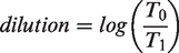
A reduction in the rate of poverty can be caused by a population dilution effect. This occurs where the number of people in poverty is unchanged (n₀ = n₁) but the total population grows (T₁ > T₀). In this case, the ratio between the two rates reduces to T₀/T₁. This ratio is positive and right-skewed, as for T₁ > T₀ it falls between 0 and 1, but for T₀ > T₁ it lies between 1 and infinity. Therefore, we ought to follow best practice for modelling positive-only variables and take logarithms before analysis. The dilution indicator therefore becomes

d i l u t i o n = l o g (\frac{T_{0}}{T_{1}})

A reduction in the rate of poverty can also be caused by a change in the number of people in poverty, and in the pure case, this occurs where there has been no change in the population denominator (T₀ = T₁). In this case, the ratio between the two rates becomes n₁/n₀. Again, we should take logarithms of this positive quantity arriving at

d i s p l a c e m e n t = l o g (\frac{n_{1}}{n_{0}})

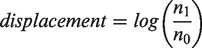
This displacement indicator can also be used as a measure of poverty concentration, i.e. an increase in distributional unevenness that occurs due to the absolute number of people in poverty increasing. Returning to our original ratio between the poverty rates and taking logarithms we can now see, using the algebraic rules of logarithms (i.e. log(AB) = logA + logB), that

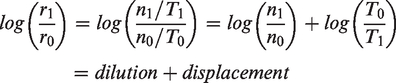
\begin{matrix} l o g (\frac{r_{1}}{r_{0}}) = l o g (\frac{n_{1} / T_{1}}{n_{0} / T_{0}}) = l o g (\frac{n_{1}}{n_{0}}) + l o g (\frac{T_{0}}{T_{1}}) \\ = d i l u t i o n + d i s p l a c e m e n t \end{matrix}

The dilution and displacement indicators therefore decompose changes in the rate of poverty between changes in the total population (dilution) and changes in the absolute number of people who are poor (displacement). The interest here lies in whether dilution or displacement of income poor households is occurring in the highest poverty areas within local authorities, driving an increase in distributional evenness. Therefore, the dilution and displacement indicators are calculated for the top fifth of highest poverty areas within each LA area, separately for each age group. Where dilution has occurred, we would expect log(T₀/T₁) to be negative and associated with a fall in the evenness index; where displacement has occurred, we would expect log(n₁/n₀) to also be negative and associated with a fall in evenness index. In the case where recession or austerity has caused an increase in the number of poor individuals, log(n₁/n₀) would be positive and associated with an increase in evenness indices. Therefore, in the model, we expect a positive coefficient between these indicators and the change in evenness. We can expect that there may be correlation between the independent variables in the model. For example, a shift to lower income households living in private rented housing may cause an effect that would also be measured by the displacement indicator, and a similar effect may occur for changing locations of social housing.

Figure 1 shows the distribution of the independent variables in the model, with standard deviations in parentheses. It shows that within most local authorities, there has been an increase in lower income households living in private rented housing and that there has been an increase in the distributional evenness of social housing. The dilution indicators for all age groups show that in the majority of LA areas, there has been a dilution effect. The displacement indicators are more mixed; for income poor individuals of working age, there is more evidence of a concentrating effect; for older people and children, more local authorities have seen a displacement effect. In the models, the dilution and displacement indicators were scaled to have zero mean and a standard deviation of 1; other variables were left on their original scale. In LA areas that already had a high degree of distributional evenness at the beginning of the observation period the change in evenness should be expected to be more limited. Therefore, the initial value of evenness at 2005 is also included in the modelling.

Figure 1.

Distribution of independent variables. Standard deviations are shown in parentheses.

A number of goodness of fit measures are used to evaluate the models. The statistical significance of individual coefficients is evaluated by means of t-values (i.e. the coefficient divided by its standard error). Values greater than 2 indicate statistical significance at the 95% level. Decreases in the Bayesian Information Criterion (BIC), a transformation of the log likelihood that penalises model complexity, are used to indicate improvements in the model, as are likelihood ratio tests of nested models. Explained variance is calculated according to a method proposed by Snijders and Bosker (2012). This is the reduction in total residual variance (i.e. the sum of variances at both levels) in the proposed model compared to the empty model with group structure only. The importance of group structure is evaluated in the empty model using the intra-class correlation coefficient (the ratio of between-group variance to total variance).

Findings

Children

Figure 2 shows how the three evenness indices have changed for child poverty between 2006 and 2014, based upon the CLIF indicator, by LA supergroup. Although they are at different levels with G > D > A9, the three indices are very closely related. The linear correlations between the measures are greater than 0.99 and the correlations between the three measures of change over the period are greater than 0.92. All LA area types show evidence of an increasingly even distribution of child poverty, though there are differences between areas types in the initial level of unevenness and the degree of change over time.

Figure 2.

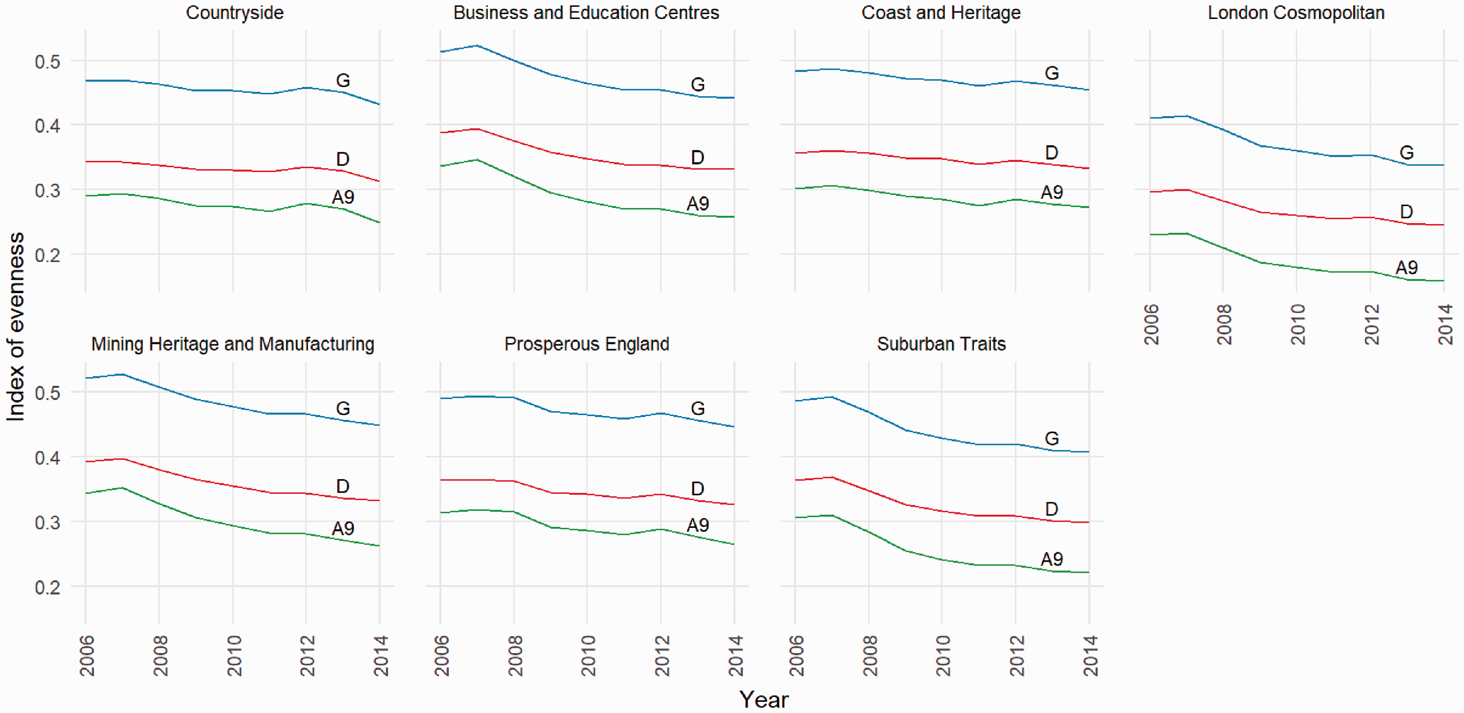
Evenness measures for CLIF child poverty indicator within LSOAs by English local authority supergroup 2005–2014.

The seven LA supergroups can be categorised according to their starting level of distributional evenness, focusing here on the Index of Dissimilarity D. The London cosmopolitan group of local authorities had the lowest initial level of D at 0.30. Local authority areas in the types ‘Coast and Heritage’, ‘Countryside’, ‘Prosperous England’ and ‘Suburban Traits’ had initial values of D between 0.34 and 0.36. The most uneven distribution of child poverty was found in ‘Business and Education Centres’ and ‘Mining Heritage and Manufacturing’ which both had initial D values of 0.39.

The evenness indices decreased most in the more urban LA types. In ‘London Cosmopolitan’ LA areas, D fell to 0.24 which was still the lowest of all LA supergroup types. In the ‘Business and Education Centres’, ‘Mining Heritage and Manufacturing’ and ‘Suburban Traits’ supergroup types, D fell between 0.06 and 0.07. The lowest declines in D were in the most rural supergroup types – ‘Prosperous England’, ‘Countryside’ and ‘Coast and Heritage’. Due to these different rates of change, by 2014 evenness measured by D in ‘Business and Education Centres’ and ‘Mining Heritage and Manufacturing’ LA types was 0.33, very similar to that in ‘Prosperous England’ and ‘Coast and Heritage’ local authorities. Very similar conclusions are drawn from an inspection of the other two indices, G and A9, and from the similar but temporally coarser IDID indicator. It is interesting to note that the evenness indices continued to decline in 2013 and 2014. These data points are unavailable for working age and pensionable age people.

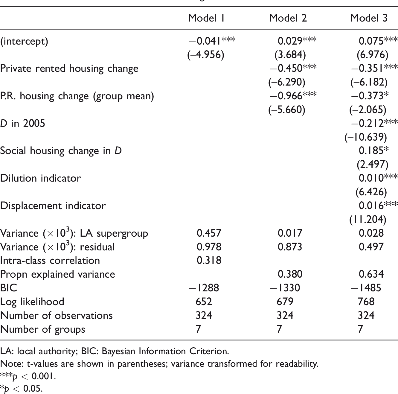
Table 1 shows the results from a hierarchical linear model of the change in evenness as measured by D between 2005 and 2012 using the IDID indicator. Given the differences in trend by LA type, we would expect the group structure to be important. This is indeed the case: the intra-class correlation in model 1 (the empty model with no independent variables) is 0.32, showing that around a third of the variance exists between LA types and two-thirds within them.

Table 1.

Hierarchical linear model of change in D 2005–2012 for children.

	Model 1	Model 2	Model 3
(intercept)	−0.041***(–4.956)	0.029***(3.684)	0.075***(6.976)
Private rented housing change		−0.450***(–6.290)	−0.351***(–6.182)
P.R. housing change (group mean)		−0.966***(–5.660)	−0.373* (–2.065)
D in 2005			−0.212***(–10.639)
Social housing change in D			0.185* (2.497)
Dilution indicator			0.010***(6.426)
Displacement indicator			0.016***(11.204)
Variance (×10³): LA supergroup	0.457	0.017	0.028
Variance (×10³): residual	0.978	0.873	0.497
Intra-class correlation	0.318
Propn explained variance		0.380	0.634
BIC	−1288	−1330	−1485
Log likelihood	652	679	768
Number of observations	324	324	324
Number of groups	7	7	7

LA: local authority; BIC: Bayesian Information Criterion.

Note: t-values are shown in parentheses; variance transformed for readability.

***p < 0.001.

*p < 0.05.

Model 2 includes the change in private rented tenure amongst lower NS-SeC households – as independent variables at both LA supergroup and individual LA levels. The coefficients on these variables are highly statistically significant in the model (p < 0.001). The direction of the relationship is as theoretically expected from section “The spatial distribution of income poverty: Evidence, theory and drivers”: D decreased more in those areas which had larger increases in the proportion of lower NS-SeC households in private rented housing. This relatively simple model explains 38% of the dependent variable’s variance and explains almost all the variance between LA supergroup types. The BIC criterion decreases, showing an improvement in the model, and a likelihood ratio test comparing models 1 and 2 also shows that the model 2 predictors are highly significant (chisq = 53.5, df = 2, p < 0.001).

Model 3 retains the model 2 explanatory variables and adds the initial value of D at 2005, the change in evenness of social housing, the dilution indicator and the displacement indicator. The coefficients for these indicators are statistically significant and the direction of the relationships is as theoretically expected. The proportion of explained variance increases to 63.4%, the BIC decreases compared to model 2 and a likelihood ratio test comparing the nested models 2 and 3 shows that these additional variables are statistically significant (chisq = 178.4, df = 4, p < 0.001). The coefficient on the private rented variable is attenuated in model 3 compared to model 2, which may be due to the correlation between explanatory variables. Social housing evenness and the dilution indicator were statistically significant at the group level, but explained only 2% additional variance so were omitted to keep the final model relatively parsimonious. The coefficient on the displacement indicator is larger than the dilution indicator coefficient, suggesting that an absolute decline in the number of poor children in the highest poverty areas has had a larger influence than dilution through population growth.

Working age people

For the sake of brevity, the charts and table for working age people are not included here as they illustrate similar patterns to those for children; the full set of material is provided as supplementary information. The values of D in 2005 by LA type are similar to those for children in both magnitude and rank order. It fell in most LA types, but fell by less than for children and there was no change in ‘Countryside’ and ‘Coast and Heritage’ LA supergroups. A hierarchical linear model with the change in private rented housing as independent variable explains 24.7% of the dependent variable’s variance, and the full model explains 63.4% (coincidentally, the same as the full model for children). The coefficients are all statistically significant and in the theoretically expected direction, with the displacement indicator appearing more important than the dilution indicator.

Older people

Figure 3 shows the evenness indices in 2005, 2008 and 2012 for the older age IDID indicator. The indices are in the same order as for other age groups (G > D > A9) and are closely correlated with each other. The smallest correlation between the three measures is 0.98 and the smallest correlation of change over the period (between D and A9) is 0.83. Change over time is more limited than the two younger age groups but with evidence of an increase in the indices. Again, change in D is focused on in the discussion below.

Figure 3.

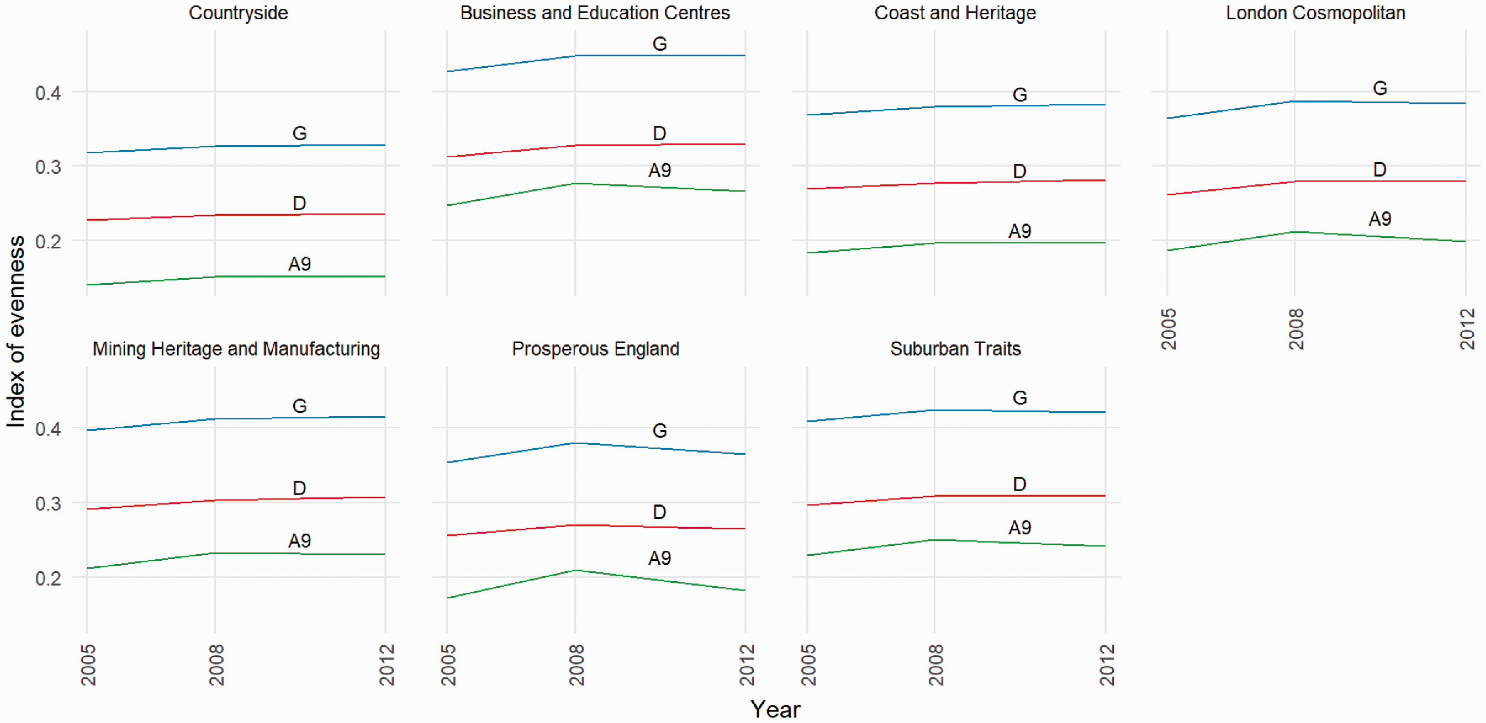
Evenness measures for older age IDID indicator within LSOAs by local authority supergroup 2005–2012.

The highest values of D are again found in ‘Business and Education Centres’ and ‘Mining Heritage and Manufacturing’ LA types, though these are lower than the younger age groups at 0.31 and 0.30, respectively. ‘London cosmopolitan’ LA areas do not stand out as having a particularly low value of D; ‘Countryside’ LAs have the lowest value in 2005 at 0.23.

All area types have an increase in D, but the change over the period is smaller than other age groups and less differentiated between LA types. The increase ranges from 0.008 (‘Countryside’) to 0.017 (‘London cosmopolitan’), with the most urban areas having the largest change. For most area types, the greater part of this change occurs between 2005 and 2008. No changes in rank order occur as a result of the increases between 2005 and 2012. Again, similar findings are reached by inspecting the other two indices.

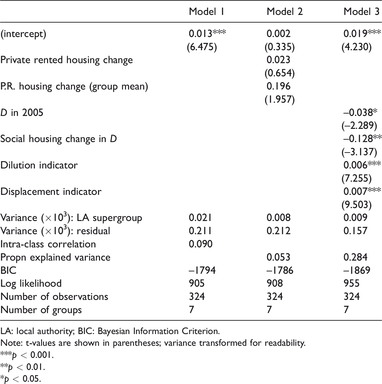
Table 2 shows the results from hierarchical linear models of the change in D between 2005 and 2012 for the older age IDID indicator. Given the smaller differentiation between LA types amongst this age group, we would expect the group structure in the model to be less important. The intra-class correlation in the empty model 1 shows that this is the case: just 9% of the variation in the dependent variable is between LA types.

Table 2.

Hierarchical linear model of change in D 2005–2012 for older people.

	Model 1	Model 2	Model 3
(intercept)	0.013***(6.475)	0.002 (0.335)	0.019*** (4.230)
Private rented housing change		0.023 (0.654)
P.R. housing change (group mean)		0.196 (1.957)
D in 2005			–0.038* (–2.289)
Social housing change in D			–0.128** (–3.137)
Dilution indicator			0.006*** (7.255)
Displacement indicator			0.007*** (9.503)
Variance (×10³): LA supergroup	0.021	0.008	0.009
Variance (×10³): residual	0.211	0.212	0.157
Intra-class correlation	0.090
Propn explained variance		0.053	0.284
BIC	–1794	–1786	–1869
Log likelihood	905	908	955
Number of observations	324	324	324
Number of groups	7	7	7

LA: local authority; BIC: Bayesian Information Criterion.

Note: t-values are shown in parentheses; variance transformed for readability.

***p < 0.001.

**p < 0.01.

*p < 0.05.

Model 2 includes the change in lower NS-SeC households in private rented housing. Theoretically, we do not expect a relationship with change in private rented housing at this age group, but it is explored here to confirm this expectation. Neither coefficient is statistically significant at the 5% level. The BIC increases, indicating a poor model fit, and the model explains just 5.3% of the variance. A likelihood ratio test indicates that this model is not an improvement on the empty model 1 (chisq = 4.1, df = 2, p = 0.127).

Model 3 excludes the private renting variable, adding the other four explanatory variables. All additional variables are statistically significant (with at least p < 0.01). The relationships with the dilution and displacement indicators are in the theoretically expected direction, but the relationship with change in social housing evenness is in the opposite direction. No variables were found to be statistically significant at the LA supergroup level. The BIC decreases and the model now explains 28.4% of the variance. A likelihood ratio test indicates that model 3 is an improvement over the empty model 1 (chisq = 99, df = 4, p < 0.001). The relative size of the coefficients suggests that increasing unevenness has been influenced by a growth in the absolute number of poor older individuals in the highest poverty areas and a loss of total population in those areas.

Discussion and conclusions

These results confirm the increasingly even distribution of income poverty observed in other studies of British cities. It also shows that these patterns, while stronger in the most urban English LA areas, are not confined to them, and that there is clear differentiation by age group. For children, the evenness indices declined in all LA supergroup types, the greatest falls being in the more urban LA types. For working age people, the falls in evenness indices were smaller than for children. There was no decline in the indices in the most rural LA types and again the greatest falls occurred in the most urban. For both these age groups, the increase in evenness was associated with an increasing proportion of lower income households living in private rented housing. This variable alone accounted for a large proportion of the variation in evenness change. Increasing evenness was also associated with higher initial levels of unevenness, an increasingly even distribution of social housing, and dilution and displacement processes in the highest poverty areas. The relative size of model coefficients suggests that an absolute fall in the number of income poor individuals in high-poverty areas had a greater influence than a dilution effect through total population growth, though both processes appear to be important.

For older people, the findings are rather different. Initial values of evenness indices were much lower than for the younger age groups. All LA types had an increase in the evenness indices between 2005 and 2012, though the change was small compared to the younger age groups. There was no relationship between private rented housing and evenness indices for pensionable age poverty evenness, as expected from the theoretical discussion and literature review. Increasing evenness was associated with dilution and displacement processes in the highest poverty areas, but these effects were much smaller than for the younger age groups.

The study also found that the three evenness indices used – the Index of Dissimilarity, the Gini coefficient and the Atkinson index – were very closely correlated and gave broadly similar results, despite their different properties. This suggests that the changes in evenness reported are happening across the whole distribution, rather than just in the highest or lowest poverty areas. The study covers a relatively short period of time, with three data points for working age and pensionable age populations; however, the annual time series derived from the CLIF child poverty indicator suggests that there has been a smooth increase in evenness over time that has continued up until 2014, the latest data point available. Although the explanatory variables derived from the Census do not exactly match the time span of the study, there are significant associations with the change in evenness.

The results of the modelling, plus the different patterns of distributional evenness by age group, suggest that increasing propensity for working age low-income households to be living in private rented housing is heavily implicated in the increasingly even distribution of income poverty in England over the period 2005–2014. This may be a consequence of choices by low-income households to rent their home in lower poverty neighbourhoods, or a mechanical result of the lower segregation of private rented compared to social rented housing. Alternatively, it may be the result of gentrification by displacement (Slater, 2009): low-income households being priced out of rented housing in urban neighbourhoods newly popular with a growing population of young, childless, higher income professionals. There is also evidence that lower income households are becoming more residentially dispersed as social housing is becoming less segregated from other types of housing, through mixed tenure developments or the siting of new build private housing near existing social housing.

It has been proposed by many researchers that outcomes for low-income individuals living in high-poverty areas are worse as a consequence of the neighbourhood they live in, i.e. that there are ‘area effects’. Do the findings of this research mean that area effects are reducing as mixed income neighbourhoods become an increasing reality? If area effects operate through peer networks there is a possible impact, though residence is but one place where people spend their time. The existence of within-neighbourhood or even within-building segregation would limit this, such as ‘poor doors’ in mixed-tenure buildings which provide separate entrances for private rented and social rented housing (Crossley, 2017: 38). If area effects operate via the quality of services and amenities, there may be positive benefits via an increase in ‘middle-class voice’ and reduced territorial stigmatisation. On the other hand, Cheshire (2009) argues forcefully that high-poverty areas can be viewed as ‘specialised neighbourhoods’ that create welfare by providing low-cost housing, services and support networks, and that mixed communities destroy this welfare. It may well be the case that mixed communities destroy certain types of social welfare but create others. More research could be conducted to understand these welfare gains and losses, both through quantitative ‘natural experiments’ and qualitative case studies.

‘Area-based initiatives’ targeted on high-poverty areas have been used to ameliorate area effects and also to target low-income individuals. At the start of the period covered by this study, approximately £1.5 billion was being spent annually on policies targeted at the ‘most deprived’ neighbourhoods (Lupton et al., 2013a: 15), but this was cut by the 2010 coalition government and replaced with a ‘new localism’ (Collins, 2016) in which local authorities were left to determine (and fund) neighbourhood policy. Area-based initiatives continue to be employed by local actors, but if income poverty becomes more dispersed these initiatives will be less effective means of reaching low-income individuals. The shift of low-income households into private rented housing means that in addition to increased dispersal, the location of low-cost housing and therefore low-income households can shift more quickly. Area targeting is typically undertaken using the Indices of Deprivation, now six years old; in the absence of up-to-date official statistics, local bodies must utilise their own sources of evidence to ascertain contemporaneous spatial patterns of poverty.

The impact on area effects and the efficiency of area-based initiatives depend upon whether the trend towards an increasingly even distribution of income poverty is permanent or simply a transitional phase. Bailey and Minton (2018) show that poverty has become a more suburban phenomenon in Britain and ask whether the increasingly even distribution of poverty is a temporary phase, as low-income households become displaced from newly popular inner city locations, and low-cost housing becomes situated in the suburbs.

This study does not provide incontrovertible evidence that lower income households are being displaced by higher income households. The displacement indicator used in the modelling shows that increasing distributional evenness is associated with an absolute decline in the number of low-income individuals living in high-poverty areas. This certainly could be caused by displacement of low-income households, but it could also be caused by in-situ changes in the risk of low income. Bailey (2012) reports that whilst selective migration is often assumed to be the dominant force in neighbourhood change, in-situ changes can also be important. Households at the lower end of the income distribution are becoming more like those in the middle in terms of tenure, employment and benefit income (Belfield et al., 2016: 53); it could therefore be the risk of poverty that is becoming more spatially dispersed, rather than the movement of individuals themselves.

Footnotes

Acknowledgements

The author is very grateful to three anonymous reviewers plus Ken Cleaver, Danny Dorling, David Kirk, Rachel Loopstra, Ludi Simpson and Dariusz Wojcik for offering comments on earlier drafts of this article. Data were derived from the English Indices of Deprivation 2007, 2010 and 2015 which are ©Crown copyright from the UK Department of Communities and Local Government. The latter dataset is published using the Open Government License (OGL) version 3.0. Use was also made of the 2011 ONS Local Authority Classification. Data from the 2001 and 2011 England and Wales Censuses were accessed via the Nomis website. Analysis was conducted in R version 3.3.2 with ggplot2, lme4 and texreg packages. The code is available at [].

Declaration of conflicting interests

The author(s) declared no potential conflicts of interest with respect to the research, authorship, and/or publication of this article.

Funding

The author(s) disclosed receipt of the following financial support for the research, authorship, and/or publication of this article: This work was supported by the Economic & Social Research Council (grant number ES/J500112/1); and the Engineering & Physical Sciences Research Council (grant numbers EP/K503113/1, EP/L505031/1, EP/M50659X/1).

References

Atkinson

(1970) On the measurement of inequality. Journal of Economic Theory 2: 244–263.

Bailey

(2012) How spatial segregation changes over time: Sorting out the sorting processes. Environment and Planning A 44(3): 705–722.

Bailey

Minton

(2017) The suburbanisation of poverty in British cities, 2004–16: Extent, processes and nature. Urban Geography 39(6): 892–915.

Batey

Brown

Pemberton

(2008) Methods for the spatial targeting of urban policy in the UK: A comparative analysis. Applied Spatial Analysis and Policy 1(2): 117–132.

Beatty

Fothergill

(2013) Hitting the Poorest Places Hardest – The Local and Regional Impact of Welfare Reform. Sheffield: Sheffield Hallam University.

Belfield

Cribb

Hood

et al . (2016) Living Standards, Poverty and Inequality in the UK: 2016. London: Institute for Fiscal Studies.

Bradshaw

Richardson

(2007) Spatial Variations in the Take-up of Means-Tested Benefits. London: Department for Communities & Local Government.

Catney

(2015) Exploring a decade of small area ethnic (de-)segregation in England and Wales. Urban Studies 53(8): 1691–709.

Cheshire

(2009) Policies for mixed communities: Faith-based displacement activity? International Regional Science Review 32(3): 343–375.

10.

Collins

(2016) Urban civic pride and the new localism. Transactions of the Institute of British Geographers 41(2): 175–186.

11.

Crossley

(2017) In Their Place: The Imagined Geographies of Poverty. London: Pluto Press.

12.

Dawkins

(2007) Space and the measurement of income segregation. Journal of Regional Science 47(2): 255–272.

13.

Department for Work and Pensions (2017) Households below Average Income: An Analysis of the UK Income Distribution: 1994/95–2015/16. London: Department for Work & Pensions.

14.

Dorling

Mitchell

Shaw

et al . (2000) The ghost of Christmas past: Health effects of poverty in London in 1896 and 1991. British Medical Journal 321(7276): 1547–1551.

15.

DWP (2016) Households below Average Income (HBAI) Statistics. London: Department for Work & Pensions.

16.

Fenton

(2016) Gentrification in London: A Progress Report, 2001–2013. CASE Papers. London: London School of Economics.

17.

Hanna

Bosetti

(2015) Inside out: The New Geography of Wealth and Poverty in London. London: Centre for London.

18.

HMRC (2012) Child Benefit, Child Tax Credit and Working Tax Credit: Take-up Rates 2011/12. London: HM Revenue & Customs.

19.

HMRC (2014) Children in Low-Income Families Local Measure. London: HM Revenue & Customs.

20.

Hochstenbach

(2017) State-led gentrification and the changing geography of market-oriented housing policies. Housing, Theory and Society 34(4): 399–419.

21.

Hochstenbach

Musterd

(2018) Gentrification and the suburbanization of poverty: Changing urban geographies through boom and bust periods. Urban Geography 39(1): 26–53.

22.

Iceland

Weinberg

Steinmetz

(2002) Racial and Ethnic Residential Segregation in the United States: 1980–2000. Washington, DC: U.S. Government Printing Office.

23.

James

Taeuber

(1985) Measures of segregation. Sociological Methodology 15: 1–32.

24.

Kavanagh

Lee

Price

(2016) Is poverty decentralising? Quantifying uncertainty in the decentralisation of urban poverty. Annals of the Association of American Geographers 106(6): 1286–1298.

25.

Leeser

(2016) English Indices of Deprivation 2015. London: Greater London Authority.

26.

Lupton

Fitzgerald

(2015) The Coalition’s Record on Area Regeneration and Neighbourhood Renewal 2010–2015. Social Policy in a Cold Climate. London: London School of Economics.

27.

Lupton

Fenton

Fitzgerald

(2013a) Labour’s Record on Neighbourhood Renewal in England: Policy, Spending and Outcomes 1997–2010. Social Policy in a Cold Climate. London: London School of Economics.

28.

Lupton

Vizard

Fitzgerald

et al . (2013b) Prosperity, Poverty and Inequality in London 2000/01–2010/11. London: London School of Economics.

29.

Manley

Ham

Bailey

et al . (2013) Neighbourhood effects or neighbourhood based problems? In: Manley D, van Ham M, Bailey N, Simpson L, Maclennan D (eds) Neighbourhood Effects or Neighbourhood Based Problems? a Policy Context. London: Springer, pp.1–23.

30.

Massey

Denton

(1988) The dimensions of residential segregation. Social Forces 67(2): 281–315.

31.

Meen

Gibb

Goody

et al . (2005) Economic Segregation in England. York: Joseph Rowntree Foundation.

32.

Nolan

Whelan

(1996) Resources, Deprivation and Poverty. Oxford: Oxford University Press.

33.

Rae

(2013) English urban policy and the return to the city: A decade of growth, 2001–2011. Cities 32: 94–101.

34.

Reardon

O’Sullivan

(2004) Measures of spatial segregation. Sociological Methodology 34: 121–162.

35.

Slater

(2009) Missing Marcuse: On gentrification and displacement. City 13(2–3): 292–311.

36.

Smith

Noble

et al . (2015a) The English Indices of Deprivation 2015 – Technical Report. London: Department for Communities & Local Government.

37.

Smith

Noble

et al . (2015b) The English Indices of Deprivation 2015: Research Report. London: Department for Communities & Local Government.

38.

Snijders

TAB

Bosker

(2012) Multilevel Analysis: An Introduction to Basic and Advanced Multilevel Modelling. London: Sage.

39.

Tinson

Ayrton

Barker

et al . (2016) Monitoring Poverty and Social Exclusion 2016. York: Joseph Rowntree Foundation.

40.

Tunstall

(2016) Are neighbourhoods dynamic or are they slothful? The limited prevalence and extent of change in neighbourhood socio-economic status, and its implications for regeneration policy. Urban Geography 37(5): 769–784.