Bridging the gap between geographic concept and the data we have: The case of labor markets in the USA

Abstract

A broad literature has made it clear that geographic units must be selected with care or they are likely to introduce error and uncertainty into results. Nevertheless, researchers often use data “off the shelf” with the implicit assumptions that their observations are consistent with the geographical concept relevant for their research question, and that they are of uniformly high quality in capturing this geographic identity. In this paper, we consider the geographical concept of “labor market” and offer a template for both clarifying its meaning for research and testing the suitability of extant labor-market delineations. We establish a set of metrics for comparing the quality of existing labor-market delineations with respect to the diverse meanings that researchers apply to the concept. Using the fit metrics established here, researchers can explore how delineations vary geographically, how they vary over time, and how this variation may shape research outcomes. Our assessment is that the quality of the extant delineations is relatively high overall. However, we find that different delineations vary significantly in the types of labor markets they represent, and that regional variations in fit within any given delineation may introduce noise or regional bias that merits consideration in any analysis conducted with these units. More broadly, the kinds of metrics we propose here have applicability for many other geographic entities where boundaries and scale can be only imperfectly defined.

Keywords

Geographic uncertainty labor markets regional analysis

Motivation

A fundamental tenet of geographic research is that outcomes are shaped by geographic context. A key challenge for geographers has been to define meaningful observations so that these contextual effects can be observed and understood. A “spatial turn” in the social and health sciences has vastly increased the visibility of spatially explicit analyses that assign meaning to geographical context (Warf, 2017). This increased visibility requires continued input on the nature and quality of the observations being employed (Kwan, 2012).

The study of neighborhoods and neighborhood effects provides a clear blueprint for what a careful engagement with the nature and quality of geographical observations should look like. Numerous studies have examined the impact of certain kinds of neighborhoods on a range of social, economic, and health outcomes (Chaix et al., 2013; Crowder and Krysan, 2016; Hwang, 2015; Johnson et al., 2002; Leventhal and Brooks-Gunn, 2003; Ludwig et al., 2013; Sampson, 1997, 2019). In parallel with this focus on neighborhoods, researchers have raised concerns—both old and new—about how neighborhoods are defined and what kinds of uncertainty might enter an analysis because of the imperfect translation of theoretical concept to data product (Galster, 2019; Kwan, 2012; Openshaw and Taylor, 1981; Zenk et al., 2011). Researchers have also provided methods for examining this uncertainty (Fowler et al., 2019; Spielman and Folch, 2015) and estimating its effects on outcomes (Fotheringham and Wong, 1991; Root et al., 2011), as well as new data products and methods that may help to alleviate some of the problems (Johnston et al., 2016; Logan et al., 2014; Östh et al., 2014; Schroeder, 2007).

Labor-markets are conceptually similar to neighborhoods in that they make theoretical sense as a unit of observation but are devilishly hard to define. Nevertheless, labor markets have garnered little attention over the years as to the validity of their conceptual frame or the robustness of extant delineations. Labor markets exist because of the particularities of economic agglomeration, work practices, residential settlement patterns, and a host of other complexities all coming together in a region. Which of these particularities is most important will vary across research questions, but at a minimum we must recognize that the drawing of labor-market boundaries will require significant assumptions and that our observations will vary in quality with respect to these assumptions. Compounding this uncertainty, we have only limited data on workers, firms, behaviors, and histories from which to construct our observations, meaning that any incapacity to measure and define will further degrade the link between concept and observation. The solution, as with neighborhoods, is not to abandon the geographical concept but rather to approach our observations cautiously, with a clear conceptual framing, a detailed knowledge of data quality, and a willingness to explore the impacts of uncertainty on our findings. While applied specifically to the concept of labor market here, our intent is to offer a generalizable process that could be applied to any number of constructed geographic units from neighborhoods and metros to (non-state defined) territories, regions, and hinterlands.

In this paper, we explore the different meanings researchers have attached to the concept of labor market, develop a series of metrics that will allow us to test the relationship between concept and fit for a particular labor-market delineation, and provide resources for researchers to examine the quality of extant delineations. By providing a theoretical frame for understanding labor markets and a set of statistics for examining the quality of our observations, we hope not only to advance the use of labor markets as a unit of observation but also to provide a framework for the responsible use of aggregate geographic data more generally. Despite decades of work on issues such as the modifiable areal unit problem, the practice of taking spatial units as given and unproblematic is still widespread. If we are to appreciate fully the significance of contextual variables on a range of outcomes, we will need to be better at knowing what contexts we are measuring and how well we measure them.

Labor markets

Our ability to delineate and understand the bounds of labor markets confidently has value for governments and researchers alike. Having an accurate labor-market delineation can inform decisions related to qualification for government programs, regional development, economic planning, and regional marketing (Fowler and Kleit, 2014; Jones and Paasi, 2013 citing Smart, 1974; Pike, 2011; Van Nuffel, 2007). Researchers rely on labor-market delineations to understand variation in earnings across industries and gender (Gibbs and Bernat, 1998; Tickamyer and Bokemeier, 1987), the relationship between education and unemployment (Killian and Parker, 1991), and factors associated with firm formation (Armington and Acs, 2010), among many others.

Despite the important role labor-market delineations have played in both research and policy analysis applications, there has been little attempt to assess their validity internally, over time, or comparatively (but see Foote et al., 2017; Plane, 1981; Tong and Plane, 2014). Different delineations tend to be favored within particular research areas (e.g., commuting zones within rural sociology) and their utilization creates an incentive to use them again if only to create comparable results. For the most part, however, both researchers and government agencies use these delineations with little consideration of how well the delineations match the conceptual model of a labor market that they intend.

The most widely used US labor-market delineations all share some important features, but it is critical to recognize that they were each created for slightly different reasons. More broadly, the concept of “labor market” is not monolithic. Indeed, a half-century ago, J.F.B. Goodman (1970: 179) noted that “the labour market is a term which is often used loosely, and which suggests a unity absent in practice.” If we want to understand how well or poorly existing delineations match the concept of labor market, we must first “look under the hood” and define our terms. While some applications will focus on the agglomerative properties of major economic engines and be “core” focused, others may emphasize the degree to which counties are “connected” or the degree to which individuals are likely to both live and work in the same labor market (e.g., “contained”). Our paper thus begins by exploring these competing definitions of labor market and identifying the kinds of measures one might employ to assess whether a given delineation fits a particular definition.

Defining theoretical models of labor markets and the measures to assess fit is an important first step. The logical next step is, of course, to test these delineations for fitness. Indeed, Casado-Diaz and Coombes (2011: 24) who have undertaken important work on how to best delineate labor markets write that “there still needs to be a systemic study of the ‘performance’ of different methods” of labor-market delineation. Despite a long history of application for research and policy analysis, there are significant and known uncertainties about these delineations that trace to a number of sources, including the intentions behind the original delineation, geographic variation in how well the labor-market concept applies, and changes in the data used to define and measure labor markets.

The first example of a known source of uncertainty lies in variation among delineations based on what purpose they were meant to fulfill. The most obvious of these in the U.S. context is between the Office of Management and Budget (OMB)’s (2010) core-based statistical areas (CBSAs), which focus on core population agglomerations, and the USDA Economic Research Service (ERS)’s commuting zones (CZs), which were meant to focus on the connectivity of rural places. As a result of these differing starting points, the CBSA delineation excludes many smaller and more remote counties, while the CZ delineation emphasizes whatever connections these counties might have to fit them into a labor market.

Second, there is uncertainty about the variation in quality within delineations. Because counties and core areas vary in size and distance from one another and because people’s economic behavior with respect to employment and commuting also changes over time, we should expect commensurate variation in the quality of observations geographically, over time, and by metropolitan size. Nearly 40 years ago, Plane’s (1981) work made it clear that the labor-market concept applied poorly to New England where the density of core areas resulted in overlapping commuting patterns that would be unusual in other parts of the country. Within any delineation, there will be geographic regions that match the theoretical model of labor market better, but to our knowledge, there are no published characterizations of variation in quality within delineations or across the same delineation over different years.

Finally, the data on county-to-county commuting flows that is used to delineate labor markets in the USA fundamentally changed between 2000 and 2010 when the Census Bureau switched from the 5% sample of the decennial long form to the 2% sample of the American Community Survey (ACS). Similarly, the OMB significantly revised the standards for identifying “core” counties between 2000 and 2010. The changed core designation significantly changes how we view the economic landscape and ultimately how we judge the quality of delineations. Despite the fact that all of this uncertainty and variation is known to be an issue, we are not aware of any effort to compare and contrast the effect of changed data quality systematically on internal and cross-delineation measures of fit.

This paper makes three contributions to the use of labor markets as a unit of observation. We first distinguish among labor-market definitions to gain some conceptual clarity on what we wish to measure. Next, we designate a set of easily explained measures of fit that we feel can be used to distinguish quality between and within delineations. Finally, we compare a set of extant US labor-market delineations based on these metrics. Additionally, we make all of the delineations with associated fit statistics available online in a single location and provide an interactive map that allows users to compare and contrast these delineations in a variety of ways.¹ While the application here is to labor markets in the USA, there are obvious parallels to a broader set of “functional region” delineations employed in other parts of the world, and our insistence on clarity in the conceptual model and measurement of fit can be applied equally well to those contexts and to a broad set of constructed geographic regions (Casado-Díaz et al., 2016; Halás et al., 2016, 2018; Kropp and Schwengler, 2016).

Conceptual clarity: metropolitan areas, labor market areas, and labor-sheds

Appropriate use of geographical units of observation begins from a clear understanding of what those units signify. There are three main definitions of labor market implied (though rarely stated explicitly) in regional analysis: the metropolitan area, the labor market area, and the labor-shed. For the purposes of distinguishing among them, we propose a classification system, shown in Table 1, which differentiates the importance of a core economic area (i.e., core), the degree to which economic connectivity (e.g., wage similarities or coordinated shifts in employment rates) is assumed to be present within the region (i.e., connection), and the degree to which residents of the labor market are also assumed to work there (i.e., containment). These classifications provide a useful heuristic for researchers to enunciate what is being valued within an otherwise muddy term. We do not propose these terms for wider adoption (as they already have wide use in many contexts) but rather suggest them as tools for clarifying the link between research questions and appropriate units of analysis.

Table 1.

Characteristics of different labor market definitions.

	Core	Connection	Containment
Metropolitan area	Most important	Important	Not important
Labor-market area	Important	Most important	Important
Labor-shed	Not important	Not important	Most important

The metropolitan area approach is the most clearly defined and widely used of our three terms. The OMB has provided the census with metropolitan statistical area (MSA; formerly known as standard metropolitan areas and standard metropolitan statistical areas) delineations since the 1950s (United States Census Bureau, 2016). The existence of a central “core”—characterized by dense population and presumably dense economic activity—is essential to the metropolitan area treatment of labor markets. The origins of this focus extend at least back to Marshall’s (1890) focus on agglomeration economies, and its importance can also be seen in early sociological models of population sorting such as that of Park and Burgess (1925). Regional analysis focusing on metropolitan areas tends to take the urban core as the central object of study with other subregions attached because they form the core’s hinterland (Gabe, 2006; Ganning et al., 2013). Connectivity for these peripheral regions will therefore also be important as well. However, other concerns related to labor markets such as the treatment of polycentric urban areas or the degree of overlap between adjacent metropolitan areas are relatively less important.

Because of its importance within economic analysis, we use the term “labor-market area” here to refer to observations where the high density of commuting relationships among subunits suggests that changes in the supply of or demand for labor in one subregion would be felt equally within other subunits within the region (e.g., Garloff et al., 2011; Vanheuvelen, 2018). Related to critical assumptions about how wages and the supply of labor interact in space (Mas-Colell et al., 1995), the partitioning of subareas into distinct regions that move together is fundamental to much of economic analysis and explains both the motivation for the Bureau of Economic Analysis (BEA)’s early decision to develop labor-market areas and their relative popularity in both economics and regional science (Foote et al., 2017). In practice, highly connected labor markets are usually associated with the presence of a core or cores that anchor this connection, but for our purposes here, a labor-market area is primarily validated by correlations in wages among subunits within the labor-market area.

Finally, we use labor-shed to mean a “line enclosing the area which supplies workers to a workplace” (Green, 2009: 83). In this conception, containment dominates. For many types of analysis, particularly those with a rural focus, the issue is to find the larger boundary of possibility in which labor decisions may happen. The emphasis is on the possibility of connection more so than the presence of significant connection. The labor-shed concept, with its focus on possibility rather than connection or cores, may be important if, for example, one wanted to determine where people could go if they needed to look for work. The ERS’s CZs, with their emphasis on connecting rural areas to employment centers even in the context of very light commuting flows, are a prime example of how this definition has been delineated into a usable form and ultimately incorporated into research (Chetty et al., 2014; Fowler and Kleit, 2014; Gibbs and Bernat, 1998).

Labor markets do not exist in some ideal form that can be accessed through the right delineation. Instead, researchers need to be clear about the goals of their analysis, the spatial extent the processes they are studying might be expected to have, and the trade-offs they are willing to make in terms of delineation “fit” with their research goals. Different kinds of geographic units such as “metropolitan areas” and “neighborhoods” share this indeterminacy. Depending on the research goal, peripheral areas may or may not be relevant. Polycentricity may complicate the determination of a center or the boundaries between observations. These are matters of theoretical framing and need to be explicitly considered in geographic research of many types. That some places will fit the theoretical frame of a research question well and others will not is a factor in how we conduct our analyses. To consider this kind of variation, we need to be clear about our theory, but we also need to devise metrics that will allow us to examine and compare our observations. In the next section, we identify metrics to support researchers in making these choices.

Assessing the quality of labor markets: descriptive and fit statistics for regions and subregions

The ability to delineate labor markets accurately is contingent on several constraints. The arrangement of work and residence varies across place and time, meaning that the scale and fit of delineations will also vary geographically and temporally. Physical characteristics of the landscape and historical patterns of settlement condition the extent to which labor markets are distinct or overlap, furthering the variation in fit geographically. Counties, the building blocks of the delineations considered here, are also heterogeneous in size and population. Taken together, these constraints ensure that any labor-market delineation is likely to vary in quality and that this variation is likely to have a spatial pattern to it. Responsible use of labor markets must therefore consider the variation in this quality and take reasonable steps to minimize its impact on analytic results. Remarkably, with very few exceptions, the delineations currently available for US labor markets are made available to users without any reported validation, leaving analysts to assume that the delineation they are using is valid and appropriate (but see Foote et al., 2017; Fowler et al., 2016; Tong and Plane, 2014).

Researchers need to balance priorities when delineating labor markets, and the metrics presented here are intended to permit researchers to find a balance suited to their specific analysis. To increase the share of the population living and working in the same labor market (i.e., containment) requires delineating larger labor markets. Conversely, reducing the number of counties only weakly tied to their labor market requires increasing the number of labor markets or leaving counties out of the analysis. Distinguishing between labor-sheds and labor-market areas requires separating the degree to which a delineation contains its resident workforce—which can occur without significant commuting between counties—from the degree to which subunits move together economically (i.e., connection), which emphasizes dense connections and potentially penalizes subunits where most residents live and work in the same county. For some analyses, culling out counties that are not connected to an economic core will be appropriate (i.e., core-based), while for others, the presence of a metropolitan center is not essential to understanding economic connectivity. Any delineation will require the analyst to find a balance that optimizes on the combination of these and other criteria. Table 2 summarizes our proposed set of criteria for evaluating the quality of a given labor-market delineation and their associated justification. For the sake of brevity, more detailed support and explanation of these criteria is available in the Supplemental Appendix, and an R script for reproducing all of the metrics is provided on the project Web site at https://sites.psu.edu/psucz.

Table 2.

Measures for judging the quality of labor market delineations.

	Property and measures	Justification
Descriptive measures	Completeness
	Number of counties covered by delineation	A delineation should cover as much of the study area or study group as possible
	Population covered by delineation
	Size and shape
	Range, variation, and skew in area	While land area, population size, and number of counties will necessarily vary because regions vary, extreme outliers may indicate problematic groupings that prevent a useful comparison of observations
	Range, variation, and skew in population
	Range and variation in number of counties per labor market
	Compactness (Iso-Perimeter Quotient)Contiguity	While regions will take on a wide range of forms based on variation in the underlying counties, it is desirable that these shapes be as compact as possible and spatially contiguous except where counties are islands
	Spatial variation of fit measures
	Spatial clustering (Moran’s I) of labor market and county fit statistics	If “better” observations are clustered geographically, then this may bias subsequent analyses

Core	Share of metropolitan areas split into multiple labor markets	The concept of a unified core of economic activity means that most metropolitan areas should not be split
	Share of observations not containing at least one metropolitan or “core” county	For delineations which take an economic core as an essential component for understanding labor markets, there should be at least one county designated as “core”
	Average share of county residents who work in a core county of the labor market	When a delineation is core focused, labor-market residents will be more likely to work in core counties
	Average sum of share of county residents who work in core county plus share of county workforce that lives in a core county)	Counties are included in a CBSA if the combined share of their residents working in core counties and share of their workforce residing in core counties in the labor market is at least 25%; this measure reproduces that criterion

Connection	Correlation in average annual wage rate among counties in the same labor market over a six-year period	A key assumption for dense labor markets is that strong commuting patterns will lead to convergence in wages, as workers can seek employment anywhere within the region; similar measures based on, for example, unemployment rates could also be included here

Containment	Share of labor market residents who work in labor market (home containment)	Labor markets may be understood as regions of possibility with respect to employment; workers who cross labor market boundaries are problematic for this definition
	Share of labor market jobs filled by labor market residents (work containment)
	Share of US population that lives and works in same labor market

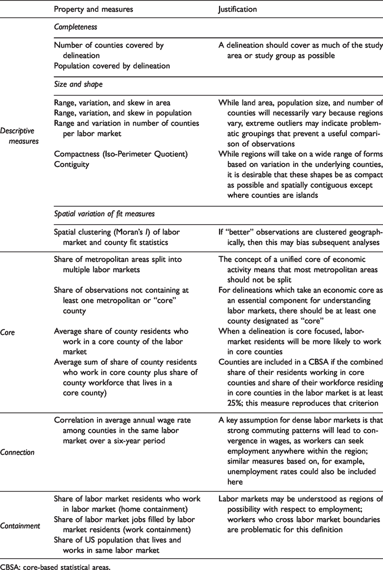
CBSA: core-based statistical areas.

Data

This paper compares delineations of labor markets from the OMB, ERS, and BEA, and also includes modifications of these delineations by Tong and Plane (2014) and Fowler et al. (2016). All of the delineations described here for each decade from 1980 through 2010 are assembled with complete metadata and documentation at https://sites.psu.edu/psucz. The OMB delineations include definitions for combined metropolitan statistical areas (CMSAs) and MSAs for 1980 and 1990, and CBSAs for 2000 and 2010 (United States Census Bureau, 2016). ERS CZ delineations for 1980, 1990, and 2000 were initially accessed through the ERS Web site (Economic Research Service, 2015). The 2010 delineation is based on a replication of the ERS methodology completed by Fowler et al. (2016). BEA economic areas were initially accessed via the Federal Communications Commission Web site (Federal Communications Commission, 2010) and conform to delineations by the Regional Economic Analysis Division of the BEA. Additional BEA delineations for 1977 and 1995 were obtained as a spreadsheet via personal communication with BEA staff. The delineations by Tong and Plane were made available by the authors. A full description of their method of linking counties in a way that accounts for polycentricity in urban form is the focus of their 2014 paper.

As our primary focus is establishing fit statistics for previously released delineations of labor markets, we follow previous research and use county-to-county commuter flow data made available through the ACS and the decennial census long form. We use data from the 1980, 1990, and 2000 census long form to provide base data for our analyses in these decades, and 2008–2012 data from the ACS for our 2010 analysis. Until 2000, commuting data had been collected using the census long-form questionnaire (question 22 in both 1990 and 2000 surveys) that asks “At what location did this person work last week?” (United States Census Bureau, 2000; emphasis in the original). Beginning in 2003, this question was moved to the ACS. Whereas this question was previously asked of 5% of the entire population every 10 years, it is now asked of only 2% of individuals and is administered continuously so that estimates are developed over multiple years. Because of collection methods, ACS data also capture seasonal employment trends and economic cycles. In addition, the question changed slightly to ask the respondent to provide the location of the place where they worked the most hours last week, including the address, county, and state. The census then geocodes this response to the “place” level and ultimately to the block and county level (McKenzie, 2013). Due to very partial data availability and limited inclusion in delineations, we exclude cases for Puerto Rico and other outlying US territories.

It is worth noting that the research conducted here, and by the authors in related projects, indicates that the structure of commuting data changed substantially between the 2000 census and the 2008–2012 ACS file. Some of this can be attributed to changing commuting practices associated with, for example, telecommuting, expansion of suburbs, suburb-to-suburb commuting flows, and reverse commuting flows. However, the impact of the changed survey method and sample size is likely significant. As Table 3 indicates, the number of CZs identified using the same ERS methodology was in decline from 1980 through 2000, but dropped significantly in the 2010 delineation. The degree to which the changes in these data reflect “real” changes in the structure of employment in the USA versus changes in survey methodology are not known. The implication for this research is that comparisons between delineations of the same year should be relatively straightforward, but comparisons between 2000 and 2010 delineations should be viewed with some caution.

Table 3.

Descriptive statistics.

				Population (000s)					Area (000s of km²)					Counties
Delineation	Year	N	Complete	Included	Min.	Mean	Max.	Kurtosis^e	Min.	Mean	Max.	Kurtosis^f	Compactness^g	Min.	Num. single	Mean	Max.
ERS^a	1980	765	Yes	100%	0.5	296	11,787	0.15	0.2	11	282	205.5	0.46	1	88	4.0	23
	1990	741	Yes	100%	1.3	336	14,545	−0.02	0.2	11	140	40.45	0.45	1	62	4.2	19
	2000	709	Yes	100%	1.2	397	16,393	0.08	0.2	11	140	38.36	0.45	1	47	4.4	19
ERS Mod.^b	2010	625	Yes	100%	1.0	494	17,877	0.05	0.3	13	133	24.72	0.49	1	40	5.0	20
ERS Rep.^b	2010	658	Yes	100%	1.0	469	17,877	0.1	0.3	12	172	43.23	0.50	1	33	4.8	20
BEA^c	1980	183	Yes	100%	110	1238	17,899	0.43	2.9	44	282	6.91	0.38	2	0	16.9	67
	1990	172	Yes	100%	60	1446	23,919	0.31	6.8	47	282	5.7	0.35	1	1	18.3	77
	2000	179	Yes	100%	83	1572	22,315	−0.09	7.0	45	286	7.34	0.35	1	1	17.5	83
	2010	179	Yes	100%	80	1725	23,154	−0.16	7.0	45	286	7.34	0.40	1	1	17.6	83
OMB CBSAs	2010	917	No	94%	13.5	316	19,567	1.24	0.3	5	71	30.38	0.45	1	602	2.0	29
Tong and Plane^d	2010	933	No	94%	12.1	310	18,897	1.32	0.3	5	71	29.47	0.59	1	621	2.0	33
−Metro only	2010	363	No	84%	55.3	712	18,897	0.89	0.4	7	71	20.44	0.52	1	146	3.3	33
−Micro only	2010	570	No	10%	12.1	54	243	−0.02	0.3	3	55	47.84	0.63	1	475	1.2	7

^aOriginal ERS delineations.

^bDelineations completed by Fowler et al. (2016).

^cBEA economic areas were delineated in 1977, 1995, and 2004. The 1977 delineation is used with the 1980 flows, the 1995 delineation is used with 1990 flows, and the 2004 delineation is used with both 2000 and 2010 flows.

^dDelineations based on Tong and Plane (2014).

^eKurtosis of population calculated on log of population, as we expect functional regions to be distributed on an exponential scale (Zipf, 1949).

^fKurtosis of area calculated on area in 1000s of square kilometers.

^gMean compactness based on IPQ method, as described in Li et al. (2013).

ERS: Economic Research Service; BEA: Bureau of Economic Analysis; OMB: Office of Management and Budget; Mod.: a modification meant to replicate the intent of the ERS analysis; Rep.: an exact replication of the ERS methodology.

Data on commuting flows for 1990, 2000, and 2010 (i.e., 2008–2012 ACS) were available from the Census Bureau Web site (United States Census Bureau, 2017), but 1980 data were not available from that source. For 1980, we utilized a file produced by the BEA in the mid-1980s. While the Census Bureau defined 3137 counties or county equivalents in 1980, the BEA data came with a number of counties combined.² In all cases, these combinations fell within the same metropolitan boundaries for the OMB definition, and the same economic areas for the BEA delineation. In all but two cases, these counties were also placed in the same labor-shed in the 1980 ERS delineation. So, very few discrepancies occurred in calculating descriptive or fit statistics. The two exceptions are Kalawao County, HI, which is joined here with Maui County, HI, and Martinsville City, VA, which is joined here with Henry County, VA. In both cases, the pairing of counties into a single unit used by the BEA in 1980 is mimicked in the ERS delineation for 1990 where those counties appear in the same CZs. When all exclusions and combinations were completed, the final data set has 3096, 3141, 3141, and 3143 county and county equivalencies for the decades 1980 through 2010, respectively.

Wage data for calculating pairwise correlations are published by the Bureau of Labor Statistics as part of their quarterly census of employment and wages and are available from as early as 1975 (Bureau of Labor Statistics, 2019). The analysis here relies on data from 1980–1985, 1990–1995, 2000–2005, and 2010–2015. As annual data, they require some manipulation to account for changes in county boundaries that occurred between census years and to match to the units used by the BEA for the 1980 analysis. The details of these changes are documented in the replication code included with this analysis.

Descriptive comparison of delineations

Table 3 conveys a range of descriptive statistics meant to highlight the differences in coverage, typical unit size, and compactness for the delineations considered here. The intent of these statistics is not to judge the quality of the delineation but rather to highlight the differences in intent that are visible from this type of comparison.

Completeness

The ERS and BEA delineations cover all 50 states.³ Only the OMB CBSA delineation includes outlying territories such as Puerto Rico or Guam. While it includes a broader set of counties in its set of potential labor markets, by intent, it defines labor markets for a much smaller set of counties overall. The OMB designation and its close relative suggested by Tong and Plane (2014) do a surprisingly good job of covering the vast majority of the country’s population (94%), even though they omit a substantial number of counties. OMB definitions for CMSAs include 761 counties in 1980 and 854 in 1990, while the more comprehensive CBSA boundaries for 2000 and 2010 include 1764 and 1808 counties, respectively. The Tong and Plane delineation, which covers only 2010, includes 1196 metropolitan counties and 701 micropolitan counties for a total of 1897 included counties. Given the population coverage of these delineations, many researchers may find the simplicity of the OMB CBSA delineation appealing for analyses based on data for 2010 or later. The limitation of the CBSA definition lies primarily in its limited time frame and its omission of many rural counties. The OMB has distributed a closely related delineation in previous decades (e.g., CMSAs and MSAs), but those delineations do not utilize the same criteria. A retroactive application of the CBSA definition could be undertaken, given the metropolitan core/non-core designations and the commuting connection provided with the supporting data, but such an effort goes beyond the scope of this paper.

Size (of population, land area, and number of counties)

Table 3 also describes the variation in size of the labor-sheds delineated in each methodology. The most significant point to draw from this comparison is that the delineations are remarkably similar along the range of these metrics, except for the BEA economic areas, which are much larger units. Put another way, a diverse range of techniques for dividing up the country into labor markets has led to substantially similar units in terms of population, area, and number of counties, suggesting some degree of robustness in the labor-market concept. While the CBSA delineations are missing some of the low-end labor markets in population terms (the smallest population CBSA was approximately 13,000 individuals compared to 1000 for the 2010 ERS delineation), they are otherwise remarkably similar. The average economic area, by comparison, has three to five times the population of the other delineations, and the largest economic area has more than twice as many counties as the largest CBSA and more than three times as many counties as the largest ERS CZ. This decision to group more counties together will make sense for some research applications where the priority is on not separating connected regions, but it will likely prove too large for other applications where grouping unlike counties into the same labor market is a more pressing concern. Additionally, the huge size of some of the BEA units may lead to concerns about the number of observations available for analysis and about coherence of the amalgamated observations.

Fit statistics

Table 4 compares delineations based on the measures of fit proposed in Table 2. The table describes fit in three different domains: core measures, connection measures, and containment measures. The measures describe the characteristics of the labor markets in each delineation (although related measures are also calculated for individual counties and made available with the rest of the supporting materials). Which fit statistics will be most relevant will depend on the analysis for which the delineation is being used. However, some general information about the suitability of each delineation can be ascertained from the table.

Table 4.

Fit statistics.

Delineation	Year	Core measures						Connection measures				Containment measures
		Metros split^e	Labor markets with core county	Share working in a core county^f		Commuting to or from a core county^f		Average pairwise wage correlation				Containmentⁱ				Population containment
				Share working in a core county^f		Commuting to or from a core county^f		Average pairwise wage correlation				Home			Work
				Mean	I ^g	Mean	I ^g	Min.	Mean	Mean 2+ ^h	I ^g	Min.	Mean	I ^g	Mean
ERS^a	1980	26	32%	13%	0.25	25%	0.28	0.10	0.93	0.92	0.05	62%	93%	0.35	95%	95%
	1990	33	35%	15%	0.28	28%	0.32	0.14	0.90	0.89	0.14	67%	90%	0.37	92%	94%
	2000	39	38%	17%	0.26	30%	0.31	0.19	0.91	0.91	0.06	62%	88%	0.29	91%	93%
ERS Mod.^b	2010	36	78%	40%	0.37	76%	0.40	0.19	0.86	0.85	0.18	64%	88%	0.36	90%	93%
ERS Rep.^b	2010	43	75%	39%	0.32	74%	0.36	0.19	0.86	0.86	0.14	44%	86%	0.4	89%	92%
BEA^c	1980	3	92%	25%	0.29	45%	0.30	0.36	0.90	0.90	0.25	89%	96%	0.45	96%	98%
	1990	1	88%	27%	0.34	48%	0.34	0.34	0.87	0.87	0.24	84%	94%	0.41	95%	97%
	2000	3	88%	28%	0.31	49%	0.31	0.45	0.89	0.89	0.21	85%	94%	0.36	94%	97%
	2010	4	100%	52%	0.4	97%	0.41	0.33	0.82	0.82	0.23	85%	93%	0.41	93%	97%
OMB CBSAs	2010	0	100%	73%	0.18	144%	0.20	0.21	0.96	0.88	0.06	36%	80%	0.2	82%	94%
Tong and Plane^d	2010	66	95%	69%	0.14	136%	0.16	0.21	0.96	0.87	0.04	33%	79%	0.21	82%	86%
Metro only	2010	49	99%	71%	0.2	137%	0.27	0.21	0.92	0.86	0.13	49%	85%	0.14	85%	79%
Micro only	2010	34	92%	67%	0.14	135%	0.13	0.23	0.98	0.88	0.01	33%	76%	0.38	79%	7%

^aOriginal ERS delineations.

^bDelineations completed by Fowler et al. (2016).

^dDelineations based on Tong and Plane (2014).

^eMetropolitan definitions are based on OMB categories for that decade. CBSAs in 2000 and 2010, CMSAs in 1980 and 1990.

^fMinimum excluded, as it is zero for all delineations except CBSA. Note that the minimum for the CBSA delineation is 2%. This is well below the 25% threshold set by the OMB. The authors have gone back to the original commuter flow data from the census and the CBSA definitions from the OMB to resolve this issue, but it appears several counties are considered to be part of CBSAs, despite flow data indicating they should not be.

^gMoran’s I. Neighbors based on five nearest neighbors to avoid contiguity problems with some delineations.

^hRepresents mean pairwise wage correlation excluding observations composed of a single county.

ⁱHome is the share of residents who work in the labor market in which they reside. Work is the share of jobs in a labor market filled by residents of that labor market. The measures are highly correlated, and so the minimum and I values are only reported for the home measure.

Core measures

The number of metropolitan areas split is the first metric described in Table 4 and points to significant differences in the intent of the delineations. The BEA delineations begin from the CBSA delineation and only rarely split these areas resulting in very low scores on this metric. Tong and Plane’s methodology was intended as a critique of the CBSA delineation and is notable for including a similar number of counties and a similar number of delineated labor markets while at the same time splitting OMB-defined metropolitan areas at a very high rate. The ERS CZs have a slightly greater tendency to split metropolitan areas in later decades, but generally they fall in the middle of the pack.

The second metric for consideration in Table 4 is the share of labor markets containing a core county (as defined by the OMB). CBSAs are defined based on the presence of a core county, and thus all contain a county of this type by definition. Again, the BEA delineation begins from the CBSA definition and includes regions of relatively large extent. So, it too scores high in this metric. The ERS CZ delineations, which were originally intended to study rural areas, include much lower rate of labor markets with a core county, particularly in the 1980–2000 delineations. A change in how metropolitan areas were defined after 2000 greatly increased the number of core counties, leading to a substantial change in this metric between 2000 and 2010. This significant change across a single decade, also visible in the metrics for the BEA in 2000 and 2010, should raise some concerns for analyses comparing observations across the 2000–2010 time period.

The next two metrics in the “core” measures gauge the degree to which county employment is linked to core counties in the same labor market. Because the two measures are related and the second is provided for consistency with the CBSA definition, the discussion here will focus only on the first measure: the average county share of residents working in a core county. In 2010, the delineation with the largest average share of the labor force working in a core county was the OMB CBSA delineation (73%), followed by the delineations from Tong and Plane (69%), the BEA (52%), and the ERS (39%). One observation to highlight is that for both of the delineations for which we have both 2000 and 2010 results, the share working in a core county goes up substantially. Again, this is primarily a function of the difference in how core counties were defined in the two decades. A robustness check⁴ confirms that the percentages for the core variables are largely consistent within delineations across this time period when a uniform definition of core county is employed (e.g., use of the 2000 determination of core counties applied to the 2010 data or vice versa). As with the metrics on labor markets that include a core county, these significant differences across decades suggest problems for cross-sectional analysis relying on these delineations.

The differences among 2010 delineations for the key “core” fit statistic are reflective of the differences in the initial purposes of each delineation. Figure 1 offers a closer look at the distribution of this fit measure for the 2010 labor markets. The BEA map indicates significant success in generating labor markets with high degrees of commuting to core counties over much of the country, but the high spatial autocorrelation of poorly fitting labor markets in the center of the country is distressing. Clearly, the decision to use larger labor markets to define more inclusive boundaries works in the presence of large core areas, but has drawbacks when no large labor market is available. The ERS delineation shares many of the limitations of the BEA delineation, but it varies at smaller geographic scales than the BEA measure due to the smaller size of the typical CZ. The CBSA delineation is designed to exclude counties that do not show evidence of significant commuting to core areas and, as such, performs well and with relatively uniform success compared to the other delineations. Tong and Plane’s delineation does not appear to do as well as the CBSA delineation, but still outperforms both delineations that rely on the complete set of US counties.

Figure 1.

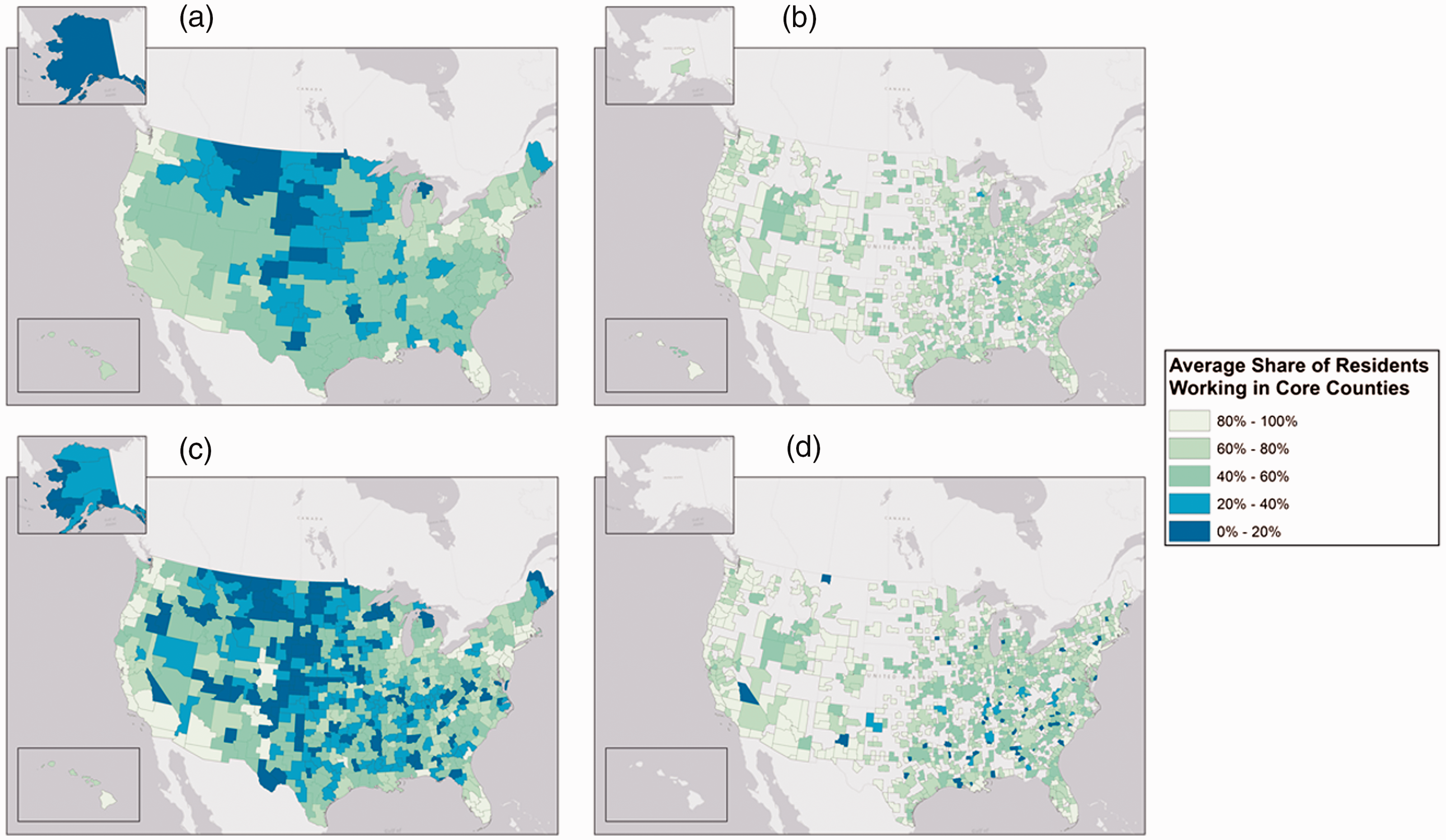
Core—average share of workforce employed in a core county in the labor market. (a) BEA Economic Areas; (b) OMB CBSA's; (c) ERS Commuting Zones and (d) Tong and Plane Combined.

Connection measures

The key measure of connection—the economic activity present in a labor market—utilizes the analysis of average pairwise correlation in wages. The results suggest that labor markets generally perform well on this metric (mean correlations are all ≥0.8) and that there is little differentiation across delineations. All of the delineations here have mean correlations of between 0.82 and 0.98. Note that the extremely high performance of the CBSA and Tong and Plane delineations is partially contingent on the large number of single-county labor markets in those delineations. When we examine the average correlations with single-county observations removed (e.g., mean 2+ in Table 4), those delineations perform more in line with the other delineations. Note that the larger BEA labor markets pay a small penalty in average correlation compared to the ERS delineations, but the difference is not large. Moreover, comparison of the delineations using the online mapping tool at https://sites.psu.edu/psucz shows that all of the delineations are picking up a rather similar spatial pattern in the correlations. Given similar results across four different methodologies, it seems reasonable to believe that what is being observed is a difference in how counties are related to each other rather than an artifact of a specific delineation. Another item worth noting is that the spatial autocorrelation in fit is considerably higher for the BEA delineation than for the others. Also, as the minimum labor-market values in Table 4 show, these relatively high averages obscure labor markets with significantly weaker average correlations.

Containment measures

Finally, the key measure of containment—the share of the population that lives and works in the same labor market (“home” in Table 4)—shows a high level of success across all delineations, with the BEA delineations having an edge over the others. With an average of 93% of labor-market residents working in their labor market, the 2010 BEA delineation shows the benefit of using large labor markets as opposed to the smaller ERS CZs and the core-centric CBSA and Tong and Plane delineations. Figure 2 makes this even clearer. Particularly in the eastern half of the USA, overlapping commuting patterns make the smaller core-based and CZ delineations problematic. While the eastern BEA economic areas perform less well than they do in the West, they do not decline in quality as severely as the other delineations.

Figure 2.

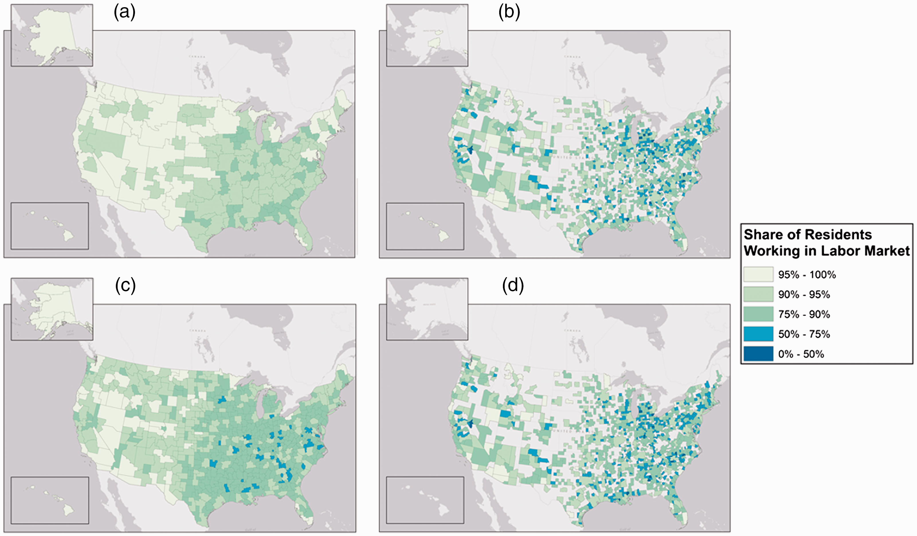
Containment—share of residents working in labor market. (a) BEA Economic Areas; (b) OMB CBSA's; (c) ERS Commuting Zones and (d) Tong and Plane Combined.

Application to specific analyses

We imagine three ways in which researchers might use the heuristics and fit statistics provided in the previous sections. First and most straightforward, we hope this paper will serve as a basic reference to justify the suitability and reasonableness of labor markets as observations in research. We feel that labor markets describe a real geographic phenomenon that, while hard to define precisely, nevertheless captures a context that has meaning for its residents. While there are differences among them, the delineations above perform well on most of our metrics, and the analysis conducted here should provide support for their continued use.

Second, these statistics can be used by researchers to change the labor-market units themselves by modifying the rules for inclusion/exclusion of a county in a labor market. While these delineations are broadly successful, specific research applications may suggest ways in which the delineations might be modified to increase their usefulness. The authors’ own experience in support of federal agencies’ work to define fundamental concepts such as “urban” and “rural” suggest that the 25% commuting threshold employed in the CBSA delineation may be too high for some applications and far too low for others. The county-level statistics provided in conjunction with this paper will allow researchers to customize extant delineations to their own research needs. This may offer a significant improvement over “off the shelf” use of these delineations and can increase the utility of existing delineations without requiring a deep dive into the specifics of how specific delineations were developed.

Third, researchers could use fit statistics to subset a given delineation or weight observations within a delineation based on some relevant measure of quality (e.g., contains a core county, or home containment exceeds 80%). If a research question is only relevant for true labor markets (however defined), then this kind of subsetting or weighting might reduce noise in the analysis and make effects more visible. It may also help as a form of robustness check to determine whether observed results are more or less likely when controlling for imperfect observations. The use of fit statistics can also help detect outliers in the data that arise from peculiarities of the data aggregation, even if these peculiarities do not result in extreme values. Practices such as these are already typical when issues of quality impact other kinds of data, but the complexity of aggregation to geographical units does not excuse researchers from careful understanding of how assumptions shape the outcomes they observe.

The tools and delineations provided at https://sites.psu.edu/psucz allow analysts to use all of the metrics described here, as well as explore visualizations of the variation in metrics within and across delineations. The site includes delineations in comma-delimited and spatial formats for all the years covered in this paper. Separate files are provided for labor markets and counties with labor-market delineations assigned to them. Note that while Tables 3 and 4 focus on summary statistics for each delineation, the provided files have disaggregated statistics for each labor market and, in most cases, for each county within its assigned labor market. These detailed files offer maximum flexibility for researchers seeking to test or customize delineations. The interactive mapping tool on the site also permits researchers to compare basic visualizations of difference easily within and across delineations.

Conclusion

Researchers interested in the study of regional variation have long struggled with getting the units right. For many types of regional analysis, counties will simply be too small or too spatially autocorrelated to be useful, while states may be too large or hide too much internal variation. The concept of the labor market strikes an appropriate balance, but its delineation is not straightforward. In this paper, we have first offered a heuristic for establishing the conceptual basis for employing labor markets as units of observation. This critical first step allows the researcher some clarity in how to choose among extant delineations of labor markets and how these delineations might be modified to approximate the conceptual model more closely. Next, we offered a series of measures that identify variations in the quality of units within delineations and help to differentiate among extant delineations created with very different methodologies. Ultimately, we find that the delineations considered here vary in quality largely consistent with their original intent. The CBSA delineation has advantages over others for analyses focused on core-based labor markets with no metropolitan area split and a high share of the population commuting to core areas. The ERS CZ do a good job of including the entire set of US counties while remaining small enough to retain significant variation across relatively small geographic areas. The BEA regions excel with respect to the containment concept, noticeably outperforming the metropolitan-based measures that intentionally sacrifice containment to focus on strongly connected counties. Notably, the various delineations all perform relatively well when considered in terms of wage correlation, suggesting that the labor-market concept as it is imagined by economists is fairly robust across all delineations.

There are several limitations to the present analyses. As stated previously, changing data-collection methods by the census from 2000 to 2008–2012 fundamentally changed commuter flow data. While we believe the commuter flow data derived from the ACS are less swayed by seasonal trends in work, comparability to previous decennial commuter flow data may be influenced by this change. In addition, changes to the nature of work (e.g., remote work) may limit the ability to capture fully the economic integration of a labor market solely through commuter flow data. The definition of core counties and of metropolitan areas also poses some problems, as there is considerable uncertainty in the assignment of core and metropolitan status related to margins of error in the ACS and census-defined tract boundaries that underlie the OMB definition. Additionally, the changed definitions between 2000 and 2010 create complications for the use of core-based fitness metrics across these delineations.

Finally, beyond the specific applications to labor markets in the US context, the above analysis offers a roadmap for the careful treatment of geographic units of observation. Not all geographic contexts are easy to define, and data are only rarely collected in a way that allows for a perfect apportionment of space into different observations. The example of labor markets makes it clear that a precise conceptual definition of our geographic units is an essential starting point for research that includes contextual measures. Next, having determined what conceptually matters, we need to devise statistics that can help us see where, when, and how well our conceptual model is reflected in the data. It is important to consider how the quality of our measures varies across space and over time. Slight variations in methodology or data can have significant impacts and will become entangled in more meaningful changes in how populations are organized in space. Finally, not all observations are created equal. It is common practice in many disciplines to run robustness checks after removing outliers or on subsets of the data. Once we have fit statistics available to us such as the ones presented here for labor markets, a whole range of techniques opens up, allowing us to examine results as they apply to the most conceptually valid observations or after altering the metrics that justify inclusion of a subunit in a particular observation. Geographic context is often complex, and the mechanisms through which context affects outcomes are equally complicated. If geographic measures are to live up to their full potential, then clear theoretical justification and careful measurement of quality need to be a key part of research moving forward.

Supplemental Material

EPN906154 Supplemental Material - Supplemental material for Bridging the gap between geographic concept and the data we have: The case of labor markets in the USA

Supplemental material, EPN906154 Supplemental Material for Bridging the gap between geographic concept and the data we have: The case of labor markets in the USA by Christopher S Fowler and Leif Jensen in Environment and Planning A: Economy and Space

Footnotes

Declaration of conflicting interests

The author(s) declared no potential conflicts of interest with respect to the research, authorship, and/or publication of this article.

Funding

The author(s) disclosed receipt of the following financial support for the research, authorship and/or publication of this article: This project has been supported by a Cooperative Agreement (No. 58-6000-4-0053) with the Economic Research Service, USDA. We also acknowledge assistance provided by the Population Research Institute at Penn State University, which was supported by an infrastructure grant by the Eunice Kennedy Shriver National Institute of Child Health and Human Development (R24- HD041025). Leif Jensen was supported by a USDA-funded Hatch Multistate Project W-3001, “The Great Recession, Its Aftermath, and Patterns of Rural and Small Town Demographic Change,” administered through Penn State College of Agricultural Sciences Experiment Station Project Number PEN04504.

Notes

ORCID iD

Christopher S Fowler

Supplemental material

Supplemental material for this article is available online.

References

Armington

Acs

(2010) The determinants of regional variation in new firm formation. Regional Studies 36(1): 33–45.

Bureau of Labor Statistics (2019) Quarterly census of employment and wages. Available at: https://www.bls.gov/cew/ (accessed 20 January 2020).

Casado-Diaz

Coombes

(2011) The delineation of 21st century local labour market areas: a critical review and a research agenda. Boletin de la Associacion Geografps Espanoles 57: 7–32.

Casado-Díaz

Martínez-Bernabéu

Flórez-Revuelta

(2016) Automatic parameter tuning for functional regionalization methods. Papers in Regional Science 96(4): 859–880.

Chaix

Méline

Duncan

, et al. (2013) GPS tracking in neighborhood and health studies: a step forward for environmental exposure assessment, a step backward for causal inference? Health and Place 21: 46–51.

Chetty

Hendren

Kline

, et al. (2014) Where is the land of opportunity? The geography of intergenerational mobility in the United States. Quarterly Journal of Economics 129(4): 1553–1623.

Crowder

Krysan

(2016) Moving beyond the big three: a call for new approaches to studying racial residential segregation. City and Community 15(1): 18–22.

Economic Research Service (2015) Commuting zones and labor market areas documentation. Available at: www.ers.usda.gov/data-products/commuting-zones-and-labor-market-%09areas/documentation.aspx (accessed 20 January 2020).

Federal Communications Commission (2010) FCC areas. Available at: https://www.fcc.gov/oet/maps/areas (accessed 20 January 2020).

10.

Foote

Kutzbach

Vilhuber

(2017) Recalculating—how uncertainty in local labor market definitions affects empirical findings. Unpublished manuscript. Available at: https://digitalcommons.ilr.cornell.edu/ldi/45 (accessed 5 February 2020).

11.

Fotheringham

Wong

DWS

(1991) The modifiable areal unit problem in multivariate statistical analysis. Environment and Planning A: Economy and Space 23(7): 1025–1044.

12.

Fowler

Kleit

(2014) The effects of industrial clusters on the poverty rate. Economic Geography 90(2): 129–154.

13.

Fowler

Frey

Folch

, et al. (2019) Who are the people in my neighborhood?: The “contextual fallacy” of measuring individual context with census geographies. Geographical Analysis 1–16. https://doi.org/10.1111/gean.12192

14.

Fowler

Rhubart

Jensen

(2016) Reassessing and revising commuting zones for 2010: history, assessment, and updates for U.S. “labor-sheds” 1990–2010. Population Research and Policy Review 35(2): 263–286.

15.

Gabe

(2006) Growth of creative occupation in U.S. metropolitan areas: a shift-share analysis. Growth and Change 37(3): 396–415.

16.

Galster

(2019) Making our Neighborhoods, Making our Selves. Chicago: University of Chicago Press.

17.

Ganning

Baylis

Lee

(2013) Spread and backwash effects for nonmetropolitan communities in the U.S. Journal of Regional Science 53(3): 464–480.

18.

Garloff

Pohl

Schanne

(2011) Do small labor market entry cohorts reduce unemployment? Available at: https://www.econstor.eu/handle/10419/57468 (accessed 20 January 2020).

19.

Gentleman

Lang

(2007) Statistical analyses and reproducible research. Journal of Computational and Graphical Statistics 16(1): 1–23.

20.

Gibbs

Bernat

(1998) Rural industry clusters raise local earnings. Rural Development Perspectives 12(3): 18–25.

21.

Goodman

JFB

(1970) The definition and analysis of local labour markets: some empirical problems. British Journal of Industrial Relations 8(2): 179–196.

22.

Green

(2009) Labor markets, regional. In: Kitchin

Thrift

(eds) International Encyclopedia of Human Geography. Amsterdam: Elsevier, pp.79–84.

23.

Halás

Klapka

Hurbánek

, et al. (2018) A definition of relevant functional regions for international comparisons: the case of Central Europe. Area 51(3): 489–499.

24.

Halás

Klapka

Tonev

(2016) The use of migration data to define functional regions: the case of the Czech Republic. Applied Geography 76: 98–105.

25.

Hwang

(2015) The social construction of a gentrifying neighborhood: reifying and redefining identity and boundaries in inequality. Urban Affairs Review 52(1): 98–128.

26.

Johnson

Phillips Shively

Stein

(2002) Contextual data and the study of elections and voting behavior: connecting individuals to environments. Electoral Studies 21(2): 219–233.

27.

Johnston

Forrest

Jones

, et al. (2016) The scale of segregation: ancestral groups in Sydney, 2011. Urban Geography 37(7): 985–1008.

28.

Jones

Paasi

(2013) Guest editorial: regional world(s): advancing the geography of regions. Regional Studies 47(1): 1–5.

29.

Killian

Parker

(1991) Higher education no panacea for weak rural economies. Rural Development Perspectives 7(1): 2–7.

30.

Kropp

Schwengler

(2016) Three-step method for delineating functional labour market regions. Regional Studies 50(3): 429–445.

31.

Kwan

(2012) The uncertain geographic context problem. Annals of the Association of American Geographers 102(5): 958–968.

32.

Leventhal

Brooks-Gunn

(2003) Moving to opportunity: an experimental study of neighborhood effects on mental health. American Journal of Public Health 93(9): 1576–1582.

33.

Goodchild

Church

(2013) An efficient measure of compactness for two-dimensional shapes and its application in regionalization problems. International Journal of Geographical Information Science 27(6): 1227–1250.

34.

Logan

Stults

(2014) Interpolating U.S. decennial census tract data from as early as 1970 to 2010: a longitudinal tract database. The Professional Geographer 66(3): 412–420.

35.

Ludwig

Duncan

Gennetian

, et al. (2013) Long-term neighborhood effects on low-income families: evidence from moving to opportunity. American Economic Review 103(3): 226–231.

36.

McKenzie

(2013) County-to-county commuting flows: 2006–2010. Available at: http://www.census.gov/hhes/commuting/ (accessed 20 January 2020).

37.

Marshall

(1890) Principles of Economics. 1st ed. London: Macmillan.

38.

Mas-Colell

Whinston

Green

(1995) Microeconomic Theory. New York: Oxford University Press.

39.

Office of Management and Budget (2010) 2010 Standards for delineating metropolitan and micropolitan statistical areas. Available at: https://www.federalregister.gov/documents/2010/06/28/2010-15605/2010-standards-for-delineating-metropolitan-and-micropolitan-statistical-areas (accessed 20 January 2020), pp. 37245–37252.

40.

Openshaw

Taylor

(1981) The modifiable areal unit problem. In: Wrigley

Bennett

(eds) Quantitative Geography: A British View. London: Routledge, pp.60–69.

41.

Östh

Malmberg

Andersson

(2014) Analysing segregation with individualized neighborhoods defined by population size. In: LLoyd

Shuttleworth

Wong

(eds) Social-Spatial Segregation: Concepts, Processes and Outcomes. Bristol: Policy Press.

42.

Park

Burgess

(1925) The City. Chicago: University of Chicago Press.

43.

Pike

(2011) Placing brands and branding: a socio-spatial biography of Newcastle Brown Ale. Transactions of the Institute of British Geographers 36(2): 206–222.

44.

Plane

(1981) The geography of urban commuting fields: some empirical evidence from new England. Professional Geographer 33(2): 182–188.

45.

Root

Meyer

Emch

(2011) Socioeconomic context and gastroschisis: exploring associations at various geographic scales. Social Science and Medicine 72(4): 625–633.

46.

Sampson

(1997) Neighborhoods and violent crime: a multilevel study of collective efficacy. Science 277(5328): 918–924.

47.

Sampson

(2019) Neighbourhood effects and beyond: explaining the paradoxes of inequality in the changing American metropolis. Urban Studies 56(1): 3–32.

48.

Schroeder

(2007) Target-density weighting interpolation and uncertainty evaluation for temporal analysis of census data. Geographical Analysis 39(3): 311–335.

49.

Smart

(1974) Labour market areas: uses and definition. Progress in Planning 2: 239–353.

50.

Spielman

Folch

(2015) Reducing uncertainty in the American Community Survey through data-driven regionalization. PLoS One 10(2): e0115626.

51.

Tickamyer

Bokemeier

(1987) Sex differences in labor-market experiences. Rural Sociology 53(2): 166–189.

52.

Tong

Plane

(2014) A new spatial optimization perspective on the delineation of metropolitan and micropolitan statistical areas. Geographical Analysis 46(3): 230–249.

53.

United States Census Bureau (2000) Decennial census questionnaires for 1990 and 2000. Available at: https://www.census.gov/dmd/www/2000quest.html (accessed 20 January 2020).

54.

United States Census Bureau (2016) About metropolitan and micropolitan statistical areas. Available at: http://www.census.gov/population/metro/about (accessed 20 January 2020).

55.

United States Census Bureau (2017) Commuting (journey to work). Available at: https://www.census.gov/hhes/commuting/data/commutingflows.html (accessed 20 January 2020).

56.

Van Nuffel

(2007) Determination of the number of significant flows in origin—destination specific analysis: the case of commuting in Flanders. Regional Studies 41(4): 509–524.

57.

Vanheuvelen

(2018) Recovering the missing middle: a mesocomparative analysis of within-group inequality. American Journal of Sociology 123(4): 1064–1116.

58.

Warf

(2017) Spatial turn. In: Turner

(ed) The Wiley-Blackwell Encyclopedia of Social Theory. Oxford: John Wiley, pp.1–3.

59.

Zenk

Schulz

Matthews

, et al. (2011) Activity space environment and dietary and physical activity behaviors: a pilot study. Health and Place 17(5): 1150–1161.

60.

Zipf

(1949) Human Behavior and the Principle of Least Effort. Oxford: Addison-Wesley.

Supplementary Material

Please find the following supplemental material available below.

For Open Access articles published under a Creative Commons License, all supplemental material carries the same license as the article it is associated with.

For non-Open Access articles published, all supplemental material carries a non-exclusive license, and permission requests for re-use of supplemental material or any part of supplemental material shall be sent directly to the copyright owner as specified in the copyright notice associated with the article.

0.00 MB

0.35 MB