A general framework for using the rate law to simulate morphological response to disturbance in the fluvial system

Abstract

A general framework for modelling morphological responses to perturbation is proposed, based on the underpinning principle that the rates of morphological response in alluvial channels are initially high and then decrease through time as the system relaxes following disturbance. The framework includes three morphological response models, each developed from the fundamental rate law, which has the form of an exponential decay function. These models consider the possibility that characteristic behaviours of the fluvial system, such as delayed response and/or cumulative effects, may affect morphological responses, making them capable of representing relaxation paths and times for a range of morphological response variables, whatever their initial states. To test their utility, the models in the framework were applied to simulate the sequence of geomorphological responses to disruption observed in selected rivers with well-documented histories of morphological perturbation, adjustment and recovery. The results demonstrate that the models in the general framework can successfully simulate temporal and spatial patterns of morphological response in the fluvial system under a range of different circumstances, while also indicating how their reliability could be further improved.

Keywords

disturbance fluvial system morphological response rate law relaxation time Colorado River Yellow River

I Background and introduction

There is a rich history of investigation of morphological adjustment in fluvial systems disturbed by, for example, dam construction, channel modification, land-use changes and volcanic eruptions (Kasai, 2006; Leon et al., 2009; Petts and Gurnell, 2005; Rinaldi, 2003; Simon, 1992; Urban and Rhoads, 2003; Williams and Wolman, 1984). Description and prediction of geomorphic responses in the fluvial system should cover four components of channel change: direction, magnitude, time rate and spatial extent (Knighton, 1998). Moreover, a pervasive tendency and significant characteristic of natural, geomorphological systems is for morphological adjustments to lag behind changes in process intensity. This occurs, first, due to the time taken for morphology to begin responding to perturbation, which is referred to as reaction time, and, second, due to the time needed for fluvial processes to perform the work necessary for morphological responses to achieve a balanced state between flow, sediment conveyance and channel form through sediment erosion, transfer and deposition, which is termed the relaxation or recovery time (Brunsden, 1980; Howard, 1982). This explains why models should allow for the existence of reaction and recovery times, which characterize the behaviour of a fluvial system in terms of delayed response and the time necessary for adjustments to fully absorb the effects of disturbance. In nature, reaction and recovery times are characteristically longer than the return period for events that perturb the fluvial system. It follows that the current morphological state of a fluvial system represents the cumulative effects of all previous disturbances and environmental conditions.

Hence, it must be concluded that any comprehensive method or model describing or predicting relaxation paths and times in the fluvial system following disturbance must include the direction, magnitude, rate and extent of geomorphic response. Furthermore, delayed response and/or the cumulative effects of the previous disturbances and conditions, which represent important characteristics of the fluvial system, should also be taken into account when explaining or simulating channel morphologies and adjustments.

Studies by Huang and Nanson (2000, 2002) demonstrated that natural channels adjusted iteratively, with the magnitude of adjustments decaying through time; providing a physical explanation for self-regulatory behaviour in fluvial systems. In this context, the equilibrium condition performs as the attractor state in the evolution of fluvial systems, though it may not necessarily be the actual state that the river achieves once it has relaxed following disturbance (Huang and Nanson, 2000, 2002; Nanson and Huang, 2008). Phillips (2010) argued, however, that the dynamic and variable responses in geomorphology of rivers were just emergent byproducts of fundamental physical mechanisms within them. The steady-state was just a possible state towards which a channel changes, rather than inevitable or normal trends; thus, it should not imply the goal function or attractor state of river evolution. In recognition of multiple potential characteristic or equilibrium forms in the evolution of fluvial systems, Phillips (2009, 2010) indicated that responses or adjustments to imposed changes were finite and therefore they were ultimately characterized by relaxation time equilibrium, the weakest form of equilibrium notions, implying that a stream has completed its response to a given disturbance or environmental change. Therefore, in practice, the equilibrium concept or relaxed state associated with the tendency for responses to disturbance that are dominated by negative feedback mechanisms may be taken as an asymptotic or reference state towards which rivers relax in modelling the evolution of fluvial systems.

Thus far, no general, quantitative model describing the relaxation path and timing of channel adjustment has yet emerged (Knighton, 1998; Leon et al., 2009; Urban and Rhoads, 2003). This is partly explained by the complexity of intrinsic and extrinsic process-response mechanisms in the fluvial system (Hey, 1979), which effectively preclude development of a process-based, deterministic, numerical model capable of simulating morphological responses to disturbance over anything longer than short-term timescales or larger than reach-sized space scales.

As an alternative, a number of conceptual and empirical models have been developed, based on their capability for long-term, system-wide prediction and the relative simplicity of their application. Among these methods, quantitative approaches may be broadly classified as hydraulic geometry analyses, extremal hypotheses and analyses based on various, rational equations.

Hydraulic geometry analyses rely on channel dimensions measured in reaches that are adjusted to the prevailing flow and sediment regimes, which are represented using hydrologic and sediment load records gathered from nearby gauging stations (Hey and Thorne, 1986; Julien and Wargadalam, 1995; Li and Simons, 1982; Millar, 2005; Santos-Cayade and Simons, 1973; Schumm, 1969, 1977; Yu and Wolman, 1987). The resulting equations, usually in the form of power functions (Leopold et al., 1964; Wharton, 1995), can be used to predict the sensitivity of the channel to disturbance and the magnitude and direction of changes in channel dimensions. Most of them, however, apply only to equilibrium conditions and so are incapable of predicting the forms or sequences of transitional geometries displayed by channels that are in disequilibrium as they adjust dynamically to disturbance. In this respect, a conceptual development of regime theory by Hey (1979) sought to account for hydraulic geometry in disequilibrium channels by replacing the flow doing most work through sediment transport with that doing most erosion (in degrading channels) or that doing most deposition (in aggrading channels). While regime-style equations are used extensively and can produce successful outcomes, they suffer several shortcomings (Griffiths, 1984), including the fact that they are not dimensionally homogenous and that their validity is limited to the basin and data from which they were derived.

Extremal hypotheses have been found useful in generating the additional relationships between independent and dependent variables describing fluvial systems necessary for closing the link between fluvial processes, channel adjustment and equilibrium form. The extremal hypothesis may be expressed in terms of minimum stream power per unit bed area, minimum unit stream power per unit weight, minimum flow resistance and maximum sediment transport capacity, etc. (Chang, 1979; Davies and Sutherland, 1983; Kirkby, 1977; Leopold and Langbein, 1962; White and Bettess, 1982; Yalin, 1992; Yang and Song, 1979; Yang et al., 1981). While multiple extremal hypotheses have been proposed, no theory has emerged to unify them and they have been criticized for lacking a basis in Newtonian physics (Huang and Nanson, 2000; Knighton, 1998). Also, satisfaction of an extremal hypothesis strictly applies only in channels that are in equilibrium, which limits their predictive capacity (Qian et al., 1980; Simon and Thorne, 1996).

Rational approaches use power law, hyperbolic and exponential equations or relatively complex differential equations to define and predict river channel changes (Graf, 1977; May, 1976; Simon, 1989; Thorn and Welford, 1994; Williams and Wolman, 1984). A common trait of such models that is widely recognized in nature is that geomorphic systems respond rapidly immediately following disruption, but thereafter exhibit a declining rate of adjustment as a new equilibrium state or a relaxed state is approached (Church, 1995; Knighton, 1998; Simon, 1992; Surian and Rinaldi, 2003; Williams and Wolman, 1984). Consequently, channel response may be described by non-linear decay functions, of which the rate law (an exponential decay function) has been the most widely used to describe relaxation paths and recovery times. For example, Graf (1977) investigated gully development in the Colorado Piedmont and found that growth rates decreased exponentially with time. Soufi (2002) later confirmed this pattern of gully behaviour based on an extensive field survey in Australia. Surian and Rinaldi (2003) and Leon et al. (2009) studied bed level adjustments and transient channel slopes in unstable rivers, respectively, and found that trends in both these variables could be approximated by an exponential function. Many studies have shown that channel response to natural and anthropogenic disturbances (such as those caused by dam construction and channelization) can be simulated and predicted by the rate law, using negative exponential equations (Hooke, 1995; Richard, 2001; Simon, 1989, 1992; Simon and Thorne, 1996; Williams and Wolman, 1984).

Building on the outcomes of these and other studies, Wu and co-workers (Wu et al., 2008a, 2008b) developed a method for predicting changes in bankfull cross-sectional area and bankfull discharge in the Lower Yellow River following closure of dams upstream. They found that predictions based on rate law equations were in good agreement with observed data. Based on the long and largely positive history of application of rate law methods, it is believed that Wu et al.’s methodology can be extended to other rivers and situations where the response time plays a key role in accessing channel adjustment to disturbance or environmental change.

In this paper, we seek to establish, for the first time, a general framework for applying the rate law in a variety of fluvial contexts. This framework builds on and advances the approach developed and reported by Wu et al. (2008a, 2008b). The utility of the proposed framework is tested through application of the equations it contains to simulation of a variety of well-documented geomorphological responses in fluvial systems subject to natural and anthropogenic disruption.

II Theoretical development of the general framework

1 Basic equation

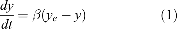
As outlined above, geomorphic adjustment is more intense immediately following disruption, with the rate of change slowing and then becoming asymptotic as a new equilibrium state or a relaxed state is approached. Based on this characteristic of fluvial system, it can be assumed that the rate of adjustment of any morphological variable is proportional to the difference between its value at any time, t, and the asymptotic value toward which it is adjusting. In this respect, Graf (1977) and Knighton (1998) showed that the relaxation path can be described by the following differential equation:

\frac{d y}{d t} = β (y_{e} - y)

where y = a characteristic parameter of fluvial system, y _e = the asymptotic value of this parameter, β = the decay rate that quantifies how rapidly y approaches y _e, and t = time since disturbance.

The relaxation path corresponding to equation (1) following a step-change in a single control variable is shown in Figure 1, which is modified from a graph proposed by Graf (1977). A step-change type of disturbance results from a change to a control variable that is sustained at its new level. Equation (1) and Figure 1 show that, given sufficient time and provided there is no further disturbance, the fluvial system is predicted to adjust to a new equilibrium or relaxed state, y _e, which reflects the self-regulating behaviour that is the characteristic of a fluvial system that was in dynamic equilibrium prior to disturbance. If the reaction time is short, it may be neglected, and Figure 1a can be simplified as Figure 1b.

Figure 1.

Morphological response to step-change in a control variable (dashed line) (a) with a reaction time and (b) without reaction time (solid line indicates the mean condition while dotted line represents short-term fluctuations).

The abrupt step-change in Figure 1 implies a simple, instantaneous change in the controlling variable, which is one of the simplest representations of regime change that can be devised. Presenting the more complicated disturbances encountered in nature, Figure 2, also modified from Graf (1977), illustrates three, typical patterns of step-change observed in nature and the corresponding trends of channel response.

Figure 2.

Schematic representations of morphological responses to different patterns of step-change in a controlling variable.

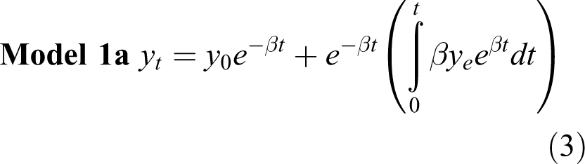
2 Model 1 – basic model

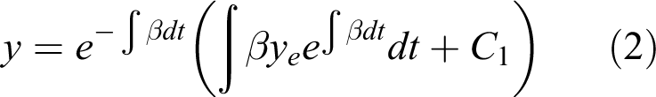
Equation (1) is a first-order ordinary differential equation, and its general solution can be expressed by:

y = e^{- \vint β d t} (\vint β y_{e} e^{\vint β d t} d t + C_{1})

where C₁ = the constant of integration. Using the initial condition that,

y_{0}

, is the initial value of y at t = 0 in equation (2), we can get the first model in the framework:

M o d e l 1 a y_{t} = y_{0} e^{- β t} + e^{- β t} (v i n t l i m i t s_{0}^{t} β y_{e} e^{β t} d t)

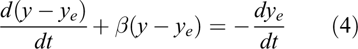
Alternatively, equation (1) can be rewritten in the form:

\frac{d (y - y_{e})}{d t} + β (y - y_{e}) = - \frac{d y_{e}}{d t}

whose general solution is:

y - y_{e} = e^{- \vint β d t} (\vint - \frac{d y_{e}}{d t} e^{\vint β d t} d t + C_{2})

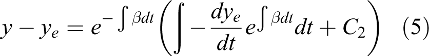
where C₂ = the constant of integration. Similarly, using the initial condition that $y_{0}$ is the initial value of y at t = 0 in equation (5) results in:

\begin{aligned} M o d e l 1 b y_{t} = y_{e} + (y_{0} - y_{e 0}) \\ e^{- β t} - e^{- β t} (v i n t l i m i t s_{0}^{t} e^{β t} \frac{d y_{e}}{d t} d t) \end{aligned}

Equations (3) and (6) are general solutions of the basic equation (equation 1) and are applicable both to simple step-changes (illustrated in Figure 1) and to more complicated cases with more complex disturbances, such as those illustrated in Figure 2. It is straightforward to prove mathematically that these two solutions are equivalent and either one can be applied, depending on how the integration term is to be solved.

3 Model 2 – single-step analytical model

It was noted that dynamical behaviour of the fluvial system means that the asymptotic value of y, $y_{e}$ , may be impossible to predict deterministically because it varies through time. Nevertheless, $y_{e}$ must be known in order to calculate the integration term in either equation (3) or (6). Thus, two simplifying assumptions were adopted here: (1) $y_{e}$ = a constant or (2) $y_{e}$ changes linearly.

If $y_{e}$ is constant, equations (3) and (6) can be simplified as:

M o d e l 2 a y_{t} = (1 - e^{- β t}) y_{e} + e^{- β t} y_{0}

Equation (7) indicates that the value of the morphological variable y is the sum of the weighted initial value $e^{- β t} y_{0}$ and the weighted asymptotic value $(1 - e^{- β t}) y_{e}$ . When $t = 0$ , $y = y_{0}$ and the weighted coefficient for $y_{e}$ is 0. As time passes and the system relaxes towards its asymptotic value, the weight factor for $y_{e}$ (that is 1– $e^{- β t}$ ) increases, while that for $y_{0}$ (that is $e^{- β t}$ ) decreases. This demonstrates how the influence of $y_{e}$ grows while that of $y_{0}$ diminishes, as the system approaches the relaxed state. Finally, as t tends to infinity (that is the time elapsed since disturbance is sufficient for the system to relax), $e^{- β t}$ tends to 0 and $y$ tends to $y_{e}$ .

Alternatively, for the case where $y_{e}$ changes linearly, $d y_{e} / d t = c o n s t$ , integration of either equation (3) or (6) produces:

\begin{aligned} M o d e l 2 b y_{t} = y_{e t} (y_{0} - y_{e 0}) e^{- β t} \\ + (y_{e 0} - y_{e t}) \frac{1}{β t} (1 - e^{- β t}) \end{aligned}

where $y_{e 0}$ and $y_{e t}$ = the potential asymptotic values at the initial time and at time t, respectively.

Model 2 contains just one time period, t, and so may be termed a single-step, analytical model. The two versions differ in that Model 2a is applicable to cases with a constant relaxed state, such as that illustrated in Figure 1, while Model 2b is applicable in cases where the potential relaxed state changes as a linear function of time since disturbance, due to dynamical behaviour of the fluvial system.

4 Model 3 – multi-step analytical model

In a disturbed, alluvial river, the potential relaxed state towards which the system evolves varies as a function of the type and complexity of the disturbance, the time since disturbance, and the recovery path being followed. However, if we divide the relaxation time into a series of short time steps within which y_e can be assumed to be constant, Model 2a can be applied within each time step.

Given that each time step, $Δ t$ , has the same duration, and based on equation (7), after the first time step y can be calculated by:

y_{1} = (1 - e^{- β Δ t}) y_{e 1} + e^{- β Δ t} y_{0}

where the subscript 1 represents the first time step. Similarly, for the second time step:

y_{2} = (1 - e^{- β Δ t}) y_{e 2} + e^{- β Δ t} y_{1}

Substituting equation (9) into equation (10) produces:

y_{2} = (1 - e^{- β Δ t}) [y_{e 2} + e^{- β Δ t} y_{e 1}] + e^{- 2 β Δ t} y_{0}

This procedure is continued to the n^th time step to expand Model 2a (the single-step, analytical model) into a multi-step, analytical model with the form:

\begin{aligned} M o d e l 3 a y_{n} = (1 - e^{- β Δ t}) \sum_{i = 1}^{n} \\ (e^{- (n - i) β Δ t} y_{e i}) + e^{- n β Δ t} y_{0} \end{aligned}

where $y_{n}$ = y, is the value for the n^th time step, n = number of time steps, and $y_{e i}$ = asymptotic value during the i^th time step.

Equation (12) demonstrates the dependency of y on the initial channel condition, $y_{0}$ , which in many cases is unknown. Hence, the applicability of Model 3a could be widened if $y_{0}$ were eliminated or replaced. Theoretically, provided that $e^{- n β Δ t}$ has a value much smaller than unity, the effect of $y_{0}$ on $y_{n}$ gradually diminishes as time proceeds. Thus, $y_{0}$ may be approximated by $y_{e 0}$ , resulting in:

\begin{aligned} M o d e l 3 b y_{n} = (1 - e^{- β Δ t}) \sum_{i = 1}^{n} \\ (e^{- (n - i) β Δ t} y_{e i}) + e^{- n β Δ t} y_{e 0} \end{aligned}

In Model 3, the asymptotic value can vary between time steps to reflect the impact of non-linear, dynamical behaviour in the fluvial system in changing the relaxed condition towards which the channel is adjusting. Consequently, Model 3 is applicable to systems where the relaxed state varies as a complex function of time since disturbance and can account for two important characteristics of natural, fluvial systems: delayed response and the cumulative effects of past disturbances, changing catchment controls and antecedent environmental conditions.

III Applications of the general framework

1 Application of Model 1

As mentioned above, versions 1a and 1b of Model 1 are equivalent, differing only in the way in which their integration terms are composed. Hence, the application of either version of Model 1 should indicate that of the other. In this application, Model 1a was selected to simulate the accumulation of sediment in the main stem of the Yellow River and its largest tributary, the Wei River, following closure of Sanmenxia Dam in 1960.

Sanmenxia Dam is the first dam built on the Yellow River main stem, which carries the highest sediment concentration of all the world’s rivers (Qian and Dai, 1980; Wu and Wang, 2004). The heavy sediment load, together with the initial operating scheme, which made no provision for routing or flushing sediment through the reservoir, led to trapping of all the incoming sediment, resulting in a rapid reduction in its capacity and upstream extension of the backwater zone. Modifications were made to the dam between 1964 and 1973 to increase its capacity to discharge sediment with the aim of achieving a balance between sediment inflow and outflow. Consequently, disturbance and recovery in the fluvial system upstream are characterized by complex morphological responses to raising the base level of the river upstream of Sanmenxia Dam (Wang et al., 2005, 2007; Wu et al., 2007).

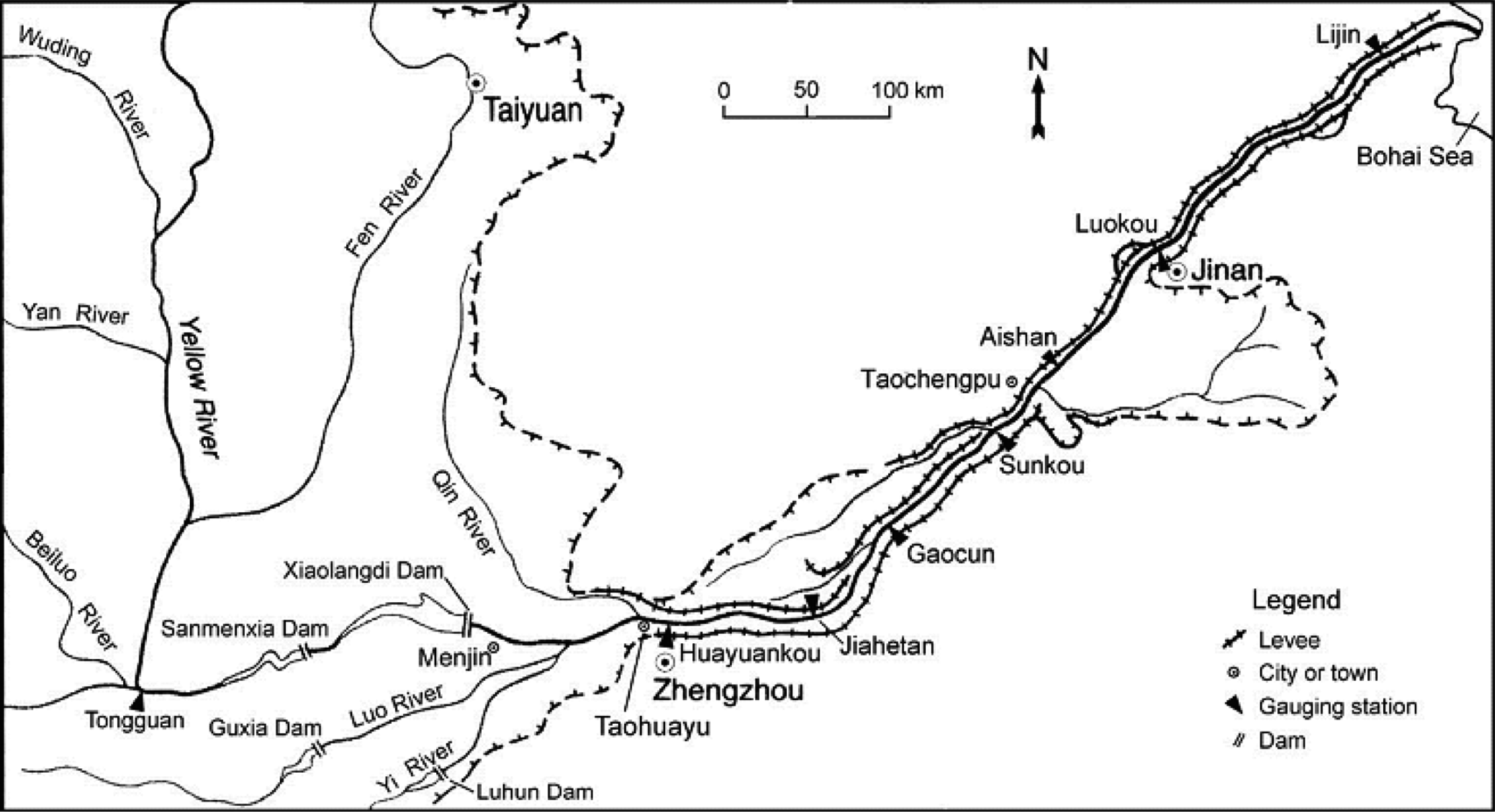
In characterizing temporal changes in base level, the water surface elevation corresponding to a discharge, Q, equal to 1000 m³/s, gauged at the Tongguan hydrometric station, which is located immediately downstream of the confluence of the Yellow and Wei Rivers (Figure 3), was used as a simple but reliable reference value. This reference elevation is termed the ‘river elevation at Tongguan, $Z_{t}$ ’ throughout the following account and its variation following impoundment, dam reconstruction and modification to the flow and sediment regimes is shown in Figure 4.

Figure 3.

Location map of the Yellow River basin.

Figure 4.

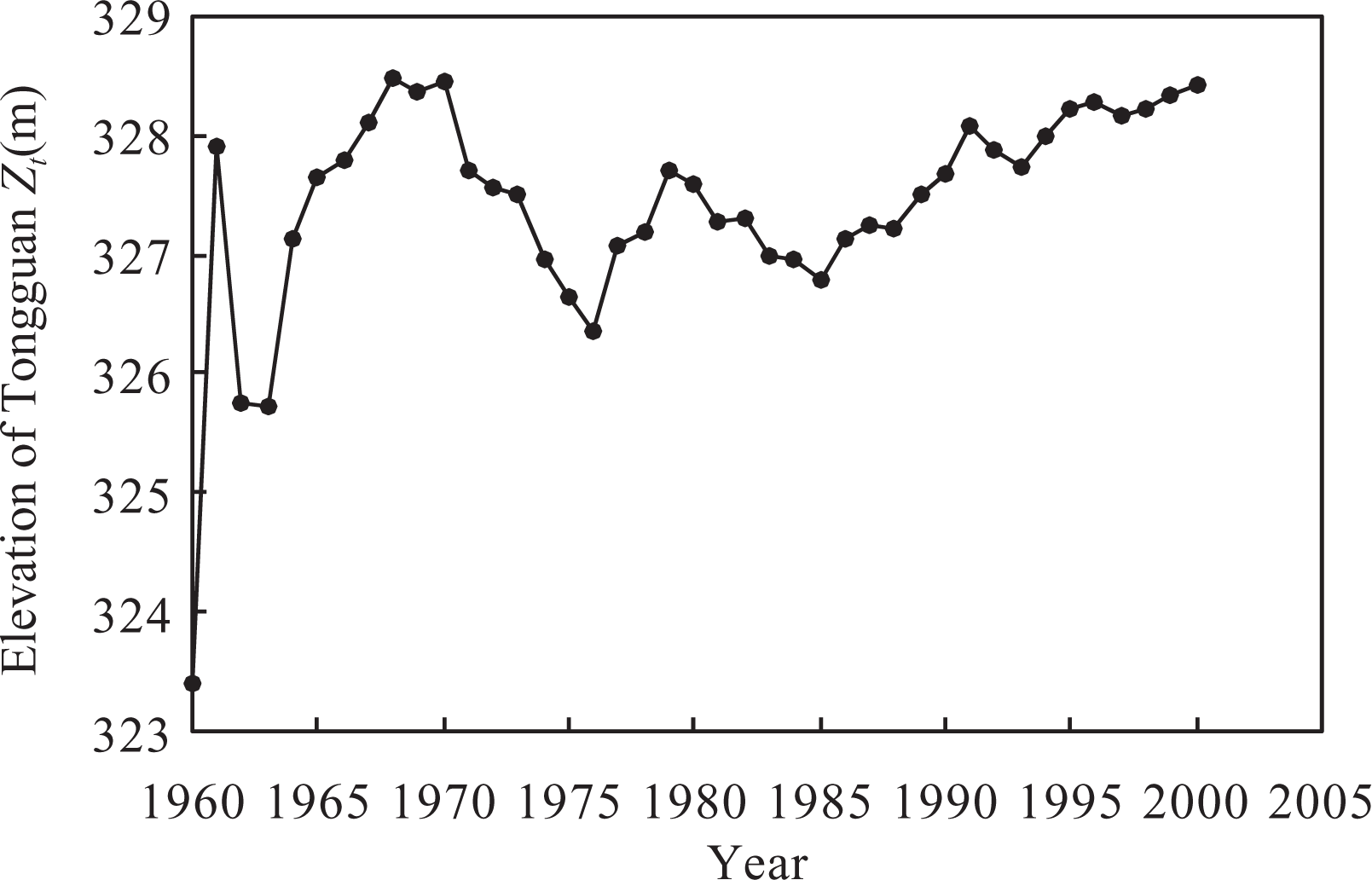
Temporal variation in the river elevation at Tongguan.

Based on Model 1a, the volume of sediment accumulation in the main stem of Yellow River between Longmen and Tongguan (which is known as the Xiaobeiganliu reach) and the lower reaches of the Wei River, V_t (billion m³) can be calculated from:

V_{t} = V_{0} e^{- β t} + e^{- β t} v i n t l i m i t s_{0}^{t} β V_{- .2 p c e} e^{β t} d t

where $V_{0} = 0$ in 1960 when the dam was closed, and t = time elapsed since 1960. The asymptotic value of the volume of the wedge-shaped deposit of accumulated sediment in the reach, V _e, is a geometric function of the increase in the river elevation at Tongguan. According to Wang et al. (2007), it may be calculated by:

V_{e} = A Δ Z_{t} / 2

where $A$ = representative bed area of the accumulated sediment wedge (m²), $Δ Z_{t}$ = net rise in river elevation at Tongguan (m), and $Δ Z_{t} = Z_{t} - Z_{0}$ , where $Z_{t}$ = river elevation at Tongguan at time t (m) and Z₀ = 323.4 m in 1960.

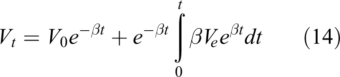
Substituting equation (15) into equation (14) yields:

V_{t} = 0.5 A e^{- β t} (v i n t l i m i t s_{0}^{t} β Δ Z_{t} e^{β t} d t)

The discrete format of equation (16) can be written as:

V_{n} = 0.5 A e^{- β (n Δ t)} (\sum_{i = 1}^{n} β Δ Z_{t i} e^{β (i Δ t)} Δ t)

16a

where $V_{n}$ = volume of accumulated sediment at the end of the n^th time step (billion m³), n = number of time steps or years elapsed since 1960, and $Δ t$ = 1 year.

Solving equation (16) or equation (16a) requires that appropriate values of $A$ and $β$ are specified. These were determined by non-linear regression analysis of field data from the Xiaobeiganliu reach and the lower Wei River between 1960 and 2001, and were found to be:

A = 1.05×10⁹ m², $β = 0.11 / y r .$ (for Xiaobeiganliu reach)

A = 0.53×10⁹ m², $β = 0.13 / y r .$ (for lower Wei River)

The results of solving equation (16a) for the study reaches of the Yellow and Wei Rivers between 1960 and 2001 are presented in Figures 5 and 6. Visual comparison of calculated and observed values in Figure 5 indicates that Model 1a is able to simulate the oscillating and upward trend observed in the volumes of sediment accumulating in the Yellow and Wei Rivers quite well. Figure 6 illustrates the close agreement obtained between observed sediment volumes and those calculated using equation (16a), with the best fit lines explaining 97% and 96% of the variation in observed volume for (a) the Xiaobeiganliu reach and (b) lower Wei River, respectively.

Figure 5.

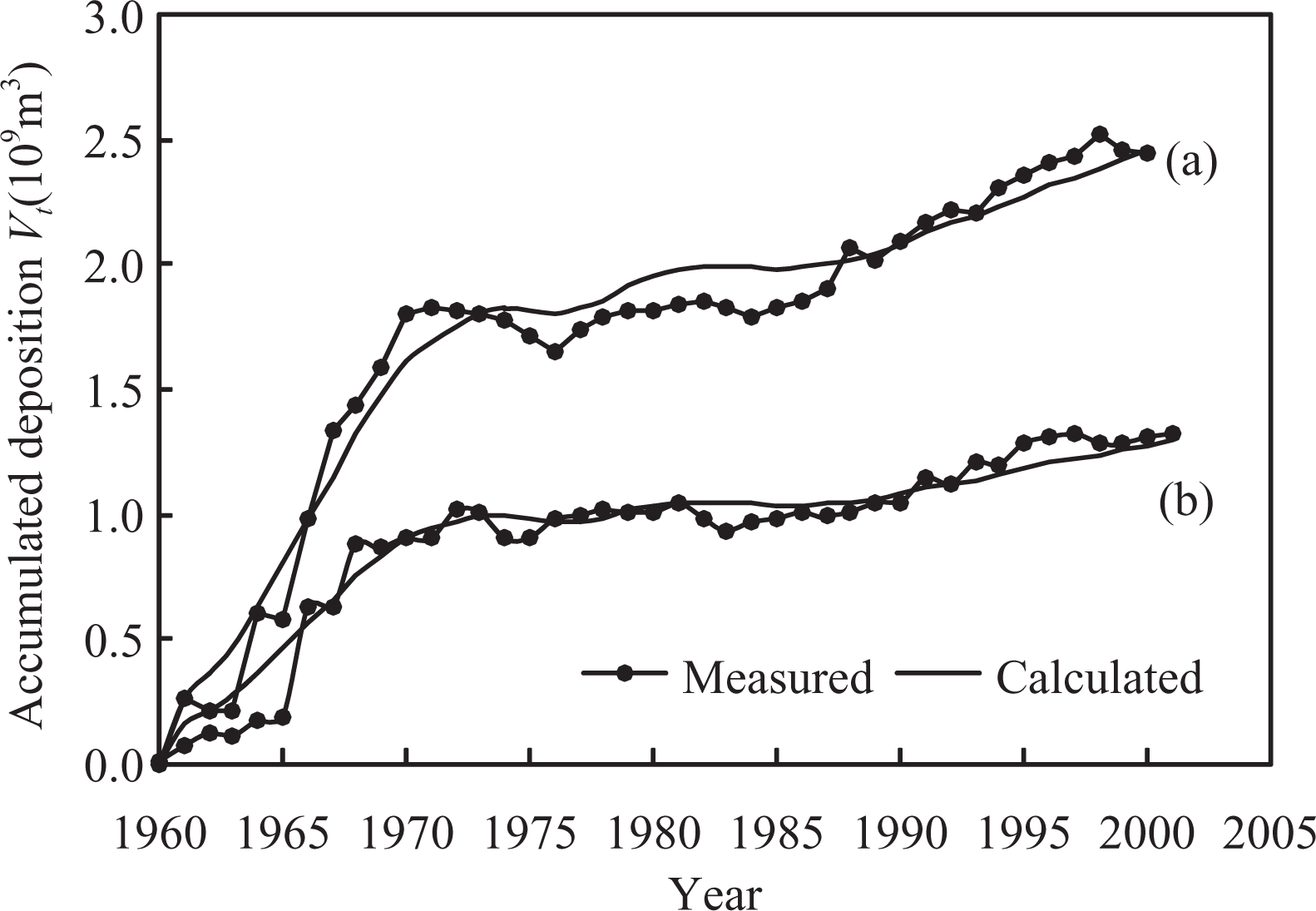
Volume of accumulated sediment observed and computed using Model 1a for (a) the Xiaobeiganliu reach of the Yellow River and (b) the lowest reach of the Wei River.

Figure 6.

Comparison of observed and calculated volumes of sediment accumulation in (a) the Xiaobeiganliu reach and (b) the lower Wei River (R² = coefficient of determination and MSD = mean square deviation).

2 Application of Model 2

Model 2a assumes the relaxed state to be constant, while Model 2b assumes that it changes as a linear function of time since disturbance. Actually, the proclivity of fluvial systems to display complex response limits the frequency of situations where a linear change in the relaxed state is likely to occur. Hence, in this study, a suitable example with which to test Model 2b could not be found. However, no matter how the relaxed state may change, it can be simulated if the user divides the recovery period into a series of time steps, each of which is sufficiently short that the potential relaxed state may be assumed to be constant within each time step, so that Model 2a can be applied on a step-by-step basis. In this approach, the adjustment result for each time step provides the initial condition for the next, so that progressive change in the physical variable can be simulated over the recovery period.

Moreover, as mentioned previously, Model 2a is also applicable to cases with a constant relaxed state, where the system is disturbed by transient changes in a controlling variable. Thus, in this study, Model 2a was applied in cases with both constant and variable relaxed states.

a Response of the Colorado River to dam closure

The Hoover and Davis Dams were built on the Colorado River in 1935 and 1948, respectively. As both dams impound large reservoirs with very high trap efficiencies, the reaches downstream have been starved of sediment since closure of these structures and the relatively clear water released from the dams has eroded the channel bed. In this application, construction of the dams was taken to be a transient disruption and the consequent morphological adjustment of channel bed elevation of the Colorado River was simulated using Model 2a.

Data describing mean bed degradation, $Δ Z_{t}$ , at a cross-section located 9.7 km downstream of Hoover Dam between 1935 and 1948, were obtained from Williams and Wolman (1984). As the elevation of the channel bed at this location in 1935 had not yet been affected by closure of the dam, the initial value, $Δ Z_{0}$ , was set to zero. According to Model 2a, $Δ Z_{t}$ is then related to the asymptotic value of the bed degradation, $Δ Z_{e}$ , and the decay rate $β$ , which were found from regression analysis to be –4.7 m and 0.28/year, respectively. Thus, the equation for $Δ Z_{t}$ at this cross-section can be expressed as follows:

Δ Z_{t} = - 4.7 (1 - e^{- 0.28 t})

The asymptotic value of bed degradation, $Δ Z_{e}$ , is negative (–4.7 m), which represents channel incision.

Similarly, for a cross-section 1.1 km downstream of Davis Dam, the initial value of bed degradation is zero, while $Δ Z_{e}$ and the decay rate $β$ were found to be –5.7 m and 0.17/year, respectively, by regression analysis of data collected between 1948 and 1975. Hence, the calculation equation for reduction of mean channel bed elevation at this cross-section is given by:

Δ Z_{t} = - 5.7 (1 - e^{- 0.17 t})

Figure 7 shows the curves based on solution of equations (17) and (18). Good agreement between the computed and measured channel bed degradation is apparent and the coefficients of determination are 0.97 and 0.98 for the cross-sections downstream of Hoover and Davis Dams, respectively. Moreover, Figure 7 illustrates that the rate of bed degradation was initially rapid but that it gradually diminished to the point that, towards the end of the period of record, there was no obvious change in bed elevation which appeared to be fluctuating around a constant value. This may be taken to indicate relaxation to a graded condition approximating to dynamic equilibrium, at least in terms of the channel long profile.

Figure 7.

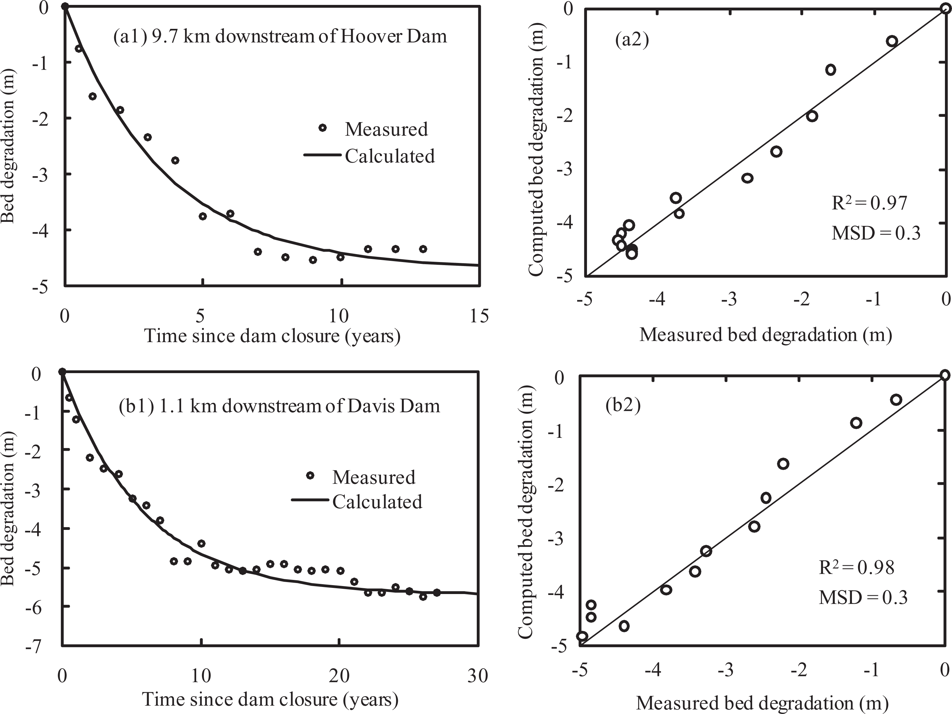
Response of the channel bed elevation to disruption due to dam closure on Colorado River at: (a) a cross-section 9.7 km downstream of Hoover Dam; (b) a cross-section 1.1 km downstream of Davis Dam.

b Reservoir sedimentation and morphological changes in the Yellow River

To test the applicability of Model 2a in a situation with a variable relaxed state, as illustrated above, Model 2a was applied to simulate relaxation paths for (1) reservoir sedimentation behind Sanmenxia Dam, (2) increases in river elevation at Tongguan hydrometric station, and (3) changes in the bankfull dimensions observed at two cross-sections in the Lower Yellow River.

(1) Sedimentation in Sanmenxia Reservoir. When tested, Model 1a was used to simulate sediment accumulation in reaches of Yellow and Wei Rivers affected by backwater effects upstream of the reservoir behind Sanmenxia Dam. This subsection reports the outcome of using Model 2a to simulate sediment deposition in the reservoir between Tongguan and the dam.

Application of Model 2a in situations with a variable relaxed state requires derivation of an equation to calculate the asymptotic value of a morphological parameter closely related to the nature of disruption to the fluvial system. Thus, the first step in applying Model 2a is to identify those physical parameters that primarily responsible for driving morphological response to the particular disturbance being simulated. Then, equations suitable for calculating asymptotic values of the morphological parameters responding to these variables may be developed.

Research by Wu et al. (2007) showed that the discharge flowing into the reservoir and the pool level are the two variables primarily responsible for driving sedimentation in Sanmenxia reservoir. They showed that, consequently, the discharge weighted, average pool level, ${\hat{Z}}_{d}$ (m), could be used to represent the combined effects of discharge Q and pool level $Z_{d}$ on sediment accumulation in the reservoir and this parameter was selected for use in this simulation. The governing equation is:

{\hat{Z}}_{d} = \frac{\sum [Q^{1.5} Z_{d}]}{\sum Q^{1.5}}

The asymptotic value for the volume of sediment accumulated in the reservoir, $V_{e}$ , may be expressed as a function of ${\hat{Z}}_{d}^{}$ using:

V_{e} = K {\hat{Z}}_{d}^{b} + V_{*}

where $V_{*}$ = a characteristic parameter (billion m³), $K$ = a coefficient, and $b$ = an exponent.

Substituting equation (20) into Model 2a (equation 7) produces:

V_{t} = (1 - e^{- β Δ t}) (K {\hat{Z}}_{d}^{b} + V_{*}) + e^{- β Δ t} V_{0}

where V_t and V ₀ = the volume of accumulated sediment at time t and its initial value of the time step, respectively (billion m³), and $Δ t$ = 1 year.

During the first few years after closure, sedimentation is believed to be less strongly related to the operational mode and pool level than is the case in later years. Thus, data for the period 1960–1968 were not used in this study. Furthermore, the operational regime changed from 1974 onwards to ‘storing the clear water and releasing the muddy water’. To reflect this, the time-series data were divided into two periods: 1969–1975 and 1976–2001.

Based on records for these two periods, the coefficients in equation (21) were determined, using non-linear regression analysis, to be:

K = 0.05, b = 1.0, $β$ = 0.6/yr, $V_{*}$ = –12.3 billion m³ (for 1969–1975)

K = 0. 08, b = 1.0, $β$ = 0.6/yr, $V_{*}$ = –21.7 billion m³ (for 1976–2001)

Observed sedimentation volumes in Sanmenxia reservoir are compared to the values calculated using equation (21) in Figure 8(a). The coefficient of determination R² = 0.85.

Figure 8.

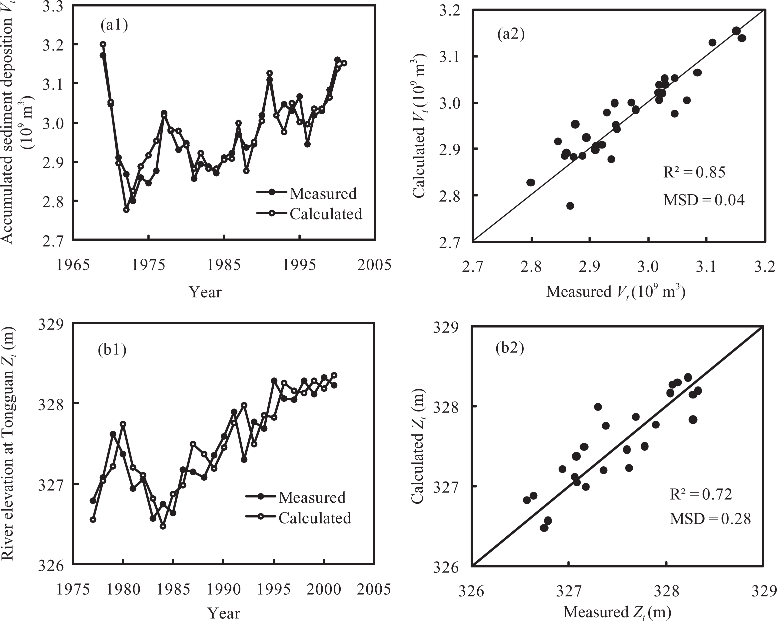
Relaxation paths calculated using Model 2a with a variable relaxed state. (a) Accumulated volume of sediment deposition in the reservoir behind Sanmenxia Dam. (b) River elevation at Tongguan.

(2) Aggradation at Tongguan. As mentioned earlier, the elevation of the Yellow River at Tongguan represents the base level for the reaches of both the Yellow and Wei Rivers upstream. The river elevation at Tongguan is, in turn, strongly affected by sedimentation in the reservoir. In this application, Model 2a is applied to simulate the response of river elevation at Tongguan to post-1975 operation of Sanmenxia Dam.

The asymptotic value of river elevation at Tongguan, $Z_{e}$ , is not constant but varies as a function of the volume of water that flows into the reservoir annually (Wu et al., 2004, 2007). This may be expressed by:

Z_{e} = K W_{a}^{b} + Z_{*}

where $W_{a}$ = annual runoff passing Tongguan station (billion m³), $Z_{*}$ = characteristic parameter of river elevation at Tongguan (m), $K$ = a coefficient, and $b$ = an exponent.

According to Model 2a and equation (22), river elevation at Tongguan can be computed using:

Z_{t} = (1 - e^{- β Δ t}) (K W_{a}^{b} + Z_{*}) + e^{- β Δ t} Z_{0}

where Z_t and Z ₀ = the river elevation at Tongguan at time t and its initial value of the time step, respectively (m). And $Δ t$ = 1 year.

The parameters in equation (23) obtained using regression analysis of data for the period 1977 to 2001 were:

K = –0.014, b = 3.2, $β = 0.3 / y r .$ , $Z_{*}$ = 328.5 m

Observed and computed values of the river elevation at Tongguan are shown in Figure 8(b). The coefficient of determination R ² = 0.72.

(3) Bankfull dimensions. Bankfull discharge and area are principal indicators of the capacity of the main channel of the Lower Yellow River to convey flood flows and transport sediment. As a result of increasing impact of human activities, such as water withdrawal for irrigation and municipal uses, dam construction and land-use changes, sedimentation in the main channel has become ever more serious in the Lower Yellow River, which is perched well above its floodplain. As a consequence, bankfull discharge and area of the Lower Yellow River have decreased dramatically during the last half century.

In this case study, Model 2a is applied to simulate changes in bankfull discharge and area of the Lower Yellow River at Lijin and Gaocun hydrometric stations (Figure 9), respectively, based on results published previously by Wu et al. (2008a, 2008b).

Figure 9.

Location map of the Lower Yellow River.

The shape and dimensions of the channel of the lower reaches of the Yellow River are shaped primarily by the incoming flow and sediment load, especially during the flood season. Consequently, the asymptotic value of the bankfull discharge can be expressed as a function of discharge and suspended sediment load by:

Q_{e} = K ξ_{f}^{b} Q_{f}^{c}

where $Q_{f}$ = average flood season discharge (m³/s) and $ξ_{f}$ = incoming sediment coefficient (kg×s /m⁶), defined by:

ξ_{f} = C_{t f} / Q_{f}

where $C_{t f}$ = average suspended sediment concentration (kg/m³), and K, b and c are parameters.

Based on equation (24) and Model 2a, the equation used to calculate bankfull discharge is:

Q_{b t} = K (1 - e^{- β Δ t}) ξ_{f}^{b} Q_{f}^{c} + e^{- β Δ t} Q_{b 0}

where $Q_{b t}$ and $Q_{b 0}$ = bankfull discharge at time t and its initial value of the time step, respectively (m³/s), and $Δ t$ = 1 year.

Data collected at Lijin hydrometric station between 1960 and 2003 were used to support regression analysis to determine the parameters in equation (26). The resulting values were:

K = 348.6, $β$ = 0.431/year, b = –0.15, c = 0.29.

Similarly, the asymptotic bankfull area, $A_{e}$ (m²), should also be a function of the incoming discharge and sediment load during the flood season, expressed as:

A_{e} = K ξ_{f}^{b} Q_{f}^{c}

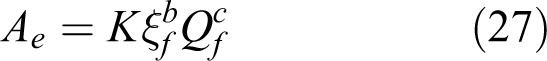
where $ξ_{f}$ and $Q_{f}$ have the same meanings as in equation (24). This leads to the following equation for predicting bankfull area:

A_{b t} = K (1 - e^{- β Δ t}) ξ_{f}^{b} Q_{f}^{c} + e^{- β Δ t} A_{b 0}

where

A_{b t}

and

A_{b 0}

= bankfull area at time t and its initial value of the time step, respectively (m²), and

Δ t

= 1 year.

Using data collected at Gaocun hydrometric station (Figure 9) between 1960 and 2002, the parameter values were found to be:

K = 25.91, $β$ = 0.25/year, b = –0.90, c = 0.10.

Figure 10 compares the observed bankfull discharges and areas to values calculated using equations (26) and (28). The coefficients of determination between measured and computed values of bankfull discharge and area are 0.86 and 0.89, respectively.

Figure 10.

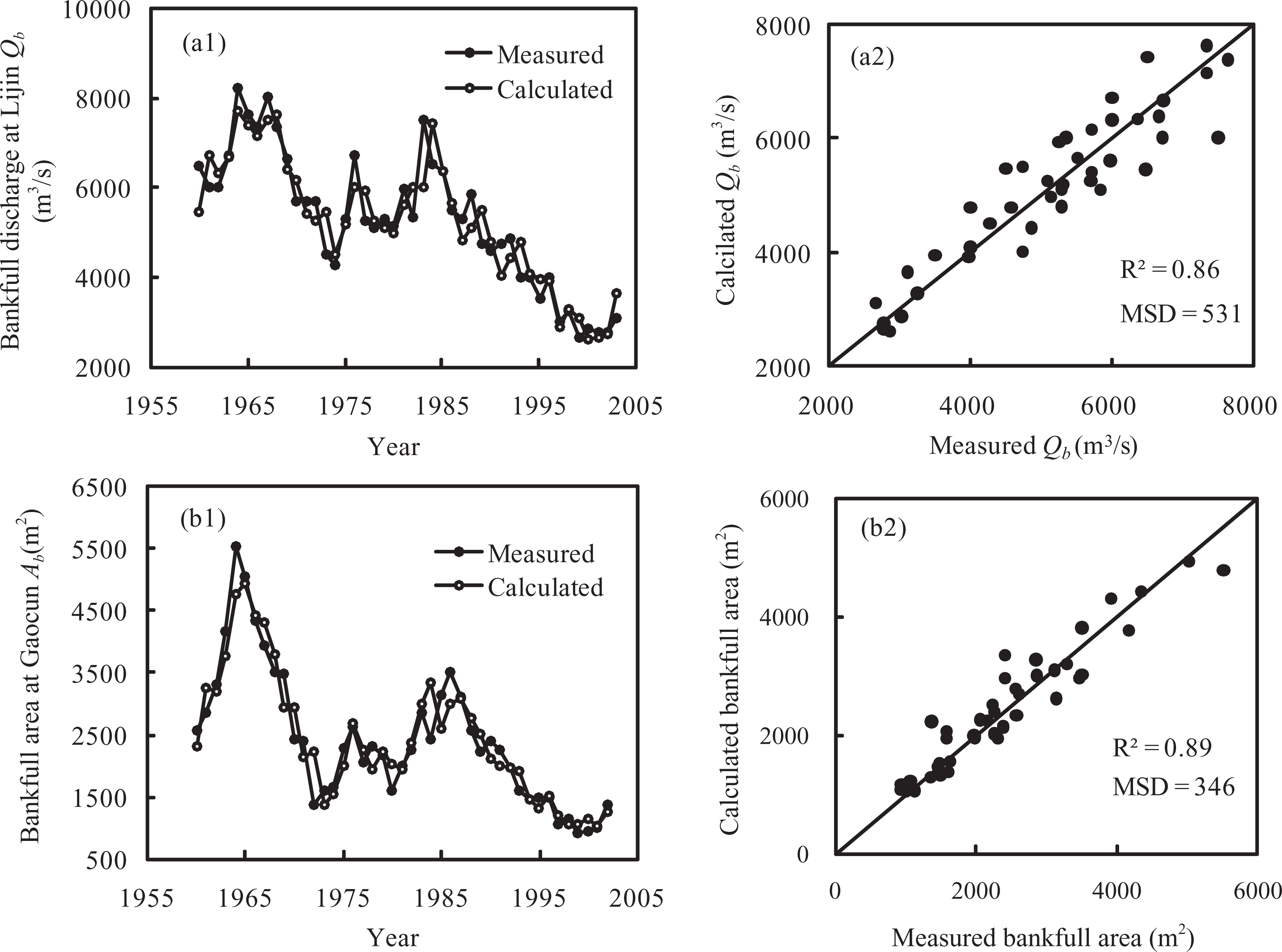
Relaxation paths computed using Model 2a with a variable relaxed state. (a) Bankfull discharge at Lijin station, Lower Yellow River (after Wu et al., 2008a). (b) Bankfull area at Gaocun station, Lower Yellow River (after Wu et al., 2008b).

3 Application of Model 3

There are two versions of Model 3, of which Model 3b may be less reliable than Model 3a because it uses the initial asymptotic value to represent the initial condition in cases where the actual initial condition is unknown. It follows that, if Model 3b can successfully simulate the sequence of adjustments observed in a fluvial system following disturbance, Model 3a would also be able to do so. Consequently, Model 3b was selected for testing through application to the same morphological attributes of the Yellow River that were previously used to test Model 2a (with variable relaxed states). Differences between these two models will be discussed later.

a Sedimentation in Sanmenxia Reservoir

Model 3b was applied to simulate the accumulation of sediment in Sanmenxia reservoir using:

\begin{aligned} V_{n} = (1 - e^{- β Δ t}) \sum_{i = 1}^{n} (e^{- (n - i) β Δ t} V_{e i}) \\ + e^{- n β Δ t} V_{e 0} \end{aligned}

where

V_{n}

= volume of accumulated sediment at the end of the n^th time step (billion m³),

V_{e i}

and

V_{e 0}

= asymptotic values of accumulated sediment at the i^th time step and at the beginning of the relaxation period, respectively (billion m³),

β

= decay rate, and

Δ t

= 1 year.

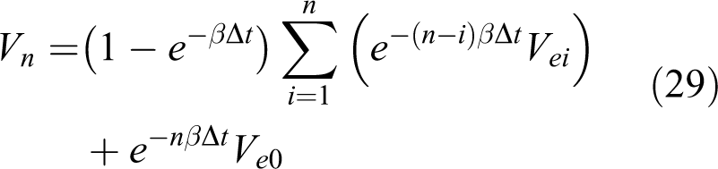
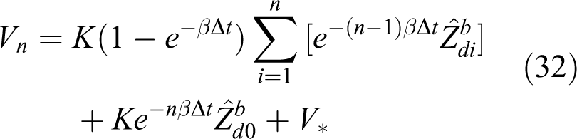
Equation (20), which was used to simulate the asymptotic value of the total sediment deposition volume in the application of Model 2a, was also applied here. Substituting equation (20) into equation (29) results in:

\begin{aligned} V_{n} = (1 - e^{- β Δ t}) \sum_{i = 1}^{n} [e^{- (n - 1) β Δ t} \\ (K {\hat{Z}}_{d i}^{b} + V_{*})] + e^{- n β Δ t} (K {\hat{Z}}_{d 0}^{b} + V_{*}) \end{aligned}

where

{\hat{Z}}_{d i}

and

{\hat{Z}}_{d 0}

= discharge weighted pool level (see equation 19) at the i^th time step and at the initial time t₀ , respectively (m).

The expansion of equation (30) is:

\begin{aligned} V_{n} = K (1 - e^{- β Δ t}) \sum_{i = 1}^{n} [e^{- (n - 1) β Δ t} {\hat{Z}}_{d i}^{b}] \\ + K e^{- n β Δ t} {\hat{Z}}_{d 0}^{b} + V_{*} \{(1 - e^{- β Δ t}) \\ \sum_{i = 1}^{n} [e^{- (n - 1) β Δ t}] + e^{- n β Δ t}\} \end{aligned}

which can be simplified as:

\begin{aligned} V_{n} = K (1 - e^{- β Δ t}) \sum_{i = 1}^{n} [e^{- (n - 1) β Δ t} {\hat{Z}}_{d i}^{b}] \\ + K e^{- n β Δ t} {\hat{Z}}_{d 0}^{b} + V_{*} \end{aligned}

The coefficients in equation (32) were determined from regression analysis of sedimentation data collected between 1969 and 1975, and 1976 and 2001, respectively. The resulting values were:

K = 0.045, $b = 1.0$ , $β = 0.60 / y r .$ , $V_{*} =$ –10.76 billion m³ (for 1969–1975)

K = 0.087, $b = 1.0$ , $β = 0.60 / y r .$ , $V_{*} =$ –23.89 billion m³ (for 1976–2001)

Equation (32) shows that calculated values of sedimentation vary with n, the number of preceding years. To determine the number of preceding years over which conditions affect annual sediment accumulation, coefficients of determination, R² , between measured and computed values were calculated for the period 1969–2001 with n = 1 to 10 years.

R² values increase from 0.65 (for n = 1) to 0.86 (for n = 4), remain constant until n = 8, and then decrease slightly for n = 9 and 10 (Figure 11). This implies that the deposited volume is most closely related to conditions (e.g. incoming discharge and sediment load, pool level adjustment) in the preceding four to five years.

Figure 11.

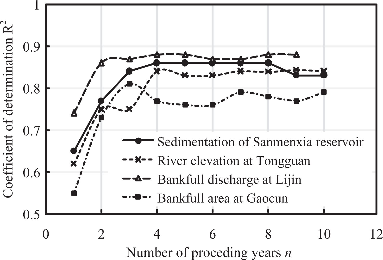
Relationships between coefficient of determination R² and n for four applications.

Observed volumes of accumulated sediment are compared to values calculated using equation (32) (with n = 4 years) in Figure 12(a). Calculated values agree well with the observed values.

Figure 12.

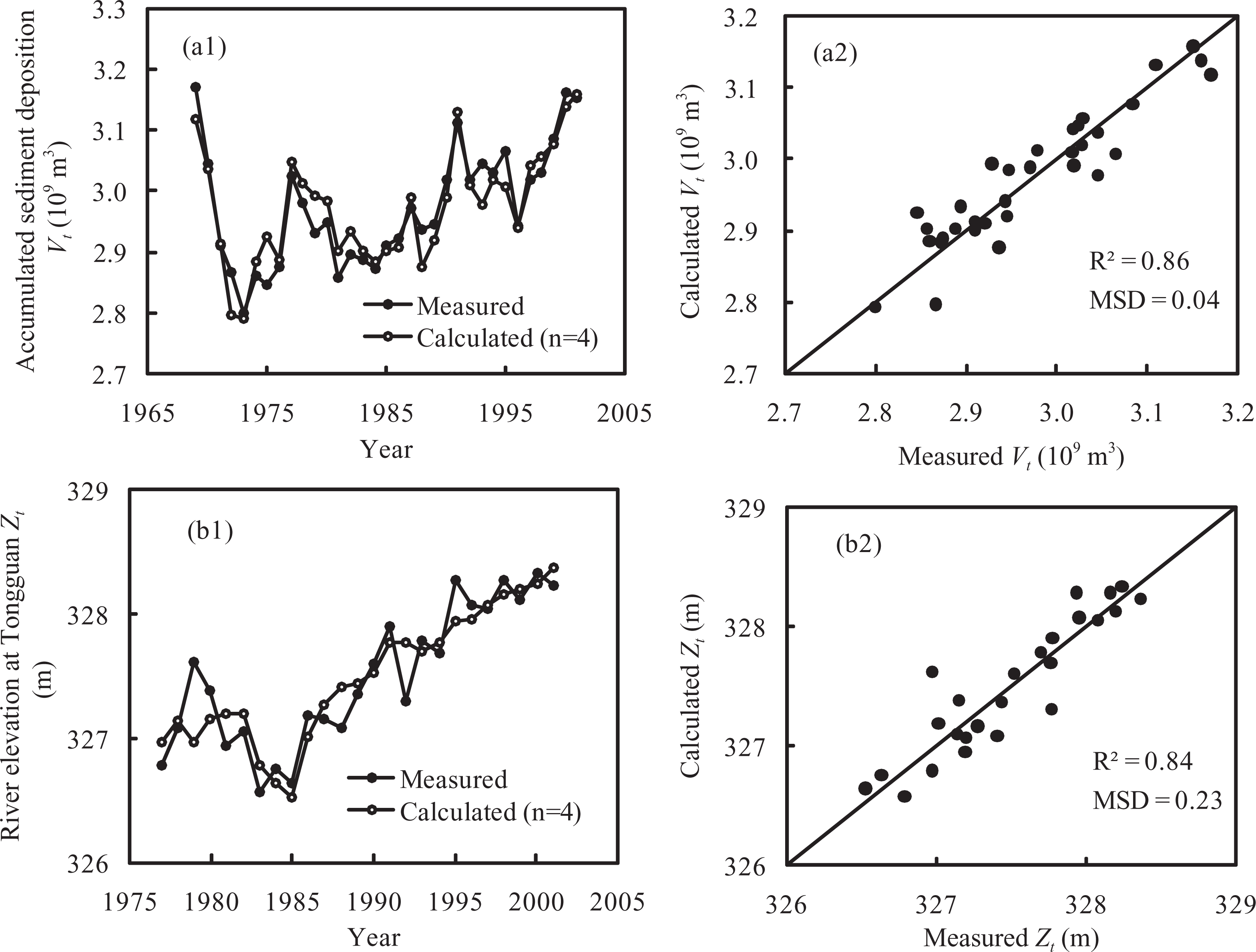
Relaxation paths computed by Model 3b. (a) Accumulated volume of sediment in Sanmenxia reservoir (n = 4). (b) River elevation at Tongguan (n = 4).

b Aggradation at Tongguan

The elevation of the Yellow River at Tongguan, $Z_{n}$ , may be simulated by applying Model 3b using:

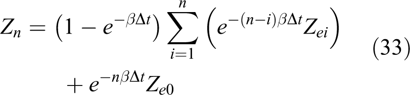
\begin{aligned} Z_{n} = (1 - e^{- β Δ t}) \sum_{i = 1}^{n} (e^{- (n - i) β Δ t} Z_{e i}) \\ + e^{- n β Δ t} Z_{e 0} \end{aligned}

where $Z_{n}$ = river elevation at Tongguan at the end of the n^th time step (m), $Z_{e i}$ and $Z_{e 0}$ = asymptotic values of river elevation at Tongguan at the i^th time step and at the beginning of the relaxation period, respectively (m), $β$ = decay rate, and $Δ t$ = 1 year.

The asymptotic value of river elevation was again calculated using equation (22). Substituting equation (22) for $Z_{e 0}$ and $Z_{e i}$ into equation (33) then produces:

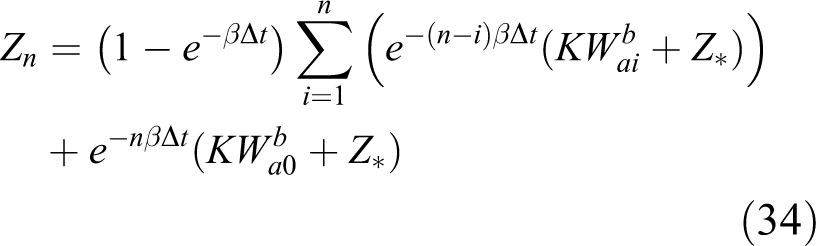
Z_{n} = (1 - e^{- β Δ t}) \sum_{i = 1}^{n} (e^{- (n - i) β Δ t} (K W_{a i}^{b} + Z_{*})) + e^{- n β Δ t} (K W_{a 0}^{b} + Z_{*})

for which the expansion is:

Z_{n} = K (1 - e^{- β Δ t}) \sum_{i = 1}^{n} [(e^{- (n - i) β Δ t} (W_{a i}^{b})] + K e^{- n β Δ t} (W_{a 0}^{b}) + Z_{*} {(1 - e^{- β Δ t}) \sum_{i = 1}^{n} [e^{- (n - i) β Δ t}] + e^{- n β Δ t}}

where $W_{a}$ and W ₀ = annual runoffs passing the Tongguan station at the i^th time step and at the initial time t₀ , respectively (billion m³).

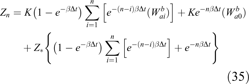
Equation (35) can be simplified as:

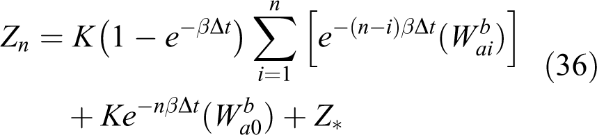
\begin{aligned} Z_{n} = K (1 - e^{- β Δ t}) \sum_{i = 1}^{n} [e^{- (n - i) β Δ t} (W_{a i}^{b})] \\ + K e^{- n β Δ t} (W_{a 0}^{b}) + Z_{*} \end{aligned}

The parameters in equation (36) were found through regression analysis of data collected at Tongguan hydrometric station between 1977 and 2001. The values were:

$K = - 0.0011$ , $b = 2.0$ , $β = 0.40 / y r .$ , Z_* = 328.72 m

The coefficient of determination between computed and observed values for the river elevation at Tongguan rose to 0.84 with increasing values of n until n = 4, but remained constant thereafter (Figure 11). This suggests that river elevation is affected by conditions and channel adjustments during the preceding five years. Observed values are compared to those calculated using equation (36), with n = 4, in Figure 12(b), and good agreement between them can be observed.

c Bankfull dimensions

Model 3b was also applied to simulate changes in bankfull discharge and area of the Lower Yellow River observed at Lijin and Gaocun hydrometric stations, respectively, building on research by Wu et al. (2008a, 2008b).

Using Model 3b, changes in bankfull discharge of the Lower Yellow River can be simulated by:

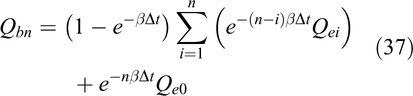
\begin{aligned} Q_{b n} = (1 - e^{- β Δ t}) \sum_{i = 1}^{n} (e^{- (n - i) β Δ t} Q_{e i}) \\ + e^{- n β Δ t} Q_{e 0} \end{aligned}

Substituting the equation for the asymptotic bankfull discharge (equation 24) into equation (37) yields:

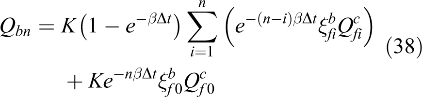
\begin{aligned} Q_{b n} = K (1 - e^{- β Δ t}) \sum_{i = 1}^{n} (e^{- (n - i) β Δ t} ξ_{f i}^{b} Q_{f i}^{c}) \\ + K e^{- n β Δ t} ξ_{f 0}^{b} Q_{f 0}^{c} \end{aligned}

where $Q_{b n}$ = bankfull discharge at the end of the n^th time step (m³/s), $Q_{f i}$ and $Q_{f 0}$ = average discharge during flood season at the i^th time step and at time t₀ (the initial condition), respectively (m³/s), $ξ_{f i}$ and $ξ_{f 0}$ = incoming sediment coefficients at the i^th time step and at time t₀ , respectively (kg×s/m⁶), $β$ = decay rate, and $Δ t$ = 1 year.

Regression analysis of data collected at Lijin hydrometric station between 1960 and 2003 showed that the parameters in equation (38) were very close to those established earlier, in equation (26). Thus, the same set of coefficients was used to predict bankfull discharge at Lijin.

The way that the coefficient of determination between the measured and the computed bankfull discharges (R²) changes with the number of preceding years taken into account (n) was investigated. It was found that R² initially increased with n, but remained constant at about 0.88 for n values higher than four (see Figure 11). Observed values of bankfull discharge are compared to values calculated using equation (38) with n = 4 in Figure 13(a).

Figure 13.

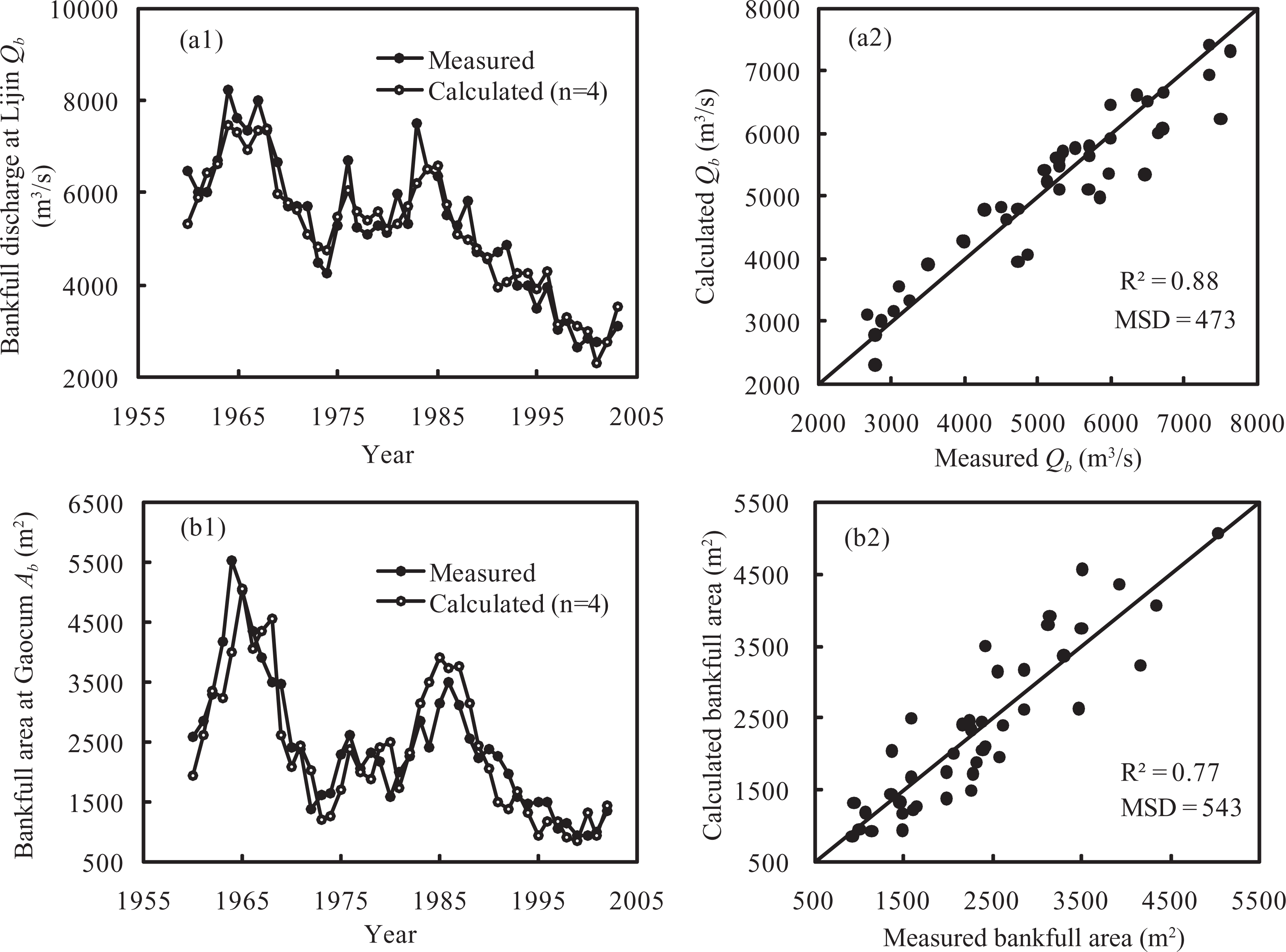
Relaxation paths computed using Model 3b. (a) Bankfull discharge at Lijin (n = 4) (after Wu et al., 2008a). (b) Bankfull area at Gaocun (n = 4) (after Wu et al., 2008b).

Similarly, the equation based on Model 3b for bankfull area at Gaocun station on the Lower Yellow River is:

\begin{aligned} A_{b n} = K (1 - e^{- β Δ t}) \sum_{i = 1}^{n} (e^{- (n - i) β Δ t} ξ_{f i}^{b} Q_{f i}^{c}) \\ + K e^{- n β Δ t} ξ_{f 0}^{b} Q_{f 0}^{c} \end{aligned}

The coefficients calculated earlier for equation (28) were found also to be applicable in equation (39). Variation in A_bn with n was investigated using equation (39). The coefficient of determination between observed and calculated values increased with n, reaching a value close to 0.8 with n = 4, but then remained almost constant. Observed and calculated values of A_bn are compared in Figure 13(b).

The relationships between R² and n revealed by applications of equations (38) and (39) demonstrate that bankfull discharge and dimensions in the Lower Yellow River are influenced by incoming discharges and sediment loads during the preceding four or five years.

IV Discussion and conclusions

A framework for simulating morphological recovery in disturbed fluvial systems has been developed, based on the principle that morphological adjustments occur rapidly immediately after disruption, but that the rate of change decreases with time to become asymptotic as the system relaxes and approaches a new equilibrium or relaxed state. This framework builds on research by Wu et al. (2008a, 2008b) to provide a systematic basis for applying the rate law, which has been widely demonstrated to be capable of accurately describing morphological adjustments in the fluvial system.

The framework includes three different models, each developed from the fundamental rate law equation, which has the form of a negative exponential decay function. The basic model (Model 1) is expressed in two versions that differ only with respect to the integration items. The single-step, analytical model (Model 2) also comes in two versions, which allows the user to select an appropriate assumption concerning how the relaxed state changes as a function of time during the recovery period. Inclusion of two versions of the multi-step, analytical model (Model 3) further allows users to apply advanced rate law modelling even in situations where the initial value of the geomorphological variable under consideration is unknown. These three morphological response models facilitate inclusion of characteristic behaviours of the fluvial system such as delayed response and/or the cumulative effects of antecedent and catchment conditions, which can have different effects on the relaxation times and paths displayed by a variety of morphological variables.

To test the applicability and validity of the proposed framework, Models 1a, 2a and 3b were applied to simulate adjustment of selected morphological variables in rivers following natural or anthropogenic disturbance. Relaxation paths for channel bed elevation, the volume of sediment in aggrading reaches, reservoir sedimentation and bankfull dimensions were calculated and compared to observed data. The results demonstrate that the models in the general framework can successfully simulate relaxation paths for a variety of morphological response variables as they adjust to both impulse and step changes in a controlling variable.

A comparison between Model 2a and Model 3b is provided in Table 1, as both models were used to simulate the morphological adjustment of the Yellow River. There are two main differences between these two models. First, as detailed in Table 1, application of Model 2a requires that initial conditions known (i.e. pre-disturbance values are available for V ₀, Z ₀, Q_b ₀ and A_b ₀). Conversely, initial values are not required to apply Model 3b, as they are replaced by estimated asymptotic values. The second difference lies in how dynamical behaviour of the fluvial system is represented in the models (Figure 14). When applying Model 2a in situations with a variable relaxed state, the value of a variable in each time step is related only to the condition in the preceding time step. However, when applying Model 3b, the number of preceding years over which conditions are considered when calculating a variable’s asymptotic value, n, is optimized by maximizing the coefficient of determination for a regression line fitted to a scatter graph of calculated versus observed values.

Figure 14.

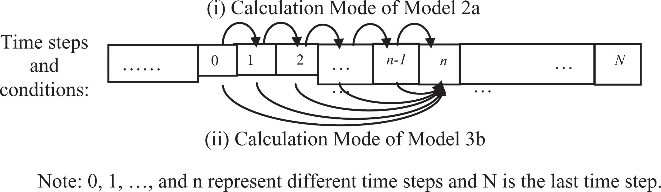
Different calculation modes adopted in applying Models 2a and 3b in cases with a variable relaxed state. (i) Conditions in one time step are taken as the initial conditions for the next time step when applying Model 2a. (ii) Conditions in n preceding time steps (0, 1, … n-1) are taken into the calculation in the n^th time step when applying Model 3b.

Table 1.

Comparison of applications of Models 2a and 3b in the Yellow River

Simulated Variables	Details of models	Model 2a	Model 3b
Accumulated sedimentation volume in Sanmenxia Reservoir	Variables used	V_t , ${\hat{Z}}_{d}$ , V ₀	$V_{n}$ , ${\hat{Z}}_{d i}$ , ${\hat{Z}}_{d 0}$
	Coefficients	$K$ , $β$ , $b$ , $V_{*}$ = 0.05, 0.6, 1, –12.3 (1969–1975); = 0.08, 0.6, 1, –21.7 (1976–2001)	$K$ , $β$ , $b$ , $V_{*}$ = 0.045, 0.6, 1, –10.76 (1969–1975); = 0.087, 0.6, 1, –23.89 (1976–2001)
	Results: R² &MSD	0.85; 0.04	0.86; 0.04 (at n = 4)
River elevation at Tongguan	Variables used	Z_t , W_a , Z ₀	Z_n , W_ai , W_a ₀
	Coefficients	$K$ , $β$ , $b$ , $Z_{*}$ = –0.014, 0.3, 3.2, 328.5	$K$ , $β$ , $b$ , $Z_{*}$ = –0.0011, 0.4, 2, 328.7
	Results: R² &MSD	0.72; 0.28	0.84; 0.23 (at n = 4)
Bankfull discharge at Lijin Station	Variables used	Q_bt , $ξ_{f}$ , Q_f , Q_b ₀	Q_n , $ξ_{f i}$ , Q_fi , $ξ_{f 0}$ , Q_f ₀
	Coefficients	$K$ , $β$ , $b$ , c = 348.6, 0.431, –0.15, 0.29	$K$ , $β$ , $b$ , c = same as Model 2a
	Results: R² &MSD	0. 86; 531	0.88; 473 (at n = 4)
Bankfull area at Gaocun Station	Variables used	A_bt , $ξ_{f}$ , Q_f , A_b ₀	A_n , $ξ_{f i}$ , Q_fi , $ξ_{f 0}$ , Q_f ₀
	Coefficients	$K$ , $β$ , $b$ , c = 25.91, 0.25, –0.9, 0.1	$K$ , $β$ , $b$ , c = same as Model 2a
	Results: R² &MSD	0.89; 346	0.79; 543 (at n = 4)

Furthermore, the findings highlight that good agreement between observed and simulated relaxation paths depends crucially on accurate representation of the decay rate, β, which governs the rate at which a response variable approaches its asymptotic value. In the applications reported herein, β was held constant whereas, in nature, it may vary (Thorne et al., 2010; Wu et al., 2008b). It is suggested that the reliability of the models in the framework could be improved through further research on how dynamical behaviour in the fluvial system affects the decay rate.

The findings also demonstrate the key role that accurate representation of the asymptotic value, towards which the variable is adjusting, plays in successful application of the models in the framework. In line with previous research (Wu et al., 2008a, 2008b), the equilibrium or relaxed state is taken as the reference state in the evolution of fluvial systems, though it is recognized that this may not necessarily be the actual condition that the river achieves once it has relaxed following disturbance. Further research on potential equilibrium states in the fluvial system should be conducted as this may be the possible condition towards which its morphology is relaxing, notwithstanding the facts that the equilibrium condition itself changes as a function of dynamic process-response mechanisms and that the system may not actually attain an equilibrium condition before it is again perturbed.

Footnotes

Funding

This paper was written while the second author was a visiting student at the University of Nottingham, UK. The research reported was supported by the National Natural Science Foundation of China (Grant No. 50979042) and the Initiative Scientific Research Program of the State Key Laboratory of Hydroscience and Engineering of Tsinghua University (Grant No. 2008-ZY-3), with additional support from the University of Nottingham.

References

Brunsden

(1980) Applicable models of long term landform evolution. Zeitschrift für Geomorphologie Supplement 36: 16–26.

Chang

(1979) Minimum stream power and river channel patterns. Journal of Hydrology 41: 303–327.

Church

(1995) Geomorphic response to river flow regulation: Case studies and time scales. Regulated Rivers: Research and Management 11: 3–22.

Davies

TRH

Sutherland

(1983) Extremal hypotheses for river behavior. Water Resources Research 19(1): 141–148.

Graf

(1977) The rate law in fluvial geomorphology. American Journal of Science 277: 178–191.

Griffiths

(1984) Extremal hypotheses for river regime: An illusion of process. Water Resources Research 20(1): 113–118.

Hey

(1979) Dynamic process-response model of river channel development. Earth Surface Processes and Landforms 4(1): 59–72.

Hey

Thorne

(1986) Stable channels with mobile gravel beds. Journal of Hydraulic Engineering 112(8): 671–689.

Hooke

(1995) River channel adjustment to meander cutoffs on the River Bollin and River Dane, northwest England. Geomorphology 14: 235–253.

10.

Howard

(1982) Equilibrium and time scales in geomorphology: Application to sand-bed alluvial streams. Earth Surface Processes and Landforms 7: 303–312.

11.

Huang

Nanson

(2000) Hydraulic geometry and maximum flow efficiency as products of the principle of least action. Earth Surface Processes and Landforms 25: 1–16.

12.

Huang

Nanson

(2002) A stability criterion inherent in laws governing alluvial channel form. Earth Surface Processes and Landforms 27: 929–944.

13.

Julien

Wargadalam

(1995) Alluvial channel geometry: Theory and applications. Journal of Hydraulic Engineering 121(4): 312–324.

14.

Kasai

(2006) Channel processes following land use changes in a degrading steep headwater stream in North Island, New Zealand. Geomorphology 81: 421–439.

15.

Kirkby

(1977) Maximum sediment efficiency as a criterion for alluvial channels. In: Gregory

(ed.) River Channel Changes. Chichester: Wiley-Interscience, 429–442.

16.

Knighton

(1998) Fluvial Forms and Processes. New York: Wiley.

17.

Leon

Julien

Baird

(2009) Case study: Equivalent widths of the middle Rio Grande, New Mexico. Journal of Hydraulic Engineering 135(4): 306–315.

18.

Leopold

Langbein

(1962) The concept of entropy in landscape evolution. US Geological Survey Professional Paper 500A.

19.

Leopold

Wolman

Miller

(1964) Fluvial Processes in Geomorphology. San Francisco: Freeman.

20.

Simons

(1982) Geomophological and hydraulic analysis of mountain streams. In: Hey

Bathurst

Thorne

(eds) Gravel-Bed Rivers. Chichester: Wiley, 425–440.

21.

May

(1976) Simple mathematical models with very complicated dynamics. Nature 261(5560): 459–467.

22.

Millar

(2005) Theoretical regime equations for mobile gravel-bed rivers with stable banks. Geomorphology 64: 207–220.

23.

Nanson

Huang

(2008) Least action principle, equilibrium states, iterative adjustment and the stability of alluvial channels. Earth Surface Processes and Landforms 33: 923–942.

24.

Petts

Gurnell

(2005) Dams and geomorphology: Research progress and future directions. Geomorphology 71: 27–47.

25.

Phillips

(2009) Changes, perturbations, and responses in geomorphic systems. Progress in Physical Geography 33: 1–14.

26.

Phillips

(2010) The job of the river. Earth Surface Processes and Landforms 35: 305–313.

27.

Qian

Dai

(1980) The problems of river sedimentation and present status of its research in China. In: Proceedings of International Symposium on River Sedimentation, Guanghua Press, China.

28.

Richard

(2001) Quantification and prediction of lateral channel adjustments downstream from Cochiti Dam, Rio Grande, NM. Unpublished doctoral thesis, Colorado State University.

29.

Rinaldi

(2003) Recent channel adjustments in alluvial rivers of Tuscany, Central Italy. Earth Surface Processes and Landforms 28: 587–608.

30.

Santos-Cayade

Simons

(1973) River response. In: Shen

(ed.) Environmental Impact on Rivers. Fort Collins: Colorado State University, u.

31.

Schumm

(1969) River metamorphosis. Journal of the Hydraulics Division, American Society of Civil Engineers 95: 255–273.

32.

Schumm

(1977) The Fluvial System. New York: Wiley-Interscience.

33.

Simon

(1989) A model of channel response in disturbed alluvial channels. Earth Surface Processes and Landforms 14: 11–26.

34.

Simon

(1992) Energy, time, and channel evolution in catastrophically disturbed fluvial systems. Geomorphology 5: 345–372.

35.

Simon

Thorne

(1996) Channel adjustment of an unstable coarse-grained stream: Opposing trends of boundary and critical shear stress, and the application of extremal hypothesis. Earth Surface Processes and Landforms 21: 155–180.

36.

Soufi

(2002) Processes and trend of gully development in a forest environment in Australia. In: Proceedings of the 12th ISCO Conference, Beijing, 487–493.

37.

Surian

Rinaldi

(2003) Morphological response to river engineering and management in alluvial channels in Italy. Geomorphology 50: 307–326.

38.

Thorn

Welford

(1994) The equilibrium concept in geomorphology. Annals of the Association of American Geographers 88(4): 666–696.

39.

Thorne

Soar

Skinner

Sear

(2010) Investigating, characterising and managing river sediment dynamics. In: Sear

Newson

Thorne

(eds) Guidebook of Applied Fluvial Geomorphology. London: Thomas Telford, 120–195.

40.

Urban

Rhoads

(2003) Catastrophic human-induced change in stream-channel planform and geometry in an agricultural watershed, Illinois, USA. Annals of the Association of American Geographers 93(4): 783–796.

41.

Wang

(2005) Sedimentation problems and management strategies of Sanmenxia Reservoir, Yellow River, China. Water Resources Research 41(9): W09417.

42.

Wang

(2007) Fluvial processes and morphological response in the Yellow and Wei River to closure and operation of Sanmenxia Dam. Geomorphology 91: 65–79.

43.

Wharton

(1995) The channel-geometry method: Guidelines and applications. Earth Surface Processes and Landforms 20: 649–660.

44.

White

Bettess

(1982) Analytical approach to river regime. Journal of the Hydraulics Division, American Society of Civil Engineers 108(10): 1179–1193.

45.

Williams

Wolman

(1984) Downstream effects of dams and alluvial rivers. US Geological Survey Professional Paper 1286.

46.

Wang

(2004) Impacts of Sanmenxia Dam and management strategies. In: Proceedings of the International Conference on Hydraulics of Dams and River Structures, Tehran, Iran, 213–227.

47.

Wang

Xia

(2004) Effect of changes in flow runoff on the elevation of Tongguan in Sanmenxia Reservoir. Chinese Science Bulletin 49(15): 1658–1664.

48.

Wang

Xia

(2007) Case study: Delayed sedimentation response to inflow and operations at Sanmenxia Dam. Journal of Hydraulic Engineering 133(5): 482–494.

49.

Wang

Xia

Zhang

(2008a) Response of bankfull discharge to discharge and sediment load in the Lower Yellow River. Geomorphology 100: 366–376.

50.

Xia

Zhang

Wang

(2008b) Effect of altered flow regime on bankfull area of the Lower Yellow River, China. Earth Surface Processes and Landforms 33: 1585–1601.

51.

Yalin

(1992) River Mechanics. Oxford: Pergamon.

52.

Yang

Song

(1979) Theory of minimum rate of energy dissipation. Journal of the Hydraulics Division, American Society of Civil Engineers 105(7): 769–784.

53.

Yang

Song

Wolderberg

(1981) Hydraulic geometry and minimum rate of energy dissipation. Water Resources Research 17(4): 1041–1018.

54.

Wolman

(1987) Some dynamic aspects of river geometry. Water Resources Research 23(3): 501–509.