An overview of the remote sensing of precipitation with polarimetric radar

Abstract

Recent advances in radar remote sensing of precipitation include the development of polarimetric radar, which has the capability of transmitting in both the horizontal (H) and vertical (V) polarization states, thus providing additional information on the target precipitation particles. Radar polarimetry has not only been proven to improve data quality and precipitation estimation, but also improves characterization of precipitation particles; thus it has great potential in weather monitoring and forecasting. Realizing the potential of this state-of-the-art technology, meteorological departments across the world are upgrading their radar networks to polarimetric capabilities. Commensurate with this new era in precipitation remote sensing, this article provides an overview of polarimetric radar measurements, emphasizing the intrinsic signatures and their association to precipitation particle shapes, sizes and distributions. The potential research and applications of polarimetric radar signatures in meteorology are discussed. A considerable number of recent peer reviewed journal articles dealing with the topic are included in the bibliography.

Keywords

hydrology polarimetric radar precipitation radar meteorology raindrop rainfall

I Introduction

The active ground radar as remote sensor has been in use since its invention during the Second World War for providing the spatial extent of precipitation (Battan and Braham, 1956; Bent, 1946; Collier et al., 1983; Hooper and Kippax, 1950; Hunter, 1954; Twomey, 1953). However, radar is subject to several errors and ambiguities in remote sensing of precipitation. Villarini and Krajewski (2010) provided a comprehensive review of different sources of uncertainties in single polarization radar. Generally speaking, the uncertainties can be categorized as follows: radar miscalibration, ground clutter and anomalous propagation, signal attenuation, variability of drop size distributions, beam blockage, bright band contamination, vertical variability of precipitation system, poor understanding of hydrometeor properties, spatial and temporal sampling errors, and others.

The inclusion of Doppler capabilities into the single polarization radars has helped to rectify some of the above uncertainties (Chong et al., 2000; Tabary et al., 2001; Yamamoto et al., 2011). Further advances in radar technology have led to the development of polarimetric Doppler radar in recent years (Cluckie and Rico-Ramirez, 2004; Collier, 2002; Michaelides et al., 2009), and additional uncertainties can be reduced through the use of this technology. Although the history of polarimetric radar dates back more than three decades (McCormick, 1979; Seliga and Bringi, 1976, 1978), its use has been limited due to high instrumental costs. As the instrumental cost is coming down, polarimetric radars are beginning to complement single polarized weather radars in meteorological services. The US National Weather Service (NWS) is about to upgrade its nationwide network of the Weather Surveillance Radars-1988 Doppler (WSR-88D) to polarimetric radar capabilities (Doviak et al., 2000; Li and Mecikalski, 2010; Melnikov et al., 2011b; Ryzhkov et al., 2005c). Polarimetric radar is becoming a standard for operational use across the world; for example, the European EUMETNET Opera radar network has undertaken several projects to upgrade its radar network to polarimetric capabilities, in particular at C-band frequencies (Meischner and Hagen, 2000). As such, the European states have seen a series of developments in polarimetric radar research; for instance, in France (Gourley et al., 2009; Holleman et al., 2010; Scialom et al., 2009; Tabary et al., 2011; Vulpiani et al., 2008), Germany (Borowska et al., 2011; Friedrich et al., 2006), Italy (Celano et al., 2008; Pucillo et al., 2009; Silvestro et al., 2009), Finland (Leskinen et al., 2011; Markkula et al., 2008; Saltikoff and Nevvonen, 2011), the Netherlands (Leijnse et al., 2010; Unal and Moisseev, 2004; van de Beek et al., 2010), Denmark (Holleman et al., 2010), and others. The UK added one C-band polarimetric radar to the Met Office radar network in Thurnham, Kent, in 2005 (Rico-Ramirez and Cluckie, 2008). A new in-house polarimetric radar developed by the UK Met Office is currently being tested at Wardon Hill. Polarimetric radar research is also contributed from Canadian (Kumjian and Ryzhkov, 2008; Lee, 2007; Turk et al., 2011), Australian (Akita et al., 2011; Bringi et al., 2009; May et al., 2008a, 2008b, 2009), Japanese (Anagnostou et al., 2008b; Eito and Aonashi, 2009; Kato and Maki, 2009; Kim et al., 2010; Oue et al., 2010), and other radars.

Because of its ability in capturing better information on precipitation particles, polarimetric radars can be used as unique tools for validating satellite precipitation estimates and to support corresponding algorithm developments. A number of articles have demonstrated the potential role of polarimetric radars being engaged for the tropical rainfall measuring mission (TRMM) ground validation activities (Bolen and Chandrasekar, 2003; Chandrasekar et al., 2003, 2005; Marks et al., 2011; Wang and Carey, 2005; Wen et al., 2011), and for the forthcoming satellite mission, the global precipitation measurement (GPM) mission (Chandrasekar et al., 2008). As part of the GPM ground validation activities, the science plan includes the use of polarimetric radars from several locations (Islam et al., 2012e; Schwaller and Morris, 2011). Recent GPM field campaigns and pilot experiments have also used polarimetric radars to address a number of science questions relevant to the mission (Elmzoughi et al., 2011). The same holds for the recently launched Megha-Tropiques mission, dedicated to understanding the water cycle and energy budget in the tropics (Roca et al., 2010).

Commensurate with the future era in radar remote sensing of precipitation, this review article will present an overall concept of the polarimetric radar rationale and signatures. The potential of polarimetric radar signatures that have been exploited in precipitation remote sensing in recent years will also be highlighted. Basic knowledge of polarimetric radar systems, electromagnetic concepts and signal processing are covered by Bringi and Chandrasekar (2001) and Doviak and Zrnic (1993). Herzegh and Jameson (1992) and Zrnic and Ryzhkov (1999) provided overviews of polarimetric radar measurements.

II Polarimetric radar rationale

1 Background

The working principle of precipitation radar is the emission of short pulses of microwave radiation to the target precipitation particles. The energies scattered back from the target particles are then received as reflected power. Subsequently, the received power is related to the physical characteristics of the precipitation particles. Intrinsically, assuming that the precipitation particles are small compared to the radar wavelength, implying Rayleigh scattering approximation, the generalized meteorological radar equation is given as (Probert-Jones, 1962):

P_{r} = \frac{π^{3} P_{t} g^{2} θ ϕ h | K |^{2} \sum D_{i}^{6}}{1024 l n 2 λ^{2} r^{2}}

where P_r is received power, P_t is transmitted power, g is antenna gain, θ is horizontal beamwidth, Φ is vertical beamwidth, h is pulse length, K is dielectric factor, D_i is scatterer diameter, λ is radar wavelength, and r is distance between sample and radar antenna. For summation over a unit volume, the equation can be expressed as:

P_{r} = \frac{C | K |^{2} Z}{r^{2}}

where C is the radar constant that depends on the radar characteristics (antenna gain, pulse width, wavelength, beam width, and pulse duration), and Z is the radar reflectivity factor. This reflectivity factor is the sixth moment of the drop size distribution (DSD), and can be written in linear units (mm⁶ m^-3) as:

Z = \int_{0}^{\propto} N (D) D^{6} d D

where N(D) is the drop size distribution with diameters between D and D+dD in a unit volume. The expression of reflectivity in linear units can also be represented by logarithmic units (dBZ):

Z = 10 {l o g}_{10} (\frac{Z [m m^{6} m^{- 3}]}{1 [m m^{6} m^{- 3}]})

These equations are based on the assumption that all scatterers are Rayleigh (D<< λ), and the accurate value of Z will be derived, subject to knowing the appropriate value of dielectric factor K. However, at higher frequencies the Rayleigh approximation may not be correct since the targets could be Mie scatterers (D≥ λ). Particularly, at X-band frequencies and beyond, non-Rayleigh (Mie) scattering is more likely. In those cases, the Z factor can be adjusted to ‘equivalent radar reflectivity factor’, Z_e (Fritz and Chandrasekar, 2012; Islam et al., 2012e).

In conventional single polarization radar, there is only one polarization plane, producing Z∼Z_H ; but in polarimetric radar (or dual polarization radar), two orthogonal polarization beams are produced, at horizontal and vertical polarization planes (Cao et al., 2012). As a result, the radar return power at horizontal polarization can be compared with the radar return power at vertical polarization. The backscattering cross-sections of raindrops are introduced in both horizontal (H) and vertical (V) polarization planes, thus producing Z_H and Z_V , respectively. Consequently, additional information on precipitation particle properties can be gained and several other polarimetric radar signatures can be calculated. In the following sections, we define the polarimetric radar signatures due to backscattering and propagation, and we summarize their associations with hydrometeor shapes, sizes and distributions. We restrict our discussion to linear polarization only, which has been the topic of interest in all recent works, and exclude circular polarization; for the latter, see Holt (2001), Scott et al. (2001) and Torlaschi and Holt (1993, 1998), among others.

2 Backscattering and propagation

In general, the scattering by precipitation particles interacts in two ways with linear polarization radar measurements, by backscattering and by propagation. The interactions often act together and define the characteristics of precipitation particles. As the radar signal is pulsed, the signal propagates through the precipitation medium. At the same time, the signal is backscattered from the precipitation particles, and finally received by the radar. The propagation effects can be described by the propagation matrix and the backscattering characteristics can be described by the scattering matrix. This matrix is then used to obtain the polarimetric radar measurements.

Four backscatter signatures have been used significantly in the polarimetric radar remote sensing community. Assuming the raindrop as oblate spheroid and by relating to the backscattering matrix, the signatures are defined as follows (Battan, 1973; Doviak and Zrnic, 1993; Sachidananda and Zrnic, 1985; Seliga and Bringi, 1976):

Z_{h, v} = \frac{4 λ^{4}}{π^{4} | K_{w} |^{2}} ⟨ | S_{h h, v v} |^{2} ⟩

Z_{D R} = 10 l o g (\frac{⟨ | S_{h h} | ⟩^{2}}{⟨ | S_{v v} | ⟩^{2}})

L D R = 10 l o g (\frac{⟨ | S_{v h} | ⟩^{2}}{⟨ | S_{h h} | ⟩^{2}})

ρ_{H V} (0) = \frac{⟨ S_{h h}^{*} S_{v v} ⟩}{⟨ | S_{h h} |^{2} ⟩^{\frac{1}{2}} ⟨ | S_{v v} |^{2} ⟩^{\frac{1}{2}}}

where Z_h,v are the reflectivity factors at horizontal and vertical polarization states, Z_DR is the differential reflectivity in dB, LDR is the linear depolarization ratio in dB, ρ_HV is the correlation coefficient (unitless), S_hh and S_vv are the diagonal elements of the backscattering matrix of hydrometeors (the first subscript indicates the received polarized radar signal, whereas the second subscript indicates the transmitted polarized radar signal), the brackets < > indicate expectations expressed in terms of a set of samples, λ is the radar wavelength, and K_w is a dielectric factor for water, with ∊_w as the dielectric constant of water depending upon λ and temperature, given as:

K_{w} = \frac{(ϵ_{w} - 1)}{(ϵ_{w} + 2)}

On the other hand, the most important propagation signature is:

Φ_{D P} = Φ_{h h} - Φ_{v v}

where Φ_DP is the differential propagation phase shift in deg, Φ_hh is the phase of the horizontally polarized signal, Φ_vv is the phase of the vertically polarized signal. Subsequently, by the rate of change of Φ_DP , the specific differential propagation phase shift K_DP (in deg km^-1) can be derived as:

K_{D P} = \frac{Φ_{D P} (r_{2}) - Φ_{D P} (r_{1})}{2 (r_{2} - r_{1})}

We discuss these six polarimetric radar signatures. Some additional polarimetric signatures exist, such as the complex correlations between co-polar and cross-polar voltages as backscattering signatures, and attenuation and depolarization as propagation signatures (Zrnic and Ryzhkov, 1999), but the uses of these signatures have been limited since their suitability in precipitation remote sensing is still an active area of research.

Also, Z_h,v is related to the sixth moment of DSD, Z_DR is related to the reflectivity-weighted mean diameter of DSD, and K_DP is related to the product of water content and diameter of DSD. Relating to the DSDs, the intrinsic polarimetric signatures Z_h,v (mm⁶ m^-3), Z_DR (dB) and K_DP (deg km^-1) can be defined as (Bringi and Chandrasekar, 2001; Bringi et al., 2002):

Z_{h, v} = \frac{4 λ^{4}}{π^{4} | K_{w} |^{2}} \int_{D_{m i n}}^{D_{m a x}} | S_{h h, v v} (D_{e q}) |^{2} N (D) d D

Z_{D R} = 10 log (\frac{\int_{D_{m i n}}^{D_{m a x}} | S_{h h} (D_{e q}) |^{2} N (D) d D}{\int_{D_{m i n}}^{D_{m a x}} | S_{v v} (D_{e q}) |^{2} N (D) d D})

K_{D P} = \frac{180}{π} λ [\int_{D_{m i n}}^{D_{m a x}} ℜ {f_{h h} (D_{e q}) - f_{v v} (D_{e q})} N (D) d D]

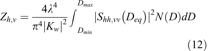
where N(D) is the DSD, D_eq is the raindrop equivolumetric diameter in mm, D_min and D_max stand for the minimum and maximum drop diameter of the DSDs, S_hh,vv (D) are the backscattering co-polar components of the complex scattering matrix S of a drop, f_hh,vv (D) are the forward scattering amplitudes at horizontal and vertical polarization states, and ℜ is the real part of the complex number. The equivolumetric diameter D_eq is related to the axis ratio of a raindrop and discussed in the next section.

3 Raindrop shape models

The principle of polarimetric radar measurement is based on drops being oblate in shape, not spherical (as is the case for single polarization radar). Generally, drop sizes smaller than 1 mm are spherical, but the shape becomes more oblate as the size increases. The drop shapes are exemplified by the ratio between the maximum vertical and horizontal axis, the axis ratio (b/a), as a function of its equivolumetric diameter (D_eq ). The representation of axis ratio with respect to the equivolumetric diameter plays a central role in the definition of polarimetric radar signatures. Furthermore, the information of axis ratio is important for radar rainfall algorithms development and for derivation of the DSDs using polarimetric radar signatures Z_H , Z_DR and K_DP (Beard et al., 2010; Hagen and Meischner, 2000; Thurai and Bringi, 2005). Additionally, to simulate the polarimetric radar signatures from DSD measurements, one must assume a relationship between b/a and D_eq (Pepler et al., 2011; Thurai et al., 2007). The derivation of the DSDs, the estimation of rainfall rates or the simulation can all be hampered to a significant extent due to a small error in the axis ratio (Bringi and Chandrasekar, 2001).

Figure 1.

Illustration of different raindrop shape models (D_eq vs b/a).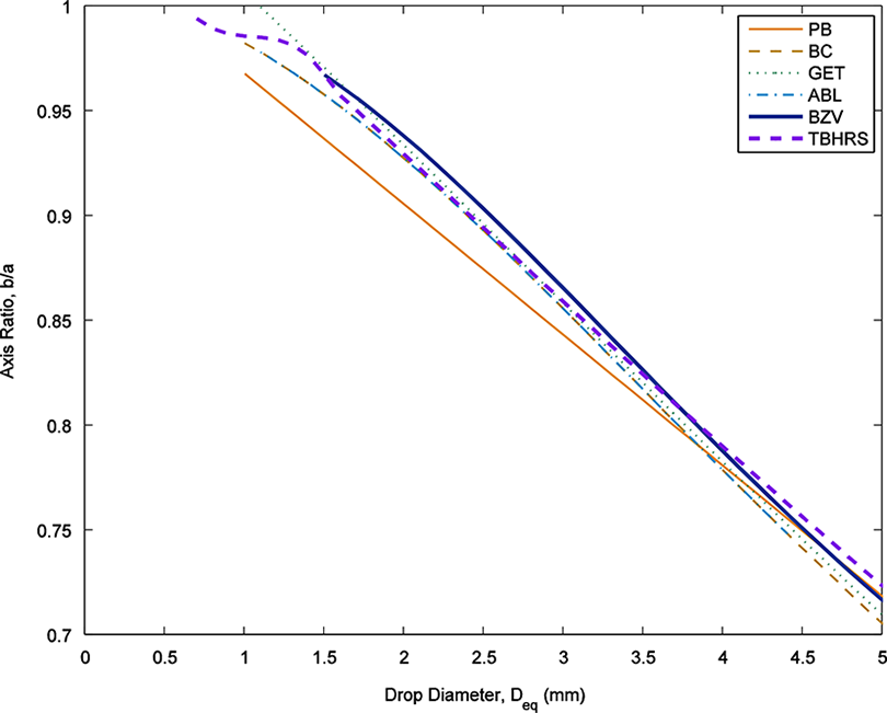

A number of raindrop shape models have been proposed by several researchers from laboratory, field and modelling investigations (see Beard et al., 2010, for an inclusive review). The first realistic raindrop shape was measured by Pruppacher and Beard (1970) (hereinafter named PB). The PB model is conceptualized in the laboratory using a vertical low turbulence wind tunnel to suspend water droplets. The drop shape was revealed in this experiment by taking a photograph, and a linear equilibrium relationship was found with equivalent spherical diameters, as:

\begin{aligned} P B \begin{matrix} \frac{b}{a} = 1.03 - 0.062 (D_{e q}) \\ (1 \leq D_{e q} \leq 9 m m) \end{matrix} \end{aligned}

The PB model was extensively used to construct the theory of polarimetry and for development of rain estimators (Gorgucci et al., 2009). However, it was later found that raindrops are less oblate than foreseen in PB. Five different raindrop shape models are commonly quoted in polarimetric radar studies: the Beard and Chuang (1987) model (hereinafter named BC), Goddard et al. (1994) model (GET), Andsager et al. (1999) model (ABL), Brandes et al. (2002) model (BZV) and Thurai et al. (2007) model (TBHRS), given in equations 16 –20, respectively (see Figure 1):

\begin{aligned} B C \begin{matrix} \frac{b}{a} = 1.0048 + 5.7 \times 10^{- 4} (D_{e q}) \\ - 2.628 \times 10^{- 2} (D_{e q}^{2}) \\ + 3.682 \times 10^{- 3} (D_{e q}^{3}) \\ - 1.677 \times 10^{- 4} (D_{e q}^{4}) \end{matrix} \end{aligned}

(1 \leq D_{e q} \leq 7 m m)

\begin{aligned} G E T \begin{matrix} \frac{b}{a} = 1.075 + 6.5 \times 10^{- 2} (D_{e q}) \\ - 3.6 \times 10^{- 3} (D_{e q}^{2}) \\ + 4.0 \times 10^{- 4} (D_{e q}^{3}) \end{matrix} \end{aligned}

(1.1 \leq D_{e q} \leq 5 m m)

\begin{aligned} A B L \begin{matrix} \frac{b}{a} = 1.012 - 0.01445 (D_{e q}) \\ - 1.028 \times 10^{- 2} (D_{e q}^{2}) \end{matrix} \end{aligned}

(1.1 \leq D_{e q} \leq 4 . 4 m m)

\begin{aligned} B Z V \begin{matrix} \frac{b}{a} = 0.9951 + 2.51 \times 10^{- 2} (D_{e q}) \\ - 3.644 \times 10^{- 2} (D_{e q}^{2}) \\ + 5.303 \times 10^{- 3} (D_{e q}^{3}) \\ - 2.492 \times 10^{- 4} (D_{e q}^{4}) \end{matrix} \end{aligned}

(D_{e q} > 1 . 5 m m)

\begin{aligned} T B H R S \begin{matrix} \frac{b}{a} = 1.065 - 6.25 \times 10^{- 2} (D_{e q}) \\ - 3.99 \times 10^{- 3} (D_{e q}^{2}) \\ + 7.66 \times 10^{- 4} (D_{e q}^{3}) \\ - 4.095 \times 10^{- 5} (D_{e q}^{4}) \end{matrix} \end{aligned}

(D_{e q} > 1 . 5 m m)

\begin{aligned} \frac{b}{a} = 1.173 - 0.5165 (D_{e q}) + 0.4698 (D_{e q}^{2}) \\ - 0.1317 (D_{e q}^{3}) - 8.5 \times 10^{- 3} (D_{e q}^{4}) \end{aligned}

(0. 7 < D_{e q} < 1 . 5 m m)

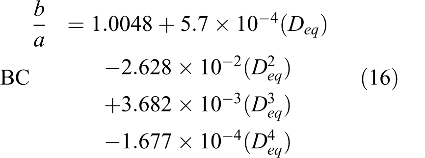
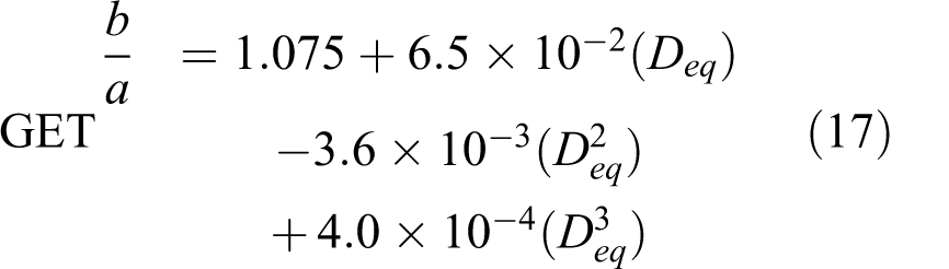
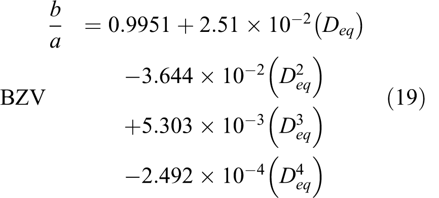
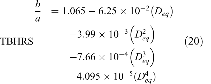
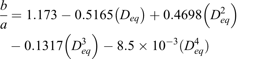
The BC model is based on the numerical methods through observation of water droplets’ aerodynamic pressure at terminal velocity which introduces the equilibrium condition between surface tension and hydrostatic pressure. Although the model is found to be in good agreement with the follow-on studies conducted by Bringi et al. (1998) and Chandrasekar et al. (1988) using aircraft probes, the oscillation phenomenon has not been accounted for in the model. When the larger diameter drops fall at higher terminal velocity than the smaller drops, collisions occur, resulting in oscillations. Raindrop oscillations and their causes were assessed by Brandes et al. (2002), Thurai and Bringi (2005), Tokay and Beard (1996) and others in field experiments. They concluded that the oscillating drops are more spherical than the small drops; this is a perturbation factor in polarimetric radar rainfall estimation. This oscillation characteristic has been addressed in the other models.

Briefly summarizing, the GET model is a composite model of two proposals given by Beard and Chuang (1987) and Goddard and Cherry (1984). The ABL model is from laboratory and field investigations for oscillations of moderate to large raindrops by a seven-storey fall column; it considers raindrops with higher average axis ratio as transverse mode oscillations. The BZV model is derived from experimental data that combines observations from past studies of Andsager et al. (1999), Beard and Kubesh (1991), Chandrasekar et al. (1988) and Pruppacher and Pitter (1971), and considers drop shapes that are significantly more spherical than that of equilibrium, in particular for diameters of 1–4 mm. The TBHRS model is from the recent 80 m fall bridge experiment, where artificial drops are generated from a pipe on an 80 m bridge, allowing drop oscillations to fall under calm conditions. The drops are then captured using a 2D video disdrometer, and the derived axis ratios agree with those of BZV. The model suggests using Beard and Kubesh (1991) fit for 0.7< D_eq < 1.5 mm.

The aforementioned models appear in many polarimetric radar studies (e.g. Gorgucci et al., 2000; Ryzhkov et al., 2005b; Teschl et al., 2008), but no definitive conclusion is evident for which model should be used for radar applications (Gorgucci and Baldini, 2009). As noted above, the effect of different raindrop shape size relation on the polarimetric radar signatures, in particular with the three intrinsic parameters Z_H , Z_DR and K_DP , has been investigated (Gorgucci et al., 2006; Keenan et al., 2001), and the rainfall estimators, R(K_DP ) and R(Z_DR , K_DP ) are affected by underlying raindrop shape models, while R(Z_H , Z_DR ) is less sensitive (Lee, 2007; Matrosov, 2010; Teschl et al., 2008). The same applies for the DSD retrievals, which implies that the retrieval results are subject to the raindrop shape assumptions.

Another factor that needs to be considered in polarimetric radar measurements is the canting angle distribution of a raindrop (Bringi et al., 2008). As an example, an examination of canting angle distribution from the polarimetric radar measurements is presented in Ryzhkov et al. (2002). On average, the canting angle as Gaussian distribution with a zero mean and standard deviation in the range of 5–12° is generally mentioned in the literature (Bringi et al., 2008; Huang et al., 2008).

4 Drop size distributions

In radar meteorology, the DSD assumption as an exponential distribution has a long history (e.g. Marshall and Palmer, 1948). The exponential distribution is defined using two parameters, and given as:

N (D) = N_{0} exp (- \land D)

where N(D) is the number of raindrops per unit volume per unit size, D is the drop diameter in mm, N₀ is the number concentration parameter in mm^-1-µ m^-3, and Λ is the slope parameter in mm^-1.

Two parameters are not enough to describe the volumetric distribution of raindrops; so, to better describe the natural variation of DSDs, Ulbrich and Atlas (1998) proposed the gamma distribution, with µ being the distribution shape parameter:

N (D) = N_{0} D^{μ} exp (- \land D)

Note that, when µ = 0, gamma DSD becomes the same as the exponential DSD. Nevertheless, in this gamma model, N₀ is dependent on µ and has no physical basis when µ ≠ 0 (Vulpiani et al., 2006). In order to address this issue, the normalization notion has been introduced by Willis (1984), and acknowledged by several authors in different studies (Bringi et al., 2003; Illingworth and Blackman, 2002; Lee et al., 2004; Testud et al., 2001). According to Bringi et al. (2003) and Testud et al. (2001), the normalized gamma DSD model is given as:

N (D) = N_{w} f (μ) {(\frac{D}{D_{0}})}^{μ} e x p [- (3.67 + μ) \frac{D}{D_{0}}]

with:

N_{w} = \frac{{3.67}^{4}}{π ρ_{w}} (\frac{10^{3} W}{D_{0}^{4}})

f (μ) = \frac{6 (3.67 + μ)^{μ + 4}}{{3.67}^{4} Γ (μ + 4)}

where N(D) is the number of raindrops per unit volume per unit size, D₀ is the median volume drop diameter in mm, N_w is the normalized drop concentration in mm^-1 mm^-3, µ is the shape parameter (unitless), W is the liquid water content in g m^-3, and ρ_w is the density of water in g cm^-3. Meanwhile, the mass weighted mean drop diameter (D_m ) can be related to the median volume diameter (D₀ ) as:

\frac{D_{0}}{D_{m}} = \frac{3.67 + μ}{4 + μ}

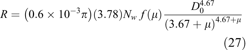
Finally, assuming the raindrop versus terminal velocity relationship ( $v = 3.78 D^{0.67}$ ) given by Atlas and Ulbrich (1977), the rain rate can be expressed as (Bringi and Chandrasekar, 2001):

R = (0.6 \times 10^{- 3} π) (3.78) N_{w} f (μ) \frac{D_{0}^{4.67}}{(3.67 + μ)^{4.67 + μ}}

A device called a disdrometer is usually employed to measure the DSDs. Several types of disdrometers, having merits and demerits for DSD measurements, exist; for their description, associated measurement errors and data processing, see Cao and Zhang (2009), Leinonen et al. (2012), Montopoli et al. (2008), Tapiador et al. (2010) and Tokay et al. (2002, 2005).

Figure 2.

An example of normalized gamma fitting of the measured DSDs from the Chilbolton Joss-Waldvogel disdrometer. The solid lines represent the distribution for µ.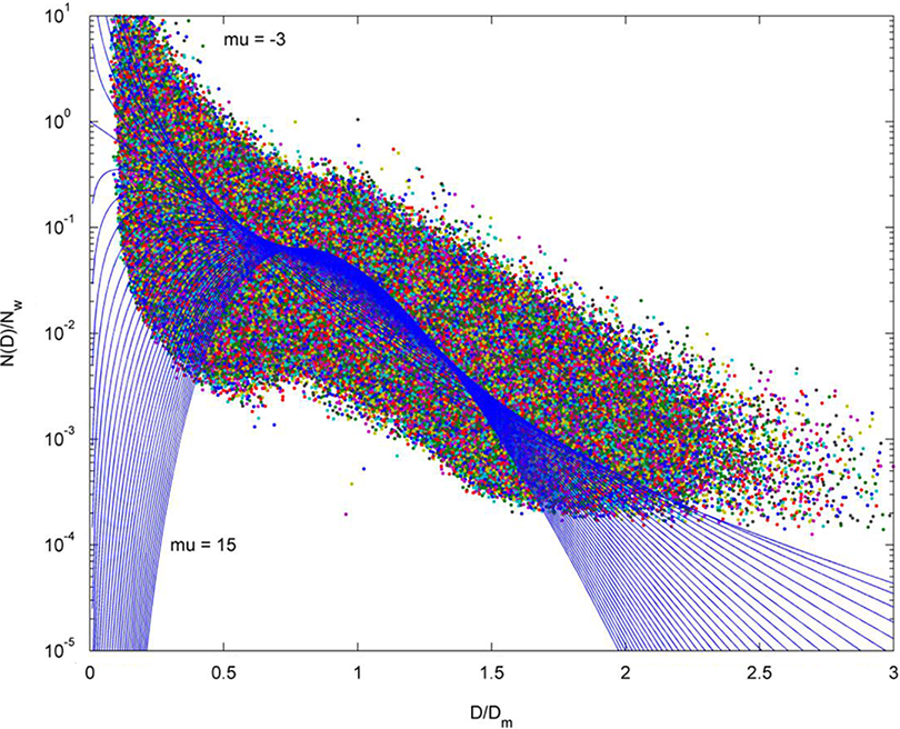

An example of normalized gamma fitting of the measured DSDs from the Chilbolton Joss-Waldvogel disdrometer data is illustrated in Figure 2. In this figure, the abscissa represents the normalized drop diameter and the ordinate represents the scaled data N(D)/N_w . One can observe that the measured DSDs are well bounded by the scaled gamma functions over a wide range of μ. High values of μ indicate a more truncated spectrum. After parameterizing the DSDs, it is straightforward to simulate the polarimetric radar signatures. For this, the T-matrix scattering simulation technique is commonly adopted as per the methodology described in Mishchenko et al. (2000) for non-spherical hydrometeors. As such, if drop size distribution is assumed as normalized gamma model, the three intrinsic polarimetric signatures Z_h , Z_DR and K_DP become (Bringi et al., 2002):

Z_{h} = N_{w} F_{1} (μ) D_{0}^{7}

Z_{D R} = F_{2} (μ, D_{0})

K_{D P} = N_{w} F_{3} (μ, D_{0})

where F represents a functional form.

Note that the normalized gamma DSD model has an advantage over the non-normalized gamma DSD model in that the three normalized gamma DSD parameters are independent in nature and liquid water content does not change corresponding to µ (Illingworth and Blackman, 2002). The normalization method makes it possible to clearly differentiate the rain types into stratiform and convective regimes (Islam et al., 2012d, 2012f). Moreover, the normalization method is very useful in accord with the polarimetric radar measurements. Intuitively, the Z_DR is proportional to the D₀ , while K_DP is related to the product N_w and D₀ . For this reason, it has become common to represent the DSDs as the normalized gamma distribution for various algorithms and model developments, such as for rainfall algorithms developments, attenuation correction methods, and DSD retrievals (Anagnostou et al., 2008a; Bringi et al., 2011b; Thurai et al., 2008; Vulpiani et al., 2009).

III Polarimetric radar signatures and their potentials

1 Reflectivity (Z_H , Z_V)

Reflectivity factors at horizontal and vertical polarization are proportional to the sum of the contributions from the backscattering cross-sections of all hydrometeors (equation 5). They provide a straightforward idea of the intensity of a precipitation episode: the more reflectivity, the more intense the precipitation episode would be. However, for the same precipitation particle size, Z_H and Z_V values from ice particles will be lower than that of the liquid particles. The dielectric constant of ice particles is relatively low compared to the liquid particles. In rain, Z_H values are larger than Z_V . Unquestionably, the Z_H is the most commonly used parameter so far. From the early era of radar meteorology, the Z-R relationship has been extensively used for rain rate estimation. Nevertheless, a long-standing argument continues regarding the reliability of the Z-R relation and its associated uncertainties. Mainly, the uncertainties are allied with DSD variations in space and time (Abdella and Alfredsen, 2010; Islam et al., 2012b, 2012f; Kozu et al., 2006; Martner et al., 2008; Prat and Barros, 2009; Steiner et al., 2004) and with instrumental errors in the measurement of DSD (Campos and Zawadzki, 2000; Salles and Creutin, 2003). With the advent of polarimetry, incorporating Z_H with some other polarimetric signatures, e.g. Z_DR and K_DP , more accurate rain rate estimation is possible in principle, compared to the conventional Z-R relation (Gourley et al., 2010; Maki et al., 2005).

In addition to the use of Z_H for rain rate estimates, it has been recognized that the Z_H information can infer the presence of clutter echoes (Chang et al., 2009; Delrieu et al., 2009; Hubbert et al., 2009a, 2009b; Silberstein et al., 2008). Further, the vertical profile of reflectivity can confirm the existence of a bright band or melting layer in the atmosphere (Fabry and Zawadzki, 1995; Rico-Ramirez and Cluckie, 2007; Rico-Ramirez et al., 2005, 2007; Zhang and Qi, 2010; Zhang et al., 2008). In general terms, the bright band is associated with melting of hydrometeors, thus reflecting enhanced radar signal Z_H . A bright band in a stratiform event recorded by the Chilbolton advanced meteorological radar (CAMRA) is shown in Figure 3. The enhanced characteristic of Z_H signal is evident herein at around 2.8 km height, indicating the existence of the melting layer. The corresponding polarimetric signatures confirm this statement. However, other studies have also reported that higher Z_H values are associated with hail events (Heinselman and Ryzhkov, 2006; Lopez and Sanchez, 2009).

Figure 3.

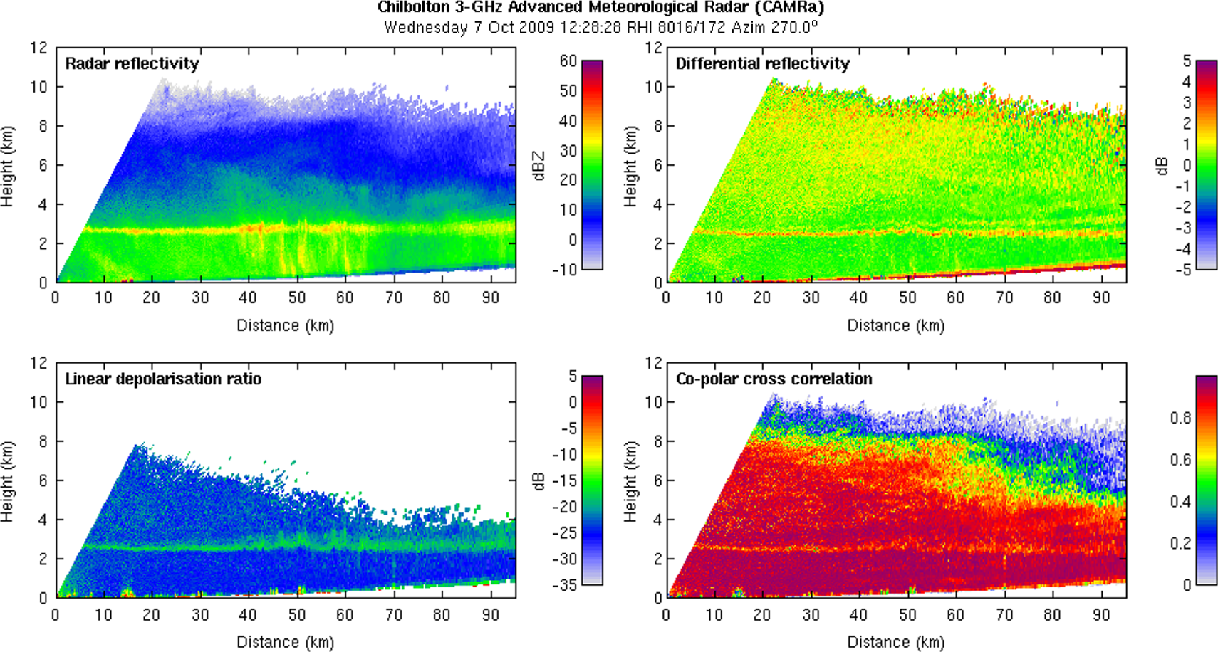
A typical example of the Chilbolton 3 GHz advanced meteorological radar range height indicator (RHI) scan depicting the polarimetric radar signatures Z_H , Z_DR , LDR and ρ_HV in a stratiform event. The presence of bright band signature is evident at around 2.8 km height.

Z_H and Z_V are, however, sensitive to the system gain bias or radar calibration error (Gourley et al., 2009; Park and Lee, 2010). At higher frequencies (shorter wavelengths), Z_H and Z_V are also affected by attenuation as the radar beam passes through high intense precipitation media, and thus could cause underestimation of radar rainfall estimation (Katsumata et al., 2008; Kramer and Verworn, 2009; Kramer et al., 2005; Rahimi et al., 2006; Rico-Ramirez, 2012). Thus the reflectivity factors need to be corrected for attenuation before possible use.

2 Differential reflectivity (Z_DR)

The Z_DR is the ratio of reflectivity at horizontal and vertical polarization (equation 6). It is directly related to the axis ratio, shape and size of particles. More specifically, it is the quantity of the reflectivity-weighted mean axis ratio of the DSDs. In Rayleigh approximation, if the produced axis ratio is less than 1 the Z_DR values will be positive, while for an axis ratio greater than 1 negative Z_DR values will be produced. Usually, small raindrops are spherical in shape. Thus, the measured Z_DR values in small raindrops will be near to zero. But, as the drop diameter increases, the raindrop shape becomes more oblate. That means large values of Z_DR are produced for large rain particles. Nevertheless, as hail tumbles while falling, it produces a Z_DR of 0 dB. On the other hand, compared with rain particles, ice particles have a lower dielectric constant. So, even though ice particles are oblate in shape, they will have low values of Z_DR . The values tend to increase when oblate ice particles become wet. Likewise, the melting layer contains a large amount of melted wet particles. That is why high Z_DR values are observed in the melting layer (e.g. see Figure 3), and therefore Z_DR is identified as a good indicator of melting layer (Brandes and Ikeda, 2004; Ikeda et al., 2005; Shusse et al., 2011). Furthermore, due to the fact that Z_DR has diverse characteristics in different hydrometeor types, it has widely been accepted as a useful polarimetric signature for hydrometeor classification (Dolan and Rutledge, 2009; Evaristo et al., 2010; Park et al., 2009) (bearing in mind that the Z_DR signature may differ from one band to another in the presence of hail due to resonance scattering; Kaltenboeck and Ryzhkov, 2013).

Additionally, because of its direct relationship to the mean particle shape and size, Z_DR can be used to retrieve the microphysical DSD parameters, N_w , D₀ and μ. A straightforward power law relationship exists between D₀ and Z_DR (D₀ = aZ_DR ^b ) (Bringi et al., 2002; Williams and May, 2008), by which D₀ can be retrieved (also true for D_m ; see Elmzoughi et al., 2011; Matrosov, 2011). Once D₀ is retrieved, N_w and μ can also be obtained by means of Z_H , Z_DR and/or K_DP (Anagnostou et al., 2008a, 2008b; Islam et al., 2012a).

Given the capability of Z_DR for providing raindrop information, it can further be used in combination with Z_H and/or K_DP for improved rainfall rate algorithms. The algorithm R(Z_H , Z_DR ) has been used to improve the accuracy of rain rate estimates compared to the conventional Z-R relation (Tabary et al., 2011). More specifically, this algorithm has been exploited as suitable in low rainfall rate regimes. For high rainfall rate regimes, the formulation of R(Z_DR , K_DP ) has also been investigated by several authors (Cifelli et al., 2011; Jorgensen et al., 2011; Ryzhkov et al., 2005b, 2005c). However, Z_DR should be calibrated within 0.1–0.2 dB accuracy (Ryzhkov et al., 2005a); if Z_DR is not accurately calibrated, the rainfall estimates may be degraded significantly. Such degradation can be worse than the conventional Z-R relation. Moreover, as stated earlier, Z_DR is near to 0 dB in hail, thus the R(Z_H , Z_DR ) algorithm will deliver high rainfall rates if rain is mixed with hail. So Z_DR should be avoided for rainfall rate estimation with hail present (Ryzhkov et al., 2005b).

Furthermore, the Z_DR ‘arc’ is considered as indicative of a kinematic property of supercell storms (Kumjian and Ryzhkov, 2008; Snyder et al., 2013). The indication is based on a vertical shear, which is quite difficult to observe using conventional Doppler radar. The indicator explains the low-level storm-relative environmental helicity (SREH), a measure of the streamwise component of environmental vorticity. The Z_DR ‘column’ has also been reported with its coincidence to thunderstorm updrafts (Loney et al., 2002; Snyder et al., 2013). Another capability of Z_DR is that it can provide significant information of clutter echoes through the use of its texture (Friedrich et al., 2009; Rico-Ramirez et al., 2009).

Although Z_DR is independent of radar concentration, because Z_DR is a product of Z_H and Z_V , the bias in Z_DR may be introduced due to the mismatch between the horizontal (H) and vertical (V) channels (Liu et al., 2010). Thus Z_DR requires additional care of offset correction and calibration. Intrinsically, 0 dB of Z_DR for Bragg scatterers in a clear atmosphere represent the precision of the calibration (Melnikov et al., 2011a). Moreover, it can also be affected due to propagation and attenuation at high frequencies; therefore, the Z_DR also requires the attenuation correction pre-processing step prior to use.

3 Differential propagation phase (Φ_DP) and specific differential propagation phase (K_DP)

The Φ_DP is a measure of the difference of phases between horizontally and vertically polarized electromagnetic waves (equation 10). In comparison with vertically polarized returns, horizontally polarized electromagnetic waves experience larger phase shifts when propagating through horizontally oriented precipitation media, such as raindrops. So horizontally polarized waves propagate at lower velocity than vertically polarized waves and lag behind. As such, Φ_DP can provide information about the shape of the particles. As the radar beam propagates, horizontally oriented particles will provide increasing positive Φ_DP with range and vertically oriented particles will provide decreasing negative Φ_DP with range. For spherical particles or those particles having no preferred orientation, such as snow and ice crystals, Φ_DP is typically zero. Φ_DP is also not affected by hail that appears spherical on radar due to tumbling (Φ_DP ∼ 0). In rain, the Φ_DP magnitude increases with respect to the oblateness of drop sizes. However, unlike Z_DR , Φ_DP values are dependent on concentration in a radar pulse volume. The greater the concentration, the higher the Φ_DP values will be. At the same time, in the bright band or melting layer, Φ_DP articulates high values, demonstrating the presence of snowflakes. In addition, the Φ_DP fluctuates to a larger extent and becomes very noisy in the case of non-meteorological echoes (Islam et al., 2012c). Hence, Φ_DP is a very useful parameter for clutter identification. It has been shown that the Φ_DP texture is the outperformed signature among all polarimetric signatures (with exception of LDR) for clutter identification (Islam et al., 2012c). However, the Φ_DP is a cumulative measure and cannot provide the information within particular ranges. Thus retrieving precipitation characteristics information on a gate by gate basis with Φ_DP is not possible. K_DP , however, can be used to acquire quantitative precipitation information on a particular region and normally K_DP is computed over several range bins (e.g. 5 km or more). Wang and Chandrasekar (2009) and Hu et al. (2012) exemplified estimating K_DP as range derivative of Φ_DP .

The advantage of K_DP (or Φ_DP ) is that it is independent of radar calibrations. Therefore, absolute calibration of the co-polar reflectivity is possible using differential phase shift in rain (Thurai and Hanado, 2005). Possibly the highest potential of Φ_DP , however, could be its immunity to attenuation, and thus its use for correcting radar reflectivity and differential reflectivity for attenuation. A trend of larger phase shifts usually exists along the beam as portions of the electromagnetic spectrum are being lost due to scattering and absorption in the precipitation media, which leads to weakening of the radar signals. Figure 4 provides such an example of decreasing Z_H along the radial due to attenuation effects, in which the corresponding Φ_DP profile confirms the attenuation experience by showing large phase shifts.

Figure 4.

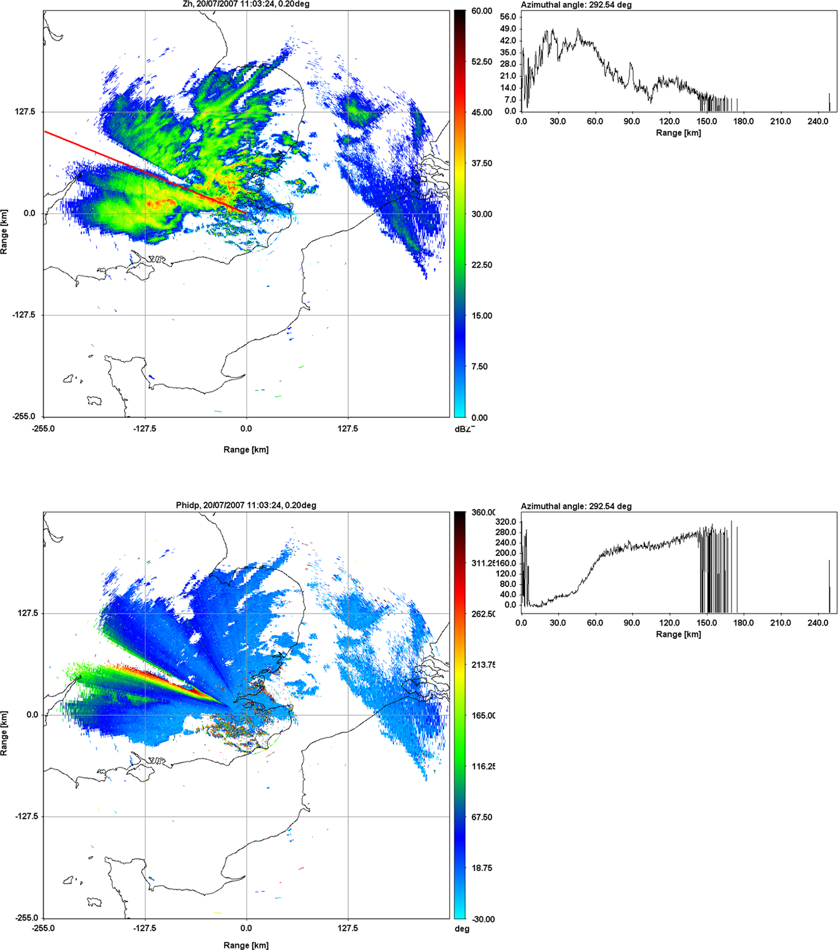
The Thurnham C-band polarimetric radar plan position indicator (PPI) of Z_H and Φ_DP signatures in an extreme attenuation event. Corresponding Z_H and Φ_DP profiles for a particular attenuated beam are also displayed in the right panel.

A linear relationship of specific attenuation A_H and specific differential attenuation A_DP against K_DP exists, following Gu et al. (2011):

A_{H} = α K_{D P}^{b}

A_{D P} = β K_{D P}^{c}

Here the coefficients are dependent upon several factors, such as radar wavelength, raindrop temperature, drop shapes, and DSDs. Generally speaking, the attenuation experience for a given rain rate is relatively small and negligible at S-band compared to higher frequencies such as C-band and X-band. Therefore, attenuation needs to be corrected for at those frequencies. A number of attenuation correction algorithms exploiting Φ_DP (related to K_DP ) have been proposed (Bringi et al., 2001; Smyth and Illingworth, 1998; Vulpiani et al., 2008). Subsequently, the Φ_DP based correction procedures have been successfully applied in order to correct the radar reflectivity and differential reflectivity at different frequencies (Anagnostou et al., 2009; Gourley et al., 2007; Hu et al., 2010; Snyder et al., 2010; Tabary et al., 2009; Xue et al., 2009). Again, since, K_DP is immune to radar attenuation, the R(K_DP ) estimator has been an encouraging choice for radar rainfall estimates at attenuating frequencies such as the X-band (Anagnostou et al., 2010; Borowska et al., 2011; Gosset et al., 2010; Wang and Chandrasekar, 2010). The use of the R(K_DP ) estimator at C-band (Silvestro et al., 2009; Vulpiani et al., 2012) and S-band has also been reported. Particularly in hail or with rain/hail mixture, R(K_DP ) estimator has proved as useful (Giangrande and Ryzhkov, 2008).

Furthermore, the derivation of K_DP from Φ_DP is already cumbersome. K_DP is noisy along the beam path, and in light rain intensities the noise is greater and K_DP becomes less effective (below 0.2 or 0.3 deg km^-1). Accordingly, based on the noise of Φ_DP , a filtering treatment is required to smooth the signal (Hu et al., 2012; Hubbert and Bringi, 1995).

4 Linear depolarization ratio (LDR)

The LDR is the logarithm of the ratio of the cross-polar power to the co-polar power received (equation 7). A horizontally polarized radar signal is transmitted, but both horizontally and vertically polarized signals are measured when they return; thus it measures the depolarization of the horizontally polarized signal scattered into the vertical direction. Several procedures are available to estimate the depolarization from linear H and V polarization measurements (e.g. Chandrasekar and Bharadwaj, 2009; Hubbert et al., 2003; Matrosov, 2004). Indeed, this depolarization can find the characteristics of associated hydrometeors, such as shape, uniformity, dielectric constant, thermodynamic phase and degree of canting. Note that, for a perfect spherical particle, no depolarization will occur to the horizontally transmitted signal, thus theoretically resulting in LDR to infinity. If the target particle is not a perfect sphere, cross-polar power return will be produced. For spherical particles, such as rain and snow, cross-polar measurements are very low compared to the co-polar measurements. Therefore, typical LDR values lie from –35 dB to –15 dB in rain and snow. Further limiting of LDR values to –40 dB may provide more insights into the precipitation characteristics at subfreezing temperature (Bringi et al., 2011a). Also, the melting layer exhibits a distinct peak of the LDR values of –15 dB, on average (Kowalewski and Peters, 2010). Additionally, several studies have investigated the characteristics of LDR for various types of hydrometeors, such as hail, graupel, snow crystals, and mixed phase hydrometeors (Depue et al., 2007; Hopper et al., 1991; Islam et al., 2013; Kennedy et al., 2001; Lim et al., 2005; Sato and Okamoto, 2006).

Alternatively, higher values of LDR are often associated with the clutter echoes, and it has been successively used in suppressing the ground clutter and anomalous propagation. In a simple way, clutter signals can easily be rejected by using a high threshold of LDR. However, the simple threshold based technique has the limitation of clutter rejection, because LDR increases with decreasing signal to noise ratio (SNR). Nevertheless, the use of LDR within a spectral polarimetry perception is established for improved clutter suppression (Unal, 2009).

Lastly, LDR is free from radar calibration errors and independent of concentration; nevertheless, it is prone to high noise and propagation effects. Moreover, no quantitative information of rain rates can be achieved using this signature.

5 Correlation coefficient (ρ_HV)

The correlation coefficient (ρ_HV ) is the correlation of the time series of continual observations of reflectivity at horizontal and vertical polarization (equation 8). The theoretical ρ_HV values range between 0 and 1. Commonly, ρ_HV is a good measure of the uniformity of the hydrometeor orientations and shapes. If the shape of the hydrometeor is uniform and regular, the ρ_HV will be near to unity; for non-uniform and irregular targets, the ρ_HV will be considerably lower. The value of ρ_HV decreases as the diversity of the hydrometeor shape increases (Zrnic et al., 1993). As a result, ρ_HV can identify non-meteorological echoes as well as various types of meteorological echoes. For non-meteorological echoes such as clutter and biological targets, the two polarizations (H and V) have different amplitudes. Therefore the correlation ρ_HV becomes low. Again, since raindrops and snow are nearly spherical in shape, the H polarization is almost as same as the vertical polarization. That implies the ρ_HV in rain and snow is almost unity (∼0.98). In the case of mixed hydrometeors present in a radar volume, ρ_HV is lower. Besides, hail particles have a lower value of ρ_HV , and with increasing hail sizes ρ_HV value decreases. Therefore ρ_HV has been extensively used for hydrometeor classification (e.g. Keenan, 2003; Liu and Chandrasekar, 2000; Marzano et al., 2010). Due to its straightforward hydrometeor classification quantifying rain, melting particles and snow, it is a valuable polarimetric signature for melting layer detection (Boodoo et al., 2010; Brandes and Ikeda, 2004; Giangrande et al., 2008; Matrosov et al., 2007).

However, ρ_HV can degrade meaningfully and become smeared with range due to decreasing SNR and beam broadening effects. For instance, in the RHI scan provided in Figure 3 the beam broadens with increasing distance. This effect implies that at greater range the radar beam is too wide, and sometimes may be wider than the melting layer. In consequence, detection of melting layer at longer distance may not be accurate.

IV Opportunities and challenges

The quantitative precipitation estimation (QPE) should be regarded as one of the most important topics in polarimetric radar remote sensing of precipitation (e.g. Kabeche et al., 2012; Kato et al., 2012; Ventura et al., 2012). For meteorology, the polarimetric QPE should be able to contribute towards improved and accurate weather monitoring and prediction of atmospheric hazards (rainfall extremes). Li and Mecikalski (2010) reported a data assimilation scheme that utilizes the polarimetric signatures to assimilate into a regional mesoscale model with the three-dimensional variational data assimilation (3DVAR) system. They demonstrated the benefit of utilizing polarimetric radar signatures in the assimilation scheme and how it improved in short-term storm forecasting for a mesoscale convective system. Nevertheless, the authors clarified that in their study only the warm rain microphysical processes were considered, but not the ice microphysics. Thus, the results provided an initial understanding of the benefits of the radar polarimetry, and there is still room for improvements in forecasting the precipitation system.

For hydrology, the polarimetric QPE will be able to provide an improved estimation of precipitation propagating to hydrological models, thus leading to better hydrological forecasts, because precipitation is their main driving force (Berne and Krajewski, 2013; Gourley et al., 2010; Rico-Ramirez et al., 2012). Additionally, polarimetric QPE is focused on rain estimates, and estimating snowfall is considered as a challenging task. Although Schneebeli et al. (2013) identified snow through radar polarimetry, the quantification of snowfall is not well developed. Moreover, in mountainous regions, complex orographic issues degrade polarimetric radar data quality, and hinder precipitation retrieval (Vulpiani et al., 2012).

Polarimetric radar is creating significant opportunities for precipitation science, in both research and operational fields. In consequence, meteorological agencies across the world are turning to polarimetric radar technology, and these will provide even more opportunities for basic and applied research in the upcoming years.

Footnotes

Funding

This research received no specific grant from any funding agency in the public, commercial, or not-for-profit sectors.

References

Abdella

Alfredsen

(2010) Long-term evaluation of gauge-adjusted precipitation estimates from a radar in Norway. Hydrology Research 41: 171–192.

Akita

Yoshida

Nakamura

. (2011) Effects of charge distribution in thunderstorms on lightning propagation paths in Darwin, Australia. Journal of the Atmospheric Sciences 68: 719–726.

Anagnostou

Vivekanandan

. (2008a) Comparison of two raindrop size distribution retrieval algorithms for X-band dual polarization observations. Journal of Hydrometeorology 9: 589–600.

Anagnostou

Vulpiani

. (2008b) Evaluation of X-band polarimetric-radar estimates of drop-size distributions from coincident S-band polarimetric estimates and measured raindrop spectra. IEEE Transactions on Geoscience and Remote Sensing 46: 3067–3075.

Anagnostou

Kalogiros

Anagnostou

. (2009) Experimental results on rainfall estimation in complex terrain with a mobile X-band polarimetric weather radar. Atmospheric Research 94: 579–595.

Anagnostou

Kalogiros

Anagnostou

. (2010) Performance evaluation of high-resolution rainfall estimation by X-band dual-polarization radar for flash flood applications in mountainous basins. Journal of Hydrology 394: 4–16.

Andsager

Beard

Laird

(1999) Laboratory measurements of axis ratios for large raindrops. Journal of the Atmospheric Sciences 56: 2673–2683.

Atlas

Ulbrich

(1977) Path-integrated and area-integrated rainfall measurement by microwave attenuation in 1–3 cm band. Journal of Applied Meteorology 16: 1322–1331.

Battan

(1973) Radar Observation of the Atmosphere. Chicago, IL: University of Chicago Press.

10.

Battan

Braham

(1956) A study of convective precipitation based on cloud and radar observations. Journal of Meteorology 13: 587–591.

11.

Beard

Chuang

(1987) A new model for the equilibrium shape of raindrops. Journal of the Atmospheric Sciences 44: 1509–1524.

12.

Beard

Kubesh

(1991) Laboratory measurements of small raindrop distortion. Part 2: Oscillation frequencies and modes. Journal of the Atmospheric Sciences 48: 2245–2264.

13.

Beard

Bringi

Thurai

(2010) A new understanding of raindrop shape. Atmospheric Research 97: 396–415.

14.

Bent

(1946) Radar detection of precipitation. Journal of Meteorology 3: 78–84.

15.

Berne

Krajewski

(2013) Radar for hydrology: Unfulfilled promise or unrecognized potential? Advances in Water Resources 51: 357–366.

16.

Bolen

Chandrasekar

(2003) Quantitative estimation of Tropical Rainfall Mapping Mission precipitation radar signals from ground-based polarimetric radar observations. Radio Science 38: 8056.

17.

Boodoo

Hudak

Donaldson

. (2010) Application of dual-polarization radar melting-layer detection algorithm. Journal of Applied Meteorology and Climatology 49: 1779–1793.

18.

Borowska

Zrnic

Ryzhkov

. (2011) Polarimetric estimates of a 1-month accumulation of light rain with a 3-cm wavelength radar. Journal of Hydrometeorology 12: 1024–1039.

19.

Brandes

Ikeda

(2004) Freezing-level estimation with polarimetric radar. Journal of Applied Meteorology 43: 1541–1553.

20.

Brandes

Zhang

Vivekanandan

(2002) Experiments in rainfall estimation with a polarimetric radar in a subtropical environment. Journal of Applied Meteorology 41: 674–685.

21.

Bringi

Chandrasekar

(2001) Polarimetric Doppler Weather Radar: Principles and Applications. Cambridge: Cambridge University Press.

22.

Bringi

Chandrasekar

Hubbert

. (2003) Raindrop size distribution in different climatic regimes from disdrometer and dual-polarised radar analysis. Journal of the Atmospheric Sciences 60: 354–365.

23.

Bringi

Chandrasekar

Xiao

(1998) Raindrop axis ratios and size distributions in Florida rainshafts: An assessment of multiparameter radar algorithms. IEEE Transactions on Geoscience and Remote Sensing 36: 703–715.

24.

Bringi

Hoferer

Brunkow

. (2011a) Design and performance characteristics of the new 8.5-m dual-offset Gregorian antenna for the CSU-CHILL radar. Journal of Atmospheric and Oceanic Technology 28: 907–920.

25.

Bringi

Huang

Chandrasekar

. (2002) A methodology for estimating the parameters of a gamma raindrop size distribution model from polarimetric radar data: Application to a squall-line event from the TRMM/Brazil campaign. Journal of Atmospheric and Oceanic Technology 19: 633–645.

26.

Bringi

Keenan

Chandrasekar

(2001) Correcting C-band radar reflectivity and differential reflectivity data for rain attenuation: A self-consistent method with constraints. IEEE Transactions on Geoscience and Remote Sensing 39: 1906–1915.

27.

Bringi

Rico-Ramirez

Thurai

(2011b) Rainfall estimation with an operational polarimetric C-band radar in the United Kingdom: Comparison with a gauge network and error analysis. Journal of Hydrometeorology 12: 935–954.

28.

Bringi

Thurai

Brunkow

(2008) Measurements and inferences of raindrop canting angles. Electronics Letters 44: 1425–1426.

29.

Bringi

Williams

Thurai

. (2009) Using dual-polarised radar and dual-frequency profiler for DSD characterization: A case study from Darwin, Australia. Journal of Atmospheric and Oceanic Technology 26: 2107–2122.

30.

Campos

Zawadzki

(2000) Instrumental uncertainties in Z-R relations. Journal of Applied Meteorology 39: 1088–1102.

31.

Cao

Zhang

(2009) Errors in estimating raindrop size distribution parameters employing disdrometer and simulated raindrop spectra. Journal of Applied Meteorology and Climatology 48: 406–425.

32.

Cao

Yeary

Zhang

(2012) Efficient ways to learn weather radar polarimetry. IEEE Transactions on Education 55: 58–68.

33.

Celano

Porcu

Alberoni

. (2008) On the combined use of satellite multispectral and radar polarimetric measurements to infer cloud microphysics. Meteorology and Atmospheric Physics 101: 111–126.

34.

Chandrasekar

Bharadwaj

(2009) Orthogonal channel coding for simultaneous co- and cross-polarization measurements. Journal of Atmospheric and Oceanic Technology 26: 45–56.

35.

Chandrasekar

Bolen

Gorgucci

(2003) Microphysical cross validation of spaceborne radar and ground polarimetric radar. IEEE Transactions on Geoscience and Remote Sensing 41: 2153–2165.

36.

Chandrasekar

Cooper

Bringi

(1988) Axis ratios and oscillations of raindrops. Journal of the Atmospheric Sciences 45: 1323–1333.

37.

Chandrasekar

Hou

Smith

. (2008) Potential role of dual-polarization radar in the validation of satellite precipitation measurements: Rationale and opportunities. Bulletin of the American Meteorological Society 89: 1127–1145.

38.

Chandrasekar

Zafar

(2005) Estimation of raindrop size distribution from spaceborne radar observations. IEEE Transactions on Geoscience and Remote Sensing 43: 1078–1086.

39.

Chang

Lin

Jou

BJD

. (2009) An application of reflectivity climatology in constructing radar hybrid scans over complex terrain. Journal of Atmospheric and Oceanic Technology 26: 1315–1327.

40.

Chong

Georgis

Bousquet

. (2000) Real-time wind synthesis from Doppler radar observations during the mesoscale alpine programme. Bulletin of the American Meteorological Society 81: 2953–2962.

41.

Cifelli

Chandrasekar

Lim

. (2011) A new dual-polarization radar rainfall algorithm: Application in Colorado precipitation events. Journal of Atmospheric and Oceanic Technology 28: 352–364.

42.

Cluckie

Rico-Ramirez

(2004) Weather radar technology and future developments. In: Chen

Takara

Cluckie

. (eds) GIS and Remote Sensing in Hydrology, Water Resources and Environment. Wallingford: International Association of Hydrological Sciences, 11–20.

43.

Collier

(2002) Developments in radar and remote-sensing methods for measuring and forecasting rainfall. Philosophical Transactions of the Royal Society of London Series A – Mathematical Physical and Engineering Sciences 360: 1345–1361.

44.

Collier

Larke

May

(1983) A weather radar correction procedure for real-time estimation of surface rainfall. Quarterly Journal of the Royal Meteorological Society 109: 589–608.

45.

Delrieu

Boudevillain

Nicol

. (2009) Bollene-2002 Experiment: Radar quantitative precipitation estimation in the Cevennes-Vivarais region, France. Journal of Applied Meteorology and Climatology 48: 1422–1447.

46.

Depue

Kennedy

Rutledge

(2007) Performance of the hail differential reflectivity (HDR) polarimetric radar hail indicator. Journal of Applied Meteorology and Climatology 46: 1290–1301.

47.

Dolan

Rutledge

(2009) A theory-based hydrometeor identification algorithm for X-band polarimetric radars. Journal of Atmospheric and Oceanic Technology 26: 2071–2088.

48.

Doviak

Zrnic

(1993) Doppler Radar and Weather Observations. New York: Academic Press.

49.

Doviak

Bringi

Ryzhkov

. (2000) Considerations for polarimetric upgrades to operational WSR-88D radars. Journal of Atmospheric and Oceanic Technology 17: 257–278.

50.

Eito

Aonashi

(2009) Verification of hydrometeor properties simulated by a cloud-resolving model using a passive microwave satellite and ground-based radar observations for a rainfall system associated with the Baiu Front. Journal of the Meteorological Society of Japan 87: 425–446.

51.

Elmzoughi

Abdelfattah

Del Rio

. (2011) Optimal rain rate estimation algorithm for light and heavy rain using polarimetric measurements. Natural Hazards and Earth System Sciences 11: 3067–3079.

52.

Evaristo

Scialom

Viltard

. (2010) Polarimetric signatures and hydrometeor classification of West African squall lines. Quarterly Journal of the Royal Meteorological Society 136: 272–288.

53.

Fabry

Zawadzki

(1995) Long-term radar observations of the melting layer of precipitation and their interpretation. Journal of the Atmospheric Sciences 52: 838–851.

54.

Friedrich

Germann

Tabary

(2009) Influence of ground clutter contamination on polarimetric radar parameters. Journal of Atmospheric and Oceanic Technology 26: 251–269.

55.

Friedrich

Hagen

Einfalt

(2006) A quality control concept for radar reflectivity, polarimetric parameters, and Doppler velocity. Journal of Atmospheric and Oceanic Technology 23: 865–887.

56.

Fritz

Chandrasekar

(2012) Simulating radar observations of precipitation at higher frequencies from lower-frequency polarimetric measurements. Journal of Atmospheric and Oceanic Technology 29: 1435–1454.

57.

Giangrande

Ryzhkov

(2008) Estimation of rainfall based on the results of polarimetric echo classification. Journal of Applied Meteorology and Climatology 47: 2445–2462.

58.

Giangrande

Krause

Ryzhkov

(2008) Automatic designation of the melting layer with a polarimetric prototype of the WSR-88D radar. Journal of Applied Meteorology and Climatology 47: 1354–1364.

59.

Goddard

JWF

Cherry

(1984) The ability of dual-polarization radar (copolar linear) to predict rainfall rate and microwave attenuation. Radio Science 19: 201–208.

60.

Goddard

JWF

Eastment

Tan

(1994) Self-consistent measurements of differential phase and differential reflectivity in rain. In: Geoscience and Remote Sensing Symposium, 1994. IGARSS ’94. Surface and Atmospheric Remote Sensing: Technologies, Data Analysis and Interpretation, International, 369–371.

61.

Gorgucci

Baldini

(2009) An examination of the validity of the mean raindrop-shape model for dual-polarization radar rainfall retrievals. IEEE Transactions on Geoscience and Remote Sensing 47: 2752–2761.

62.

Gorgucci

Baldini

Chandrasekar

(2006) What is the shape of a raindrop? An answer from radar measurements. Journal of the Atmospheric Sciences 63: 3033–3044.

63.

Gorgucci

Chandrasekar

Baldini

(2009) Can a unique model describe the raindrop shape-size relation? A clue from polarimetric radar measurements. Journal of Atmospheric and Oceanic Technology 26: 1829–1842.

64.

Gorgucci

Scarchilli

Chandrasekar

. (2000) Measurement of mean raindrop shape from polarimetric radar observations. Journal of the Atmospheric Sciences 57: 3406–3413.

65.

Gosset

Zahiri

Moumouni

(2010) Rain drop size distribution variability and impact on X-band polarimetric radar retrieval: Results from the AMMA campaign in Benin. Quarterly Journal of the Royal Meteorological Society 136: 243–256.

66.

Gourley

Giangrande

Hong

. (2010) Impacts of polarimetric radar observations on hydrologic simulation. Journal of Hydrometeorology 11: 781–796.

67.

Gourley

Illingworth

Tabary

(2009) Absolute calibration of radar reflectivity using redundancy of the polarization observations and implied constraints on drop shapes. Journal of Atmospheric and Oceanic Technology 26: 689–703.

68.

Gourley

Tabary

du Chatelet

(2007) Empirical estimation of attenuation from differential propagation phase measurements at C band. Journal of Applied Meteorology and Climatology 46: 306–317.

69.

Ryzhkov

Zhang

. (2011) Polarimetric attenuation correction in heavy rain at C band. Journal of Applied Meteorology and Climatology 50: 39–58.

70.

Hagen

Meischner

(2000) Estimation of rainfall parameters from polarimetric radar measurements with POLDIRAD. Physics and Chemistry of the Earth Part B – Hydrology Oceans and Atmosphere 25: 849–853.

71.

Heinselman

Ryzhkov

(2006) Validation of polarimetric hail detection. Weather and Forecasting 21: 839–850.

72.

Herzegh

Jameson

(1992) Observing precipitation through dual-polarization radar measurements. Bulletin of the American Meteorological Society 73: 1365–1374.

73.

Holleman

Huuskonen

Gill

. (2010) Operational monitoring of radar differential reflectivity using the sun. Journal of Atmospheric and Oceanic Technology 27: 881–887.

74.

Holt

(2001) An analysis of depolarization of circular polarization in S-band radar sensing of Alberta storms. Journal of Atmospheric and Oceanic Technology 18: 1567–1576.

75.

Hooper

JEN

Kippax

(1950) Radar echoes from meteorological precipitation. Proceedings of the Institution of Electrical Engineers – London 97: 89–97.

76.

Hopper

Illingworth

Caylor

. (1991) Bright-band errors in rainfall measurement: Identification and correction using linearly polarised radar returns. In: Cluckie

Collier

(eds) Hydrological Applications of Weather Radar. Chichester: Ellis Horwood, 240–249.

77.

Liu

Chu

. (2010) Study of different attenuation correction methods in association with rainfall estimation for X-band polarimetric radars. Acta Meteorologica Sinica 24: 602–613.

78.

Liu

Wang

(2012) A quality assurance procedure and evaluation of rainfall estimates for C-band polarimetric radar. Advances in Atmospheric Sciences 29: 144–156.

79.

Huang

Bringi

Thurai

(2008) Orientation angle distributions of drops after an 80-m fall using a 2D video disdrometer. Journal of Atmospheric and Oceanic Technology 25: 1717–1723.

80.

Hubbert

Bringi

(1995) An iterative filtering technique for the analysis of copolar differential phase and dual-frequency radar measurements. Journal of Atmospheric and Oceanic Technology 12: 643–648.

81.

Hubbert

Bringi

Brunkow

(2003) Studies of the polarimetric covariance matrix. Part I: Calibration methodology. Journal of Atmospheric and Oceanic Technology 20: 696–706.

82.

Hubbert

Dixon

Ellis

(2009a) Weather radar ground clutter. Part II: Real-time identification and filtering. Journal of Atmospheric and Oceanic Technology 26: 1181–1197.

83.

Hubbert

Dixon

Ellis

. (2009b) Weather radar ground clutter. Part I: Identification, modeling, and simulation. Journal of Atmospheric and Oceanic Technology 26: 1165–1180.

84.

Hunter

(1954) Polarization of radar echoes from meteorological precipitation. Nature 173: 165–166.

85.

Ikeda

Brandes

Rasmussen

(2005) Polarimetric radar observation of multiple freezing levels. Journal of the Atmospheric Sciences 62: 3624–3636.

86.

Illingworth

Blackman

(2002) The need to represent raindrop size spectra as normalized gamma distributions for the interpretation of polarization radar observations. Journal of Applied Meteorology 41: 286–297.

87.

Islam

Rico-Ramirez

Han

(2012a) Tree-based genetic programming approach to infer microphysical parameters of the DSDs from the polarization diversity measurements. Computers and Geosciences 48: 20–30.

88.

Islam

Rico-Ramirez

Han

(2012b) Variability of rain microphysics using long-term disdrometer observations. In: Moore

Cole

Illingworth

(eds) Weather Radar and Hydrology. Wallingford: International Association of Hydrological Sciences, 147–152.

89.

Islam

Rico-Ramirez

Han

. (2012c) Artificial intelligence techniques for clutter identification with polarimetric radar signatures. Atmospheric Research 109–110: 95–113.

90.

Islam

Rico-Ramirez

Han

. (2012d) Using S-band dual polarised radar for convective/stratiform rain indexing and the correspondence with AMSR-E GSFC profiling algorithm. Advances in Space Research 50: 1383–1390.

91.

Islam

Rico-Ramirez

Han

. (2012e) Performance evaluation of the TRMM precipitation estimation using ground-based radars from the GPM validation network. Journal of Atmospheric and Solar-Terrestrial Physics 77: 194–208.

92.

Islam

Rico-Ramirez

Han

. (2013) Fuzzy logic based melting layer recognition from 3 GHz dual polarization radar: Appraisal with NWP model and radio sounding observations. Theoretical and Applied Climatology 112: 317–338.

93.

Islam

Rico-Ramirez

Thurai

. (2012f) Characteristics of raindrop spectra as normalized gamma distribution from a Joss–Waldvogel disdrometer. Atmospheric Research 108: 57–73.

94.

Jorgensen

Hanshaw

Schmidt

. (2011) Value of a dual-polarised gap-filling radar in support of southern California post-fire debris-flow warnings. Journal of Hydrometeorology 12: 1581–1595.

95.

Kabeche

Ventura

JFI

Fradon

. (2012) X-band polarimetric quantitative precipitation estimation: The RHYTMME project. In: Moore

Cole

Illingworth

(eds) Weather Radar and Hydrology. Wallingford: International Association of Hydrological Sciences, 176–181.

96.

Kaltenboeck

Ryzhkov

(2013) Comparison of polarimetric signatures of hail at S and C bands for different hail sizes. Atmospheric Research 123: 323–336.

97.

Kato

Maki

(2009) Localized heavy rainfall near Zoshigaya, Tokyo, Japan on 5 August 2008 observed by X-band polarimetric radar – preliminary analysis. SOLA 5: 89–92.

98.

Kato

Maki

Iwanami

. (2012) Quantitative precipitation estimate by complementary application of X-band polarimetric radar and C-band conventional radar. In: Moore

Cole

Illingworth

(eds) Weather Radar and Hydrology. Wallingford: International Association of Hydrological Sciences, 169–175.

99.

Katsumata

Ushiyama

Yoneyama

. (2008) Combined use of TRMM/PR and disdrometer data to correct reflectivity of ground-based radars. SOLA 4: 101–104.

100.

Keenan

(2003) Hydrometeor classification with a C-band polarimetric radar. Australian Meteorological Magazine 52: 23–31.

101.

Keenan

Carey

Zrnic

. (2001) Sensitivity of 5-cm wavelength polarimetric radar variables to raindrop axial ratio and drop size distribution. Journal of Applied Meteorology 40: 526–545.

102.

Kennedy

Rutledge

Petersen

. (2001) Polarimetric radar observations of hail formation. Journal of Applied Meteorology 40: 1347–1366.

103.

Kim

Maki

Lee

(2010) Retrieval of three-dimensional raindrop size distribution using X-band polarimetric radar data. Journal of Atmospheric and Oceanic Technology 27: 1265–1285.

104.

Kowalewski

Peters

(2010) Analysis of Z-R relations based on LDR signatures within the melting layer. Journal of Atmospheric and Oceanic Technology 27: 1555–1561.

105.

Kozu

Reddy

Mori

. (2006) Seasonal and diurnal variations of raindrop size distribution in Asian monsoon region. Journal of the Meteorological Society of Japan 84A: 195–209.

106.

Kramer

Verworn

(2009) Improved radar data processing algorithms for quantitative rainfall estimation in real time. Water Science and Technology 60: 175–184.

107.

Kramer

Verworn

Redder

(2005) Improvement of X-band radar rainfall estimates using a microwave link. Atmospheric Research 77: 278–299.

108.

Kumjian

Ryzhkov

(2008) Polarimetric signatures in supercell thunderstorms. Journal of Applied Meteorology and Climatology 47: 1940–1961.

109.

Lee

(2007) Sources of errors in precipitation measurements by polarimetric radar: Sensitivity of polarimetric parameters to drop deformation. Journal of the Korean Meteorological Society 43: 41–57.

110.

Lee

Zawadzki

Szyrmer

. (2004) A general approach to double-moment normalization of drop size distributions. Journal of Applied Meteorology 43: 264–281.

111.

Leijnse

Uijlenhoet

van de Beek

(2010) Precipitation measurement at CESAR, the Netherlands. Journal of Hydrometeorology 11: 1322–1329.

112.

Leinonen

Moisseev

Leskinen

. (2012) A climatology of disdrometer measurements of rainfall in Finland over five years with implications for global radar observations. Journal of Applied Meteorology and Climatology 51: 392–404.

113.

Leskinen

Markkula

Koistinen

. (2011) Pest insect immigration warning by an atmospheric dispersion model, weather radars and traps. Journal of Applied Entomology 135: 55–67.

114.

Mecikalski

(2010) Assimilation of the dual-polarization Doppler radar data for a convective storm with a warm-rain radar forward operator. Journal of Geophysical Research – Atmospheres 115: D16208.

115.

Lim

Chandrasekar

Bringi

(2005) Hydrometeor classification system using dual-polarization radar measurements: Model improvements and in situ verification. IEEE Transactions on Geoscience and Remote Sensing 43: 792–801.

116.

Liu

Chandrasekar

(2000) Classification of hydrometeors based on polarimetric radar measurements: Development of fuzzy logic and neuro-fuzzy systems, and in situ verification. Journal of Atmospheric and Oceanic Technology 17: 140–164.

117.

Liu

Fang

. (2010) Calibration and data quality analysis with mobile C-band polarimetric radar. Acta Meteorologica Sinica 24: 501–509.

118.

Loney

Zrnic

Straka

. (2002) Enhanced polarimetric radar signatures above the melting level in a supercell storm. Journal of Applied Meteorology 41: 1179–1194.

119.

Lopez

Sanchez

(2009) Discriminant methods for radar detection of hail. Atmospheric Research 93: 358–368.

120.

McCormick

(1979) Relationship of differential reflectivity to correlation in dual-polarization radar. Electronics Letters 15: 265–266.

121.

Maki

Park

Bringi

(2005) Effect of natural variations in rain drop size distributions on rain rate estimators of 3 cm wavelength polarimetric radar. Journal of the Meteorological Society of Japan 83: 871–893.

122.

Markkula

Leskinen

Pylkko

. (2008) Early warning system for insect migration using weather radars. Zemdirbyste-Agriculture 95: 110–115.

123.

Marks

Wolff

Carey

. (2011) Quality control and calibration of the dual-polarization radar at Kwajalein, RMI. Journal of Atmospheric and Oceanic Technology 28: 181–196.

124.

Marshall

Palmer

(1948) The distribution of raindrops with size. Journal of Meteorology 5: 165–166.

125.

Martner

Yuter

White

. (2008) Raindrop size distributions and rain characteristics in California coastal rainfall for periods with and without a radar bright band. Journal of Hydrometeorology 9: 408–425.

126.

Marzano

Botta

Montopoli

(2010) Iterative Bayesian retrieval of hydrometeor content from X-band polarimetric weather radar. IEEE Transactions on Geoscience and Remote Sensing 48: 3059–3074.

127.

Matrosov

(2004) Depolarization estimates from linear H and V measurements with weather radars operating in simultaneous transmission-simultaneous receiving mode. Journal of Atmospheric and Oceanic Technology 21: 574–583.

128.

Matrosov

(2010) Evaluating polarimetric X-band radar rainfall estimators during HMT. Journal of Atmospheric and Oceanic Technology 27: 122–134.

129.

Matrosov

(2011) Polarimetric radar-based estimates of spatial variability in characteristic sizes of raindrops in stratiform rainfall. Journal of Applied Meteorology and Climatology 50: 2514–2525.

130.

Matrosov

Clark

Kingsmill

(2007) A polarimetric radar approach to identify rain, melting-layer, and snow regions for applying corrections to vertical profiles of reflectivity. Journal of Applied Meteorology and Climatology 46: 154–166.

131.

May

Allen

Vaughan

. (2009) Aerosol and thermodynamic effects on tropical cloud systems during TWPICE and ACTIVE. Atmospheric Chemistry and Physics 9: 15–24.

132.

May

Kepert

Keenan

(2008a) Polarimetric radar observations of the persistently asymmetric structure of Tropical Cyclone Ingrid. Monthly Weather Review 136: 616–630.

133.

May

Mather

Vaughan

. (2008b) The tropical warm pool international cloud experiment. Bulletin of the American Meteorological Society 89: 629–645.

134.

Meischner

Hagen

(2000) Weather radars in Europe: Potential for advanced applications. Physics and Chemistry of the Earth Part B – Hydrology Oceans and Atmosphere 25: 813–816.

135.

Melnikov

Doviak

Zrnic

. (2011a) Mapping Bragg scatter with a polarimetric WSR-88D. Journal of Atmospheric and Oceanic Technology 28: 1273–1285.

136.

Melnikov

Zrnic

Doviak

. (2011b) Prospects of the WSR-88D radar for cloud studies. Journal of Applied Meteorology and Climatology 50: 859–872.

137.

Michaelides

Levizzani

Anagnostou

. (2009) Precipitation: Measurement, remote sensing, climatology and modeling. Atmospheric Research 94: 512–533.

138.

Mishchenko

Hovenier

Travis

(2000) Light Scattering by Nonspherical Particles: Theory, Measurements, and Applications. San Diego, CA: Academic Press.

139.

Montopoli

Marzano

Vulpiani

(2008) Analysis and synthesis of raindrop size distribution time series from disdrometer data. IEEE Transactions on Geoscience and Remote Sensing 46: 466–478.

140.

Oue

Uyeda

Shusse

(2010) Two types of precipitation particle distribution in convective cells accompanying a Baiu frontal rainband around Okinawa Island, Japan. Journal of Geophysical Research – Atmospheres 115: D02201.

141.

Park

Ryzhkov

Zrnic

. (2009) The hydrometeor classification algorithm for the polarimetric WSR-88D: Description and application to an MCS. Weather and Forecasting 24: 730–748.

142.

Park

Lee

(2010) Calibration of radar reflectivity measurements from the KMA operational radar network. Asia-Pacific Journal of Atmospheric Sciences 46: 243–259.

143.

Pepler

May

Thurai

(2011) A robust error-based rain estimation method for polarimetric radar. Part I: Development of a method. Journal of Applied Meteorology and Climatology 50: 2092–2103.

144.

Prat

Barros

(2009) Exploring the transient behavior of Z-R relationships: Implications for radar rainfall estimation. Journal of Applied Meteorology and Climatology 48: 2127–2143.

145.

Probert-Jones

(1962) The radar equation in meteorology. Quarterly Journal of the Royal Meteorological Society 88: 485–495.

146.

Pruppacher

Beard

(1970) A wind tunnel investigation of the internal circulation and shape of water drops falling at terminal velocity in air. Quarterly Journal of the Royal Meteorological Society 96: 247–256.

147.

Pruppacher

Pitter

(1971) A semi-empirical determination of the shape of cloud and rain drops. Journal of the Atmospheric Sciences 28: 86–94.

148.

Pucillo

Giaiotti

Stel

(2009) Ground wind convergence as source of deep convection initiation. Atmospheric Research 93: 437–445.

149.

Rahimi

Holt

Upton

GJG

. (2006) Attenuation calibration of an X-band weather radar using a microwave link. Journal of Atmospheric and Oceanic Technology 23: 395–405.

150.

Rico-Ramirez

(2012) Adaptive attenuation correction techniques for C-band polarimetric weather radars. IEEE Transactions on Geoscience and Remote Sensing 50: 5061–5071.

151.

Rico-Ramirez

Cluckie

(2007) Bright-band detection from radar vertical reflectivity profiles. International Journal of Remote Sensing 28: 4013–4025.

152.

Rico-Ramirez

Cluckie

(2008) Classification of ground clutter and anomalous propagation using dual-polarization weather radar. IEEE Transactions on Geoscience and Remote Sensing 46: 1892–1904.

153.

Rico-Ramirez

Bringi

Thurai

(2012) River flow simulations with polarimetric weather radar. In: Moore

Cole

Illingworth

(eds) Weather Radar and Hydrology. Wallingford: International Association of Hydrological Sciences, 466–471.

154.

Rico-Ramirez

Cluckie

Han

(2005) Correction of the bright band using dual-polarisation radar. Atmospheric Science Letters 6: 40–46.

155.

Rico-Ramirez

Cluckie

Shepherd

. (2007) A high-resolution radar experiment on the island of Jersey. Meteorological Applications 14: 117–129.

156.

Rico-Ramirez

Gonzalez-Ramirez

Cluckie

. (2009) Real-time monitoring of weather radar antenna pointing using digital terrain elevation and a Bayes clutter classifier. Meteorological Applications 16: 227–236.

157.

Roca

Berges

Brogniez

. (2010) On the water and energy cycles in the tropics. Comptes Rendus Geoscience 342: 390–402.

158.

Ryzhkov

Giangrande

Melnikov

. (2005a) Calibration issues of dual-polarization radar measurements. Journal of Atmospheric and Oceanic Technology 22: 1138–1155.

159.

Ryzhkov

Giangrande

Schuur

(2005b) Rainfall estimation with a polarimetric prototype of WSR-88D. Journal of Applied Meteorology 44: 502–515.

160.

Ryzhkov

Schuur

Burgess

. (2005c) The joint polarization experiment – polarimetric rainfall measurements and hydrometeor classification. Bulletin of the American Meteorological Society 86: 809–824.

161.

Ryzhkov

Zrnic

Hubbert

. (2002) Polarimetric radar observations and interpretation of co-cross-polar correlation coefficients. Journal of Atmospheric and Oceanic Technology 19: 340–354.

162.

Sachidananda

Zrnic

(1985) ZDR measurement considerations for a fast scan capability radar. Radio Science 20: 907–922.

163.

Salles

Creutin

(2003) Instrumental uncertainties in Z-R relationships and raindrop fall velocities. Journal of Applied Meteorology 42: 279–290.

164.

Saltikoff

Nevvonen

(2011) First experiences of the operational use of a dual-polarisation weather radar in Finland. Meteorologische Zeitschrift 20: 323–333.

165.

Sato

Okamoto

(2006) Characterization of Z(e) and LDR of nonspherical and inhomogeneous ice particles for 95-GHz cloud radar: Its implication to microphysical retrievals. Journal of Geophysical Research – Atmospheres 111: D22213.

166.

Schneebeli

Dawes

Lehning

. (2013) High-resolution vertical profiles of X-band polarimetric radar observables during snowfall in the Swiss Alps. Journal of Applied Meteorology and Climatology 52: 378–394.

167.

Schwaller

Morris

(2011) A ground validation network for the Global Precipitation Measurement mission. Journal of Atmospheric and Oceanic Technology 28: 301–319.

168.

Scialom

Faroux

Giraud

. (2009) RONSARD Radar: Implementation of dual polarization on a C-band Doppler weather radar. IEEE Geoscience and Remote Sensing Letters 6: 132–136.

169.

Scott

Krehbiel

Rison

(2001) The use of simultaneous horizontal and vertical transmissions for dual-polarization radar meteorological observations. Journal of Atmospheric and Oceanic Technology 18: 629–648.

170.

Seliga

Bringi

(1976) Potential use of radar differential reflectivity measurements at orthogonal polarizations for measuring precipitation. Journal of Applied Meteorology 15: 69–76.

171.

Seliga

Bringi

(1978) Differential reflectivity and differential phase-shift – applications in radar meteorology. Radio Science 13: 271–275.

172.

Shusse

Takahashi

Nakagawa

. (2011) Polarimetric radar observation of the melting layer in a convective rainfall system during the rainy season over the East China Sea. Journal of Applied Meteorology and Climatology 50: 354–367.

173.

Silberstein

Wolff

Marks

(2008) Ground clutter as a monitor of radar stability at Kwajalein, RMI. Journal of Atmospheric and Oceanic Technology 25: 2037–2045.

174.

Silvestro

Rebora

Ferraris

(2009) An algorithm for real-time rainfall rate estimation by using polarimetric radar: RIME. Journal of Hydrometeorology 10: 227–240.

175.

Smyth

Illingworth

(1998) Correction for attenuation of radar reflectivity using polarization data. Quarterly Journal of the Royal Meteorological Society 124: 2393–2415.

176.

Snyder

Bluestein

Venkatesh

. (2013) Observations of polarimetric signatures in supercells by an X-band mobile Doppler radar. Monthly Weather Review 141: 3–29.

177.

Snyder

Bluestein

Zhang

. (2010) Attenuation correction and hydrometeor classification of high-resolution, X-band, dual-polarised mobile radar measurements in severe convective storms. Journal of Atmospheric and Oceanic Technology 27: 1979–2001.

178.

Steiner

Smith

Uijlenhoet

(2004) A microphysical interpretation of radar reflectivity-rain rate relationships. Journal of the Atmospheric Sciences 61: 1114–1131.

179.

Tabary

Boumahmoud

Andrieu

. (2011) Evaluation of two ‘integrated’ polarimetric Quantitative Precipitation Estimation (QPE) algorithms at C-band. Journal of Hydrology 405: 248–260.

180.

Tabary

Scialom

Germann

(2001) Real-time retrieval of the wind from aliased velocities measured by Doppler radars. Journal of Atmospheric and Oceanic Technology 18: 875–882.

181.

Tabary

Vulpiani

Gourley

. (2009) Unusually high differential attenuation at C Band: Results from a two-year analysis of the French Trappes polarimetric radar data. Journal of Applied Meteorology and Climatology 48: 2037–2053.

182.

Tapiador

Checa

de Castro

(2010) An experiment to measure the spatial variability of rain drop size distribution using sixteen laser disdrometers. Geophysical Research Letters 37: L16803.

183.

Teschl

Randeu

Schönhuber

. (2008) Simulation of polarimetric radar variables in rain at S-, C-and X-band wavelengths. Advances in Geosciences 16: 27–32.

184.

Testud

Oury

Black

. (2001) The concept of ‘normalized’ distribution to describe raindrop spectra: A tool for cloud physics and cloud remote sensing. Journal of Applied Meteorology 40: 1118–1140.

185.

Thurai

Bringi

(2005) Drop axis ratios from a 2D video disdrometer. Journal of Atmospheric and Oceanic Technology 22: 966–978.

186.

Thurai

Hanado

(2005) Absolute calibration of C-band weather radars using differential propagation phase in rain. Electronics Letters 41: 1405–1406.

187.

Thurai

Huang

Bringi

(2007) Drop shapes, model comparisons, and calculations of polarimetric radar parameters in rain. Journal of Atmospheric and Oceanic Technology 24: 1019–1032.

188.

Thurai

Hudak

Bringi

(2008) On the possible use of copolar correlation coefficient for improving the drop size distribution estimates at C band. Journal of Atmospheric and Oceanic Technology 25: 1873–1880.

189.

Tokay

Beard

(1996) A field study of raindrop oscillations. Part I: Observation of size spectra and evaluation of oscillation causes. Journal of Applied Meteorology 35: 1671–1687.

190.

Tokay

Bashor

Wolff

(2005) Error characteristics of rainfall measurements by collocated Joss-Waldvogel disdrometers. Journal of Atmospheric and Oceanic Technology 22: 513–527.

191.

Tokay

Kruger

Krajewski

. (2002) Measurements of drop size distribution in the southwestern Amazon basin. Journal of Geophysical Research – Atmospheres 107(D20): 8052.

192.

Torlaschi

Holt

(1993) Separation of propagation and backscattering effects in rain for circular-polarization diversity S-band radars. Journal of Atmospheric and Oceanic Technology 10: 465–477.

193.

Torlaschi

Holt

(1998) A comparison of different polarization schemes for the radar sensing of precipitation. Radio Science 33: 1335–1352.

194.

Turk

Park

Haddad

. (2011) Constraining CloudSat-based snowfall profiles using surface observations and C-band ground radar. Journal of Geophysical Research – Atmospheres 116: D23205.

195.

Twomey

(1953) On the measurement of precipitation intensity by radar. Journal of Meteorology 10: 66–67.

196.

Ulbrich

Atlas

(1998) Rainfall microphysics and radar properties: Analysis methods for drop size spectra. Journal of Applied Meteorology 37: 912–923.

197.

Unal

(2009) Spectral polarimetric radar clutter suppression to enhance atmospheric echoes. Journal of Atmospheric and Oceanic Technology 26: 1781–1797.

198.

Unal

CMH

Moisseev

(2004) Combined Doppler and polarimetric radar measurements: Correction for spectrum aliasing and nonsimultaneous polarimetric measurements. Journal of Atmospheric and Oceanic Technology 21: 443–456.

199.

van de Beek

Leijnse

Stricker

JNM

. (2010) Performance of high-resolution X-band radar for rainfall measurement in the Netherlands. Hydrology and Earth System Sciences 14: 205–221.

200.

Ventura

JFI

Boumahmoud

Fradon

. (2012) Long-term monitoring of French polarimetric radar data quality and evaluation of several polarimetric quantitative precipitation estimators in ideal conditions for operational implementation at C-band. Quarterly Journal of the Royal Meteorological Society 138: 2212–2228.

201.

Villarini

Krajewski

(2010) Review of the different sources of uncertainty in single polarization radar-based estimates of rainfall. Surveys in Geophysics 31: 107–129.

202.

Vulpiani

Giangrande

Marzano

(2009) Rainfall estimation from polarimetric S-band radar measurements: Validation of a neural network approach. Journal of Applied Meteorology and Climatology 48: 2022–2036.

203.

Vulpiani

Marzano

Chandrasekar

. (2006) Polarimetric weather radar retrieval of raindrop size distribution by means of a regularised artificial neural network. IEEE Transactions on Geoscience and Remote Sensing 44: 3262–3275.

204.

Vulpiani

Montopoli

Passeri

. (2012) On the use of dual-polarised C-band radar for operational rainfall retrieval in mountainous areas. Journal of Applied Meteorology and Climatology 51: 405–425.

205.

Vulpiani

Tabary

Du Chatelet

. (2008) Comparison of advanced radar polarimetric techniques for operational attenuation correction at C band. Journal of Atmospheric and Oceanic Technology 25: 1118–1135.

206.

Wang

Carey

(2005) The development and structure of an oceanic squall-line system during the South China Sea Monsoon Experiment. Monthly Weather Review 133: 1544–1561.

207.

Wang

Chandrasekar

(2009) Algorithm for estimation of the specific differential phase. Journal of Atmospheric and Oceanic Technology 26: 2565–2578.

208.

Wang

Chandrasekar

(2010) Quantitative precipitation estimation in the CASA X-band dual-polarization radar network. Journal of Atmospheric and Oceanic Technology 27: 1665–1676.

209.

Wen

Hong

Zhang

. (2011) Cross validation of spaceborne radar and ground polarimetric radar aided by polarimetric echo classification of hydrometeor types. Journal of Applied Meteorology and Climatology 50: 1389–1402.

210.

Williams

May

(2008) Uncertainties in profiler and polarimetric DSD estimates and their relation to rainfall uncertainties. Journal of Atmospheric and Oceanic Technology 25: 1881–1887.

211.

Willis

(1984) Functional fits to some observed drop size distributions and parameterization of rain. Journal of the Atmospheric Sciences 41: 1648–1661.

212.

Xue

Tong

Zhang

(2009) Simultaneous state estimation and attenuation correction for thunderstorms with radar data using an Ensemble Kalman Filter: Tests with simulated data. Quarterly Journal of the Royal Meteorological Society 135: 1409–1423.

213.

Yamamoto

Mega

Ikeno

. (2011) Doppler velocity measurement of portable X-band weather radar equipped with magnetron transmitter and IF digital receiver. IEICE Transactions on Communications E94B: 1716–1724.

214.

Zhang

(2010) A real-time algorithm for the correction of brightband effects in radar-derived QPE. Journal of Hydrometeorology 11: 1157–1171.

215.

Zhang

Langston

Howard

(2008) Brightband identification based on vertical profiles of reflectivity from the WSR-88D. Journal of Atmospheric and Oceanic Technology 25: 1859–1872.

216.

Zrnic

Ryzhkov

(1999) Polarimetry for weather surveillance radars. Bulletin of the American Meteorological Society 80: 389–406.

217.

Zrnic

Balakrishnan

Ziegler

. (1993) Polarimetric signatures in the stratiform region of a mesoscale convective system. Journal of Applied Meteorology 32: 678–693.

An overview of the remote sensing of precipitation with polarimetric radar

Abstract

Keywords

I Introduction

II Polarimetric radar rationale

1 Background

2 Backscattering and propagation

3 Raindrop shape models

4 Drop size distributions

III Polarimetric radar signatures and their potentials

1 Reflectivity (ZH , ZV)

2 Differential reflectivity (ZDR)

3 Differential propagation phase (ΦDP) and specific differential propagation phase (KDP)

4 Linear depolarization ratio (LDR)

5 Correlation coefficient (ρHV)

IV Opportunities and challenges

Footnotes

Funding

References

1 Reflectivity (Z_H , Z_V)

2 Differential reflectivity (Z_DR)

3 Differential propagation phase (Φ_DP) and specific differential propagation phase (K_DP)

5 Correlation coefficient (ρ_HV)