Review of dependence modeling in hydrology and water resources

Abstract

Various methods have been developed over the past five decades for dependence modeling of multivariate variables in hydrology and water resources, but there has been no overall review of techniques commonly used in the field. This paper, therefore, introduces several methods focusing on dependence structure modeling, including parametric distribution, entropy, copula, and nonparametric. Recent advances in modeling dependences mainly reside in nonlinear dependence modeling (including extreme dependence) with flexible marginal distributions, and in high-dimension dependence modeling via the vine copula construction with flexible dependence structures. Strengths and limitations of different methods and avenues for future research, such as dependence modeling in a changing climate, are discussed to aid water resource planners and managers in the selection and application of suitable techniques.

Keywords

Dependence modeling multivariate distribution parametric distribution entropy copula nonparametric method temporal dependence spatial dependence extreme dependence

I Introduction

In water resources planning and management, statistical inference and analysis is the common tool to estimate the risk of hydrologic events of interest (Haan, 2002; Singh, 1992; Singh et al., 2007). Numerous efforts have been devoted to this topic for hydrologic applications in the univariate case, such as frequency analysis. However, hydrologic events, such as floods and droughts, are generally associated with several properties (Favre et al., 2004; Hao and Singh, 2015a; Koutsoyiannis et al., 1998; Zhang and Singh, 2007). For example, rainfall is characterized by intensity and depth, a drought by duration and severity, and a flood by peak and duration. In these cases, analysis of risk associated with a given event using a simple univariate approach may lead to some underestimation or overestimation of the risk. Meanwhile, it is generally required to study the relationship between different variables or events, such as precipitation, temperature, soil moisture, streamflow, and storm, and the occurrence of hydrologic events at multiple locations may be of particular interest, such as precipitation at different sites. As such, dependence structures among different random variables or their properties have to be taken into account in the modeling and analysis of hydrologic events, at the core of which is the construction of multivariate distribution functions to model different dependence structures. Considering that the well-known properties of univariate distributions are extensively reported in the literature (Balakrishnan et al., 1994; Johnson et al., 2005) and that marginal properties of univariate variables may be separated in dependence modeling through appropriate methods, this study focuses on the dependence modeling of multivariate variables in hydrology and water resources.

Several types of dependences have been commonly adopted in hydrologic practices and have to be modeled with suitable tools. The traditional measure of dependence is the Pearson’s product-moment correlation coefficient, which is computed based on the assumption of normal distribution to measure the linear dependence. This is commonly adopted in statistical frameworks, such as the autoregressive moving average (ARMA) model to characterize the linear dependence among multivariate random variables in hydrology, such as precipitation or streamflow. However, since the normal assumption may not hold in many cases and the linear dependence is too restrictive to characterize far more complicated dependence structures in practice, rank correlations, such as the Spearman and Kendall correlations, have also been commonly used as alternative dependence measures to characterize the nonlinear dependence of hydrological variables, as witnessed in recent decades through models, such as copula (Genest and Favre, 2007; Nelsen, 2006). Extremes, especially joint extremes, may lead to serious damages to the society and environment and modeling dependences of extremes between rare events has attracted much attention recently (Davison and Huser, 2015; Dutfoy et al., 2014). In this case, measures, such as the Pearson correlation coefficient or Spearman rank correlation coefficient, are not appropriate, since they measure the dependence in the main body of data. The tail dependence coefficient is a suitable choice as a dependence measure when the dependence of multivariate random variables in the tail part is of particular interest, and has been commonly used in investigating hydroclimatic extremes, such as precipitation and temperature (Beersma and Buishand, 2004; Serinaldi et al., 2015; Thibaud et al., 2013; Vandenberghe et al., 2010). For example, in the context of multivariate frequency analysis, it is of critical importance to model the dependence in the extreme (or tail) region to estimate the risk adequately (Poulin et al., 2007; Salvadori and De Michele, 2007). Characterizing these types of dependences requires suitable models to fully capture the dependence structure of multivariate hydrologic variables.

The construction of a multivariate distribution in modeling different dependence structures is an active area of research (Johnson et al., 2002; Kotz et al., 2000; Sarabia Alzaga and Gómez Déniz, 2011), which encompasses various applications in hydrology and water resources, such as frequency analysis, streamflow or rainfall simulation, geo-statistical interpolation, bias correction, and downscaling. A variety of methods, such as multivariate parametric distribution (Balakrishnan and Lai, 2009; Johnson et al., 2002), entropy (Jaynes, 2003; Singh, 2013), copula (Joe, 1997; Nelsen, 2006), and nonparametric (Lall, 1995; Scott, 1992), have been developed to model various dependence structures of multivariate variables through the construction of joint or conditional distribution. For example, the development of copulas has resulted in a surge in building multivariate distributions to model the nonlinear dependence of hydroclimatic variables in a suite of applications (Genest and Favre, 2007; Hao and Singh, 2015b; Jaworski et al., 2010; Salvadori and De Michele, 2007; Schoelzel and Friederichs, 2008). These methods provide different ways of modeling dependence structures with their own advantages and disadvantages and the selection of suitable methods to model the specific dependence accurately is an important task and remaining challenge.

Although a few reviews have been reported on each method, a comprehensive overview of different methods for dependence modeling seems lacking. This study provides a review of different methods for dependence modeling in various applications in hydrology and water resources, together with strengths and limitations of different methods and avenues for future applications. Because of the vastness of each method, the review is confined to the dependence modeling of multivariate hydrological variables through the construction of multivariate distributions in the continuous context. This paper is organized as follows. After the discussion of different dependence measures in Section II, various methods, including the parametric distribution, entropy, copula, and nonparametric methods, are discussed in Sections III, IV, V, and VI, respectively. Discussions are provided in Section VII, followed by conclusions in Section VIII.

II Dependence measures

A dependence measure between variables describes how two (or more) variables cluster together. The measures and concepts of dependence in a multivariate setting include the linear correlation, rank (or monotone) association, positive quadrant dependence, tail dependence, and others (Hao and Singh, 2015b; Joe, 2014; Mari and Kotz, 2001; Nelsen, 2006). Here we focus on three types of dependence measures that are most commonly used in hydrology and water resources, the Pearson linear correlation that measures the linear dependence, rank correlation that measures the degree of monotonic dependence, and the tail dependence regarding the dependence in the extreme (tail) part.

2.1 Pearson linear correlation

For two random variables X and Y, the Pearson correlation coefficient (ρ) can be expressed as

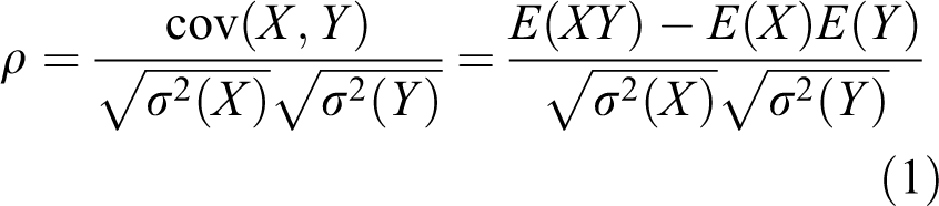
ρ = \frac{cov (X, Y)}{\sqrt{σ^{2} (X)} \sqrt{σ^{2} (Y)}} = \frac{E (X Y) - E (X) E (Y)}{\sqrt{σ^{2} (X)} \sqrt{σ^{2} (Y)}}

where cov(X, Y) is the covariance of X and Y; and σ²(X) and σ²(Y) are variances of X and Y, respectively. The range of correlation coefficient ρ is from −1 to 1 with 1 representing a perfect increasing linear relationship and –1 a perfect decreasing linear relationship.

The Pearson correlation coefficient measures linear dependence between two variables. It is among the most commonly used dependence measures in practice, since its computation is straightforward and is a natural dependence measure under multivariate normal distribution (MVN; Embrechts et al., 2002). The Pearson correlation coefficient has been commonly used to measure the dependence between hydrologic variables in a variety of applications to describe how two metrics match (e.g. simulation or forecast versus observation). The drawbacks are that it only measures the linear dependence and is not invariant under general monotonic transformations. Hydrological data are generally non-Gaussian and thus the inference procedures regarding the dependence based on linear correlation may be misleading. When the assumption of linear correlation does not hold in general or nonlinear dependences (or dependence in a particular region) are required, other dependence measures may be resorted to.

2.2 Rank correlation

The rank (or monotone) association refers to the dependence when one variable increases and the other tends to either increase or decrease. Spearman’s rho and Kendall’s tau rank correlations are the two most commonly used dependence measures in cases when the Pearson correlation coefficient is inappropriate or even misleading. Both measures range from –1 to 1 with limits –1 and 1 representing perfectly negative and perfectly positive association, respectively.

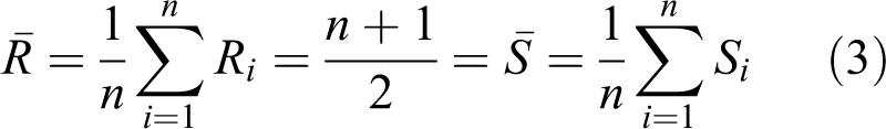
Spearman’s rho (ρ_s ) is defined in a similar way as the Pearson correlation coefficient but is based on the rank of observations instead. For the observed pairs (X_i , Y_i ), i = 1, 2,…, n, define R_i as the rank of X_i and S_i as the rank of Y_i . The Spearman’s rho is defined as (Genest and Favre, 2007)

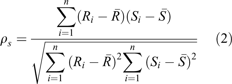
ρ_{s} = \frac{\sum_{i = 1}^{n} (R_{i} - \bar{R}) (S_{i} - \bar{S})}{\sqrt{\sum_{i = 1}^{n} {(R_{i} - \bar{R})}^{2} \sum_{i = 1}^{n} {(S_{i} - \bar{S})}^{2}}}

where

\bar{R} = \frac{1}{n} \sum_{i = 1}^{n} R_{i} = \frac{n + 1}{2} = \bar{S} = \frac{1}{n} \sum_{i = 1}^{n} S_{i}

The Kendall’s tau (ρ _τ) is another well-known measure of dependence, which is defined as (Genest and Favre, 2007)

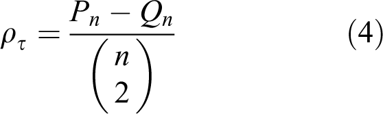
ρ_{τ} = \frac{P_{n} - Q_{n}}{(\begin{matrix} n \\ 2 \end{matrix})}

where P_n and Q_n are the concordant and discordant pairs of observations. The pairs of observations (x_i , y_i ) and (x_j , y_j ) are said to be concordant if (x_i – x_j )(y_i – y_j ) > 0, while they are said to be discordant if (x_i – x_j )(y_i – y_j ) < 0.

Both the Spearman and Kendall correlations are measures of monotone dependences. The distinct advantage of the monotone dependence over the linear correlation coefficient is that it is invariant under the monotonic transformation of variables. For example, the transformed vector (exp(X), exp(Y)) will have the same Spearman and Kendall correlations as the original vector (X, Y). The Spearman or Kendall correlations have been commonly used for measuring the nonlinear dependence among different hydrologic variables and overcome the drawbacks of the Pearson correlation coefficient to some extent. However, these correlations may fall short in measuring the dependence in the extreme or tail region.

2.3 Tail dependence

The Pearson, Kendall, and Spearman correlations give the overall level or strength of the association between random variables. However, these measures do not reveal the dependence in the specific part of the distribution (such as the tail or extreme part), which may be of greater interest in practical applications of extreme modeling. The tail dependence measures the probability of two random variables taking extremes and is a suitable measure when the dependence of extremes is of particular concern.

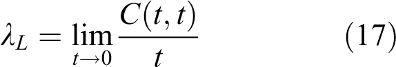
For tail dependence modeling of two random variables, the dependence in the upper right quadrant or the lower left quadrant is generally of greater interest. Let the marginal distributions of two random variables X and Y be F(x) and G(y).The upper (and lower) tail dependence parameter λ_U (and λ_L ) that a variable u (or v) exceeds a given quantile t can be defined as (Nelsen, 2006)

λ_{U} = \lim_{t \to 1} P (Y > G^{- 1} (t)) | X > F^{- 1} (t))

λ_{L} = \lim_{t \to 0} P (Y \leq G^{- 1} (t) | X \leq F^{- 1} (t))

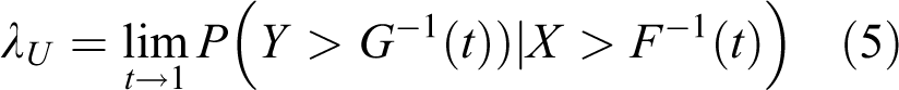
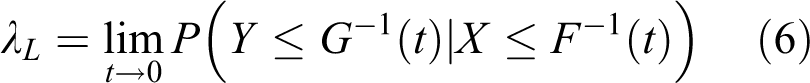
It is said that there is upper (or lower) dependence if 0 < λ_U ≤ 1 (or 0 < λ_L ≤ 1) and no upper (or lower) dependence if λ_U = 0 (or λ_L = 0).The tail dependence is related to the conditional probability of one variable exceeding a certain value when the other exceeds some value, which measures the strength of the dependence in the lower or upper tails of a multivariate distribution (Trivedi and Zimmer, 2005). It is useful in summarizing how extremes tend to occur simultaneously and has been commonly used to aid the modeling of multivariate extremes.

III Parametric distribution

The study of parametric distributions and their properties has been a persistent theme in the statistical literature. Certain parametric distributions, such as the Weibull and gamma distribution, have been commonly used in water resources planning and management (Haan, 2002). A standard approach to obtain a multivariate distribution results from the immediate extension from univariate distributions. In the multivariate setting, a variety of parametric families of multivariate distributions have been documented in earlier works (Johnson et al., 1997, 2002; Kotz et al., 2000), including, but not limited to, the multivariate Gaussian, t, gamma, extreme value, Burr, and logistic distributions. The multivariate parametric distributions have several drawbacks (Favre et al., 2004), including (1) the marginal distribution of each variable generally shares the same form; (2) the modeling of dependence is determined or affected by the parameters of marginal distributions; and (3) the extension of the distribution form to a higher dimension is limited or not clear. Moreover, the capability of these models to represent flexible dependence structures (e.g. nonlinear dependence) is generally limited. These drawbacks restrict wide applications of multivariate parametric distributions in hydrology and water resources. The entropy method (Singh, 2013), copula method (Nelsen, 2006), and nonparametric method (Lall, 1995) that will be introduced in the following sections are among the most commonly used methods to address these issues. In this section, the commonly used multivariate parametric distributions for modeling dependence in hydrology and water resources will be introduced.

3.1 Multivariate parametric distribution with fixed marginals

A variety of multivariate parametric distributions have been extended from univariate distributions for the modeling of dependence among different variables. For the bivariate case, parametric distributions, such as the bivariate normal (or log-normal), bivariate gamma, and bivariate extreme value distribution, have been applied for the modeling of hydrologic variables for different purposes (Adamson et al., 1999; Bacchi et al., 1994; Goel et al., 1998; Nadarajah, 2007; Yue, 1999; Yue et al., 2001). For these models, the marginal distributions of two variables are generally the same. Among parametric distributions, the normal distribution plays a central role in classical statistics and can be naturally extended to the multivariate Gaussian or normal distribution, which is the most well-known and useful continuous multivariate parametric distribution for the modeling of multivariate variables in many areas of applications (Tong, 1990; Wilks, 2011). The popularity of MVN partly results from the theoretical background of the Central Limit Theorem (CLT) and its easy extension to higher dimensions (Wilks, 2011). Related distributions, such as multivariate extensions of Student’s t, Fischer’s F distributions, or the multivariate Gaussian mixture model, can be derived from the MVN (Favre et al., 2004; McLachlan and Peel, 2004; Schoelzel and Friederichs, 2008).

For the random vector X, the multivariate normal density function can be expressed as

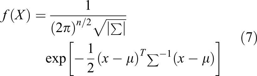
f (X) = \frac{1}{{(2 π)}^{n / 2} \sqrt{| \sum |}} \exp [- \frac{1}{2} {(x - μ)}^{T} \sum^{- 1} (x - μ)]

where μ is the mean vector and Σ is the covariance matrix with element c_{i, j} (1 ≤ i, j ≤ n) that can be expressed as

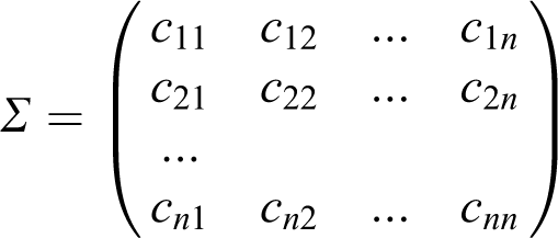
Σ = (\begin{matrix} c_{11} & c_{12} & ... & c_{1 n} \\ c_{21} & c_{22} & ... & c_{2 n} \\ ... \\ c_{n 1} & c_{n 2} & ... & c_{n n} \end{matrix})

It can be seen that the MVN density function is uniquely determined by the mean vector μ and covariance matrix Σ. The dependence structure is summarized in the covariance matrix Σ and zero correlation implies independence. The main shortcomings of the MVN are that it only measures the linear dependence and, in reality, the normal distribution may not be valid for the data at hand. Due to limitations of the linear correlation coefficient in characterizing the dependence, the MVN may not be suitable for certain applications, especially when far more complicated dependence structures are observed. To make the normal assumption valid, several techniques have been used for transforming non-normal multivariate data to approximately multivariate normal before working with the MVN, such as log transformation, power transformation, trigonometric transformation, and normal quantile transformation (NQT) (Bogner et al., 2012; Wang et al., 2009; Wilks, 2011). Due to the mathematical convenience and computational efficiency (particularly in high dimensions), the MVN distribution framework is still a popular choice in certain applications (Wilks, 2011).

3.2 Multivariate parametric distribution with flexible marginals

The fixed form of the marginal distribution has restricted the application of commonly used parametric distributions in hydrology and water resources. Several parametric methods have been developed that allow for flexible marginal distributions as well as dependence structures, among which the Farlie–Gumbel–Morgenstern and meta-Gaussian models have been commonly used.

For two continuous random variables X ₁ and X ₂ with marginal distributions F ₁(X ₁) and F ₂ (X ₂), the Farlie–Gumbel–Morgenstern bivariate density function f(x ₁, x ₂) can be expressed as (Long and Krzysztofowicz, 1992; Mari and Kotz, 2001; Singh and Singh, 1991)

f (x_{1}, x_{2}) = f_{1} (x_{1}) f_{2} (x_{2}) {1 + c ρ [F_{1} (x_{1}), F_{2} (x_{2})]}

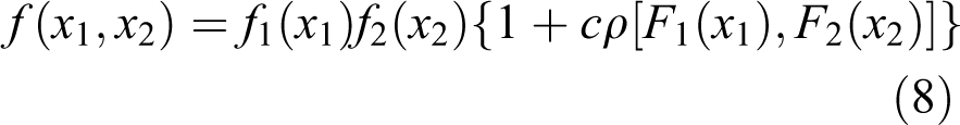
where c is a scalar and ρ is a kernel that models the dependence structure.

Although the Farlie–Gumbel–Morgenstern model allows for the arbitrary marginal distribution, it does not have wide applicability in hydrology, since only weak dependence or association can be modeled. One of the pioneering works in dependence modeling with the flexible marginal distributions is the meta-Gaussian model (Kelly and Krzysztofowicz, 1997), which represents a full range of associations.

The meta-Gaussian distribution function P(X, Y) for two continuous random variables X ₁ and X ₂ can be expressed as (Kelly and Krzysztofowicz, 1997)

P (X, Y) = N_{2} {Q^{- 1} [F (X_{1})], Q^{- 1} [F (X_{2})]}

where F ₁(X ₁) and F ₂ (X ₂) are marginal distributions, N ₂ is the bivariate standard normal distribution, and Q ^–1 is the inverse of the standard normal distribution (commonly referred to as the NQT).

The NQT is used to transform individual variables into normal variables, from which the MVN can be used to model the joint distribution of multivariate variables. Thus, the extension of the meta-Gaussian model to higher dimensions is fairly straightforward. The meta-Gaussian model has been used in dependence modeling for a variety of purposes, such as uncertainty estimation (Montanari and Brath, 2004; Montanari and Grossi, 2008) and probabilistic precipitation or river stage forecasting (Herr and Krzysztofowicz, 2005; Krzysztofowicz, 2002; Krzysztofowicz and Herr, 2001; Wu et al., 2011). The distinctive property of the meta-Gaussian model is that it can represent a full range of association between random variables with arbitrarily specified marginal distributions. The concepts of these parametric models in constructing the joint distribution with flexible marginals are closely related to the copula family that will be introduced afterwards.

IV Entropy

Entropy is a measure of uncertainty of random variables and has been used in a variety of areas in hydrology (Singh, 1997, 2011, 2014, 2016), including probability inference (Hao and Singh, 2013c; Papalexiou and Koutsoyiannis, 2012), streamflow simulation (Hao and Singh, 2011), parameter estimation (Hao and Singh, 2009; Singh, 1998), frequency analysis (Hao and Singh, 2013a), and geo-statistical modeling (Hou and Rubin, 2005; Singh, 2015; Woodbury and Ulrych, 1996), to name but a few. Entropy theory provides a criterion for statistical inference of probability distributions on the basis of partial knowledge, leading to the maximum entropy distribution that is a least biased estimate based on the given information (Jaynes, 1957a, 1957b). It has been shown that many of the commonly used parametric distributions, such as normal distribution and gamma distribution, can be derived based on the principle of maximum entropy (or minimum relative entropy), which can also be used for the derivation of multivariate distribution families for the modeling of multivariate data with certain dependence structures (Hao and Singh, 2013a; Kapur, 1989).

For a random variable X defined on the interval [a, b] with the probability density function (PDF) f(x), the Shannon entropy E can be defined as (Shannon, 1948; Shannon and Weaver, 1949)

E = - \int_{a}^{b} f (x) \ln f (x) d x

Based on the principle of maximum entropy, it is stated that the distribution with the maximum entropy, subject to specified constraints (or partial knowledge), should be selected. For a random vector with random variables X and Y on the interval [a, b] and [c, d] with the joint density function f(x, y), the entropy in the bivariate case E’ can be defined as (Kapur, 1989)

E ’ = - \int_{c}^{d} \int_{a}^{b} f (x, y) \ln f (x, y) d x d y

To infer the probability distribution f(x, y), a set of constraints have to be specified to model certain features of the data. With suitable specification of constraints, such as moments, L-moments, or pair-product, the entropy theory provides a flexible way of constructing the joint distribution to model different properties of the data, such as mean, standard deviation, skewness, or order statistics (Hao and Singh, 2011; Hosking, 2007; Kapur, 1989).

The general formulation of constraints can be expressed as

\int_{c}^{d} \int_{a}^{b} g_{i} (x, y) f (x, y) d x d y = E [g_{i} (x, y)] \begin{matrix}  \end{matrix} i = 0, 1, ..., m

where g_i (x, y) is the function of random variables x and y and E[g_i (x, y)] is the corresponding expectation.

The maximum entropy distribution can then be derived by maximizing the entropy in equation (11), subject to constraints in equation (12), as

f (x, y) = \exp [- \sum_{i = 0}^{m} λ_{i} g_{i} (x, y)]

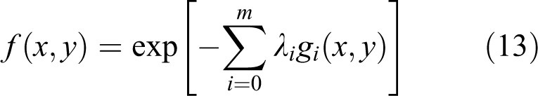
where λ_i (i = 0,1,., m) are the Lagrange multipliers.

The expression of the maximum entropy distribution in equation (13) depends on the specified constraints. With suitable choices of the function g(x, y) (e.g. cross term x and y), certain dependence structures can be modeled. For example, it has been shown that the Pearson correlation coefficient can be modeled pretty well when the moments for each variable and product moment are specified as the constraint (Hao and Singh, 2011).

A variety of multivariate distributions, such as MVN and multivariate Pearson’s type II distribution, can be derived with the entropy theory (Ebrahimi et al., 2008; Kapur, 1989). Note that the multivariate distribution constructed from the entropy is capable of modeling the data with different marginal distributions. In addition, the extension of the maximum entropy distribution to even higher dimensions is straightforward. The potential challenges of the maximum entropy distribution in modeling the dependence would be the modeling of marginal distributions and that of dependence structures not being separated, since the Lagrange multiplier associated with the dependence structure will also affect marginal distributions and vice versa. Since various dependence structures can be modeled by specifying suitable constraints with different marginal distributions, it is expected that more applications of entropy-based multivariate models in hydrology, such as rainfall simulation or downscaling, may be explored in the future.

V Copula

With the advent of the copula, recent years have witnessed a flurry of copula applications of dependence modeling in hydrology and water resources, such as frequency analysis (Favre et al., 2004; Hao and Singh, 2013a; Salvadori and De Michele, 2010), streamflow simulation or disaggregation (Hao and Singh, 2013b; Li et al., 2013), drought characterization (Hao and Singh, 2015a; Hao et al., 2014; Kao and Govindaraju, 2010), geo-statistical interpolation (Bardossy and Li, 2008), bias correction (Mao et al., 2014; Piani and Haerter, 2012; Vogl et al., 2012), error or uncertainty analysis (AghaKouchak et al., 2010a, 2010b; Chowdhary and Singh, 2010; Villarini et al., 2008), downscaling (Laux et al., 2011; Van den Berg et al., 2011; Verhoest et al., 2015), and statistical forecasting (Khedun et al., 2014). The copula provides a flexible method for constructing the joint distribution by separating the construction into two components: marginal distributions of individual variables and the interdependency of marginals. The main advantage of the copula method is that the construction of the joint distribution to modeling the dependence structure is independent of marginal distributions, which is the distinctive feature as compared with multivariate parametric distributions.

Let the marginal distribution of the continuous random vector (X, Y) be F_X (x) (denoted as U) and F_Y (y) (denoted as V). Based on Sklar’s theorem, the joint distribution function of the random vector (X, Y) can be expressed with a copula C as (Nelsen, 2006)

P (X \leq x, Y \leq y) = C [F_{X} (x), F_{Y} (y); θ] = C (u, v; θ)

where θ is the parameter of the copula, which represents the dependence structure. Copula C satisfies several properties, including C(u,0) = 0 = C(0, v), C(u,1) = u and C(1, v) = v. In the bivariate case, copula C in equation (14) maps the marginal distributions into the joint distribution as [0,1]² → [0,1].

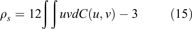
Certain dependence measures are directly linked to the copula function. For example, the Spearman rank correlation coefficient (ρ_s ) in equation (2) can be expressed with the copula function C(u, v) as

ρ_{s} = 12 \underset{}{} u v d C (u, v) - 3

In addition, the tail dependence can also be expressed with the copula function. Based on equations (5) and (6), the upper and lower tail dependences coefficient (λ_U and λ_L ) of multivariate random variables can be expressed as

λ_{U} = \lim_{t \to 1} \frac{1 - 2 t + C (t, t)}{1 - t}

λ_{L} = \lim_{t \to 0} \frac{C (t, t)}{t}

A variety of copula families are available to model various dependence structures (e.g., positive and negative dependence, symmetric and asymmetric dependence, tail dependence) of multivariate random variables, including, but not limited to, empirical copula, meta-elliptical copula, Archimedean copula, extreme value copula, vine copula, entropy copula, and others, each with its own merits (Hao and Singh, 2015b; Joe, 1997; Nelsen, 2006; Patton, 2012). The introduction of the copula in this section is confined to materials mostly related to properties of different types of copulas in dependence modeling (Figure 1).

Figure 1.

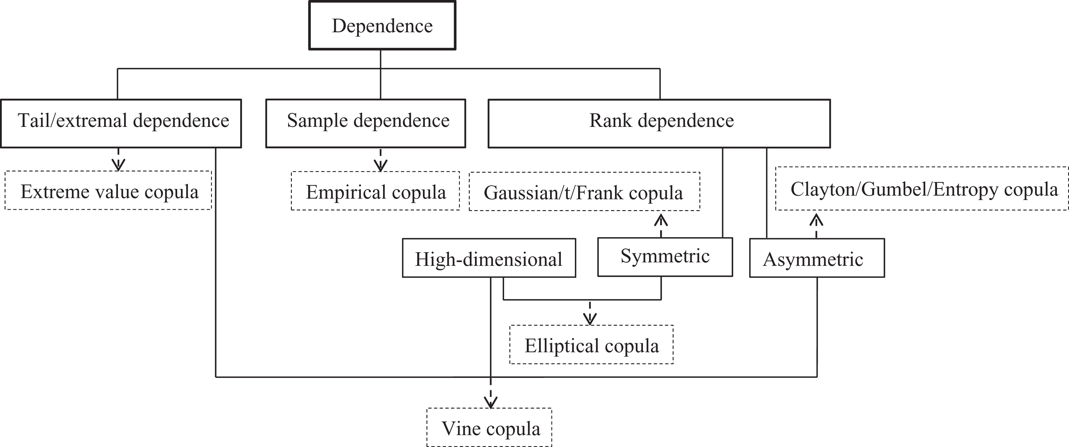
Modeling different dependence structures with copulas.

5.1 Empirical copula

The copula in equation (14) can be estimated empirically. Let (x_k , y_k ), k = 1,2,…, n, be the sample of size n. The empirical copula C_n can be expressed as (Nelsen, 2006)

C_{n} (\frac{i}{n}, \frac{j}{n}) = \frac{# (x \leq x_{(i)}, y \leq y_{(j)})}{n}

where x _(i) and x _(j) (1 ≤ i, j ≤ n) are order statistics of the sample.

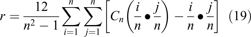
The empirical copula itself is a characterization of the dependence. It has been shown that the sample version of the Spearman and Kendall correlation coefficients can be expressed based on the empirical copula. For example, the sample version of the Spearman correlation coefficient can be expressed as (Nelsen, 2006)

r = \frac{12}{n^{2} - 1} \sum_{i = 1}^{n} \sum_{j = 1}^{n} [C_{n} (\frac{i}{n} • \frac{j}{n}) - \frac{i}{n} • \frac{j}{n}]

The empirical copula is essentially the sample representation of the copula. When used for modeling dependence, it has the advantage that it does not rely on the assumption of a specific copula family. When the underlying copula is not known in advance, the empirical copula can be employed for the dependence modeling of the data at hand, as witnessed in several applications, such as bias correction, downscaling, and uncertainty quantification (Laux et al., 2011; Piani and Haerter, 2012; Schefzik et al., 2013). However, unless enormous numbers of observations are available, it may lead to large errors in the extrapolation.

5.2 Parametric copula

The parametric copulas are important alternatives to the empirical copula introduced before. There are several families of parametric copulas, including the meta-elliptical copula (Gaussian and Student’s t), Archimedean copula (Clayton, Gumbel, Frank, Joe, and Ali-Mikhail-Haq), extreme value copula (Galambos copula, extremal-t copula, and Hüsler–Reiss copula), and other families (e.g. Plackett family) (Genest and Favre, 2007; Hao and Singh, 2015b; Nelsen, 2006). An important step in employing the parametric copula for dependence modeling is the selection of the suitable parametric copula that best fit the data. The empirical copula is commonly used to visualize the scatter plot of the data to aid the selection of copula families. Otherwise, the goodness-of-fit test statistics, such as the Cramér–von Mises statistic (S_n ) and the Kolmogorov–Smirnov statistic (T_n ), can be employed to select suitable copula functions (Genest et al., 2006).

The parametric copula is generally indexed by one or two parameters that control the strength of dependence among marginals. For example, the one-parameter Archimedean copulas have received much attention owing to their good properties, especially at the bivariate level (Hao and AghaKouchak, 2013; Kao and Govindaraju, 2008; Pan et al., 2013). The bivariate Archimedean copula C can be expressed as (Genest and Favre, 2007)

C (u, v; θ) = ϕ [ϕ^{- 1} (u) + ϕ^{- 1} (v); \begin{matrix}  \end{matrix} θ]

where ϕ is a convex and decreasing function (ϕ(1) = 0) known as the generator of the copula, from which different copulas can be identified (e.g. Clayton, Gumbel, Frank) and θ is the parameter embedded within the generator function ϕ.

Different types of copulas show distinctive properties in modeling various dependence structures. The Gaussian and t copulas of the elliptical copula family present the symmetric dependence. The Gaussian copula is capable of modeling the full range of dependence (both positive and negative) but does not account for the tail dependence (e.g. for the bivariate Gaussian copula, λ_U = λ_L = 0 for any correlation coefficient –1 < ρ < 1, i.e. no tail dependence unless ρ = 1). The non-Gaussian copula is required when the modeling of tail dependence is desirable. The Student’s t copula does allow for the dependence in the tails of the distribution but its tail dependence is symmetric. The Archimedean copula can take on various forms of distribution functions and is capable of modeling different upper and lower dependences. Specifically, the Frank copula exhibits symmetric dependence (similar to the Gaussian and Student’s t copulas) and can be used to model positive or negative dependence, which is most appropriate for modeling weak tail dependence. The Clayton copula exhibits strong left tail dependence and weak right tail dependence, while the Gumbel copula exhibits strong right tail dependence and relatively weak left tail dependence, both of which permit asymmetric dependence but generally do not account for negative dependence (Trivedi and Zimmer, 2005).

For dependence modeling in high dimensions, parametric copulas generally fall short in this regard. Although the Gaussian or t copulas are popular choices in high dimensions, a major drawback is the restrictive form of the symmetric dependence associated with elliptical copulas. The skew t copulas can partly address this issue by capturing asymmetric dependence and also be used in high-dimension dependence modeling (Demarta and McNeil, 2005; Smith et al., 2012). The Archimedean copula can also be extended to include additional marginal distributions or variables. However, it is generally restrictive in modeling the dependence of variables. For example, the trivariate Archimedean copula with marginals u, v, and w can be extended from equation (20) as

C (u, v, w; θ) = ϕ^{} [ϕ^{- 1} (u) + ϕ^{- 1} (v) + ϕ^{- 1} (w); θ]

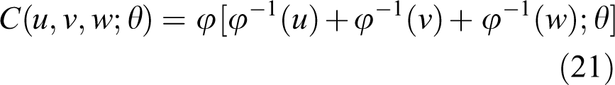
It can be seen that it unrealistically imposes the same dependence on different pairs of variables due to the single dependence parameter θ, which is the main drawback in the dependence modeling in high dimensions with the Archimedean copula. Several trivariate (or higher dimension) copula families exist for modeling dependence structures on different pairs of variables, such as the Plackett family copula (Kao and Govindaraju, 2008), meta-elliptical copulas (Fang et al., 2002; Genest et al., 2007; Song and Singh, 2010), and nested Archimedean construction (Grothe and Hofert, 2015; Joe, 1997; Xu et al., 2015). Nonetheless, overall dependence modeling with the multivariate parametric copula in higher dimensions is a difficult task to tackle and is generally limited in the range of dependence structures it can handle.

The advantages of standard parametric copulas are that generally one or two parameters need to be estimated to model different dependence structures. However, the assumption of a specific parametric copula function may be the potential drawback. A possible way out is to use the empirical copula in cases when the sample size is relatively large. In addition, the commonly used standard parametric copulas also suffer from the insufficiency of flexible dependence modeling (e.g. extreme dependence), especially in high dimensions, which will be partly addressed with the extreme value copula, vine copula, and entropy copula introduced in the following sections.

5.3 Extreme value copula

Although a variety of parametric copulas can be used for dependence modeling, they may not be suitable for cases when the dependence in the tail is of particular interest. The extreme value copula can be used for constructing the joint distribution with a focus on extreme values and provides a convenient way to model the dependence structure of rare events or extreme values (Bücher and Segers, 2014; Durante and Salvadori, 2010; Gudendorf and Segers, 2010; Salvadori et al., 2007).

A copula C is called the extreme value copula if there is a copula C_F such that (Gudendorf and Segers, 2010)

C_{F} {(u_{1}^{1 / n}, ..., u_{d}^{1 / n})}^{n} \to C (u_{1}, ..., u_{d})

where C_F is said to be in the domain of attraction of copula C.

For example, the Gumbel–Hougaard copula is an extreme value copula that is expressed as

C (u_{1}, ..., u_{d}) = \exp {- {[{\sum_{i = 1}^{d} (- \log u_{i})}^{1 / α}]}^{α}}

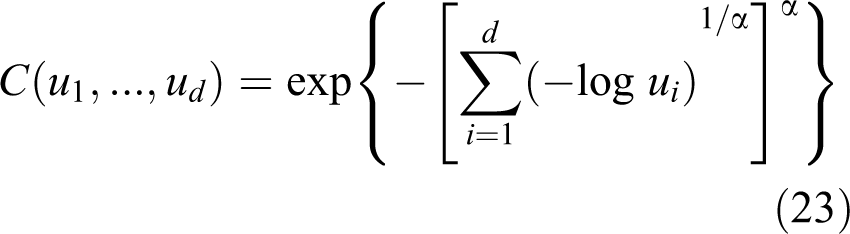
where α is the parameter with 0 < α ≤ 1 that characterizes the dependence structure. The Gumbel–Hougaard copula is the only extreme value copula that also belongs to the Archimedean copula.

Only a few of the copula families are extreme value copulas that can be used for multivariate extreme value modeling. The commonly used extreme value copulas include the Gumbel–Hougaard copula, Galambos (or negative logistic) copula, extremal-t copula, and Hüsler–Reiss copula (Gudendorf and Segers, 2010; Ribatet and Sedki, 2013). The first two copulas are generally limited for relatively high-dimension problems, since the dependence structure is characterized by a single parameter, while the extremal-t copula and Hüsler–Reiss copula do not suffer from this drawback of dependence modeling, and are easily generalized to infinite dimensional setting for stochastic process modeling, such as spatial extremes (Ribatet and Sedki, 2013; Wadsworth and Tawn, 2012). The past decade has seen many advances toward extreme value copula for the dependence modeling of hydroclimatic extremes for applications such as frequency analysis (Poulin et al., 2007; Serinaldi, 2013) and rainfall simulation (Davison et al., 2012). With the potential increase of extremes due to climate change, the extreme value copula is expected to be further explored to aid the dependence modeling of multivariate extremes or their properties.

5.4 Vine copula

The standard parametric copula suffers from the drawback of dependence modeling in high dimensions (Brechmann and Schepsmeier, 2013). To overcome some of the limitations of the standard parametric copula and facilitate the flexible dependence modeling in higher dimensions (Joe, 2014; Joe et al., 2010), the vine copula (or pair copula construction) has been recently developed (Bedford and Cooke, 2001; Cooke et al., 2015; Kurowicka and Cooke, 2006). A d-vine copula is a graphical model that is constructed from a set of d(d–1)/2 bivariate copulas via successive mixing according to a tree structure of d nodes, acting on two variables at a time (Bedford and Cooke, 2002). Depending on the type of trees, various copulas can be constructed, such as the C-vine and D-vine.

A multivariate density function can be expressed with the conditional distribution function. For the trivariate case of three random variables X ₁, X ₂, and X ₃ with marginal density functions f ₁(x ₁), f ₂(x ₂), and f ₃(x ₃), the joint density function can be expressed as

f (x_{1}, x_{2}, x_{3}) = f_{3} (x_{3}) \cdot f (x_{2} | x_{3}) \cdot f (x_{1} | x_{2}, x_{3})

where f (x _2| x ₃) is the conditional density of x ₂ given x ₃, and f ₁(x ₁|x ₂, x ₃) is the conditional density of x ₁ given x ₂ and x ₃.

By mathematical manipulation, it can be shown that the multivariate density function in equation (24) can be expressed as (Aas et al., 2009)

f (x_{1}, x_{2}, x_{3}) = f_{1} (x_{1}) \cdot f_{2} (x_{2}) \cdot f_{3} (x_{3}) \cdot c_{12} [F_{1} (x_{1}), F_{2} (x_{2})] \cdot c_{23} [F_{2} (x_{2}), F_{3} (x_{3})] \cdot c_{13|2} [F (x_{1} | x_{2}), F (x_{3} | x_{2})]

where c ₁₂[F ₁(x ₁), F ₂(x ₂)] and c ₂₃[F ₂(x ₂), F ₃(x ₃)] are the copula density functions and c _13|2[F ₁(x _1| x ₂), F ₃(x ₃|x ₂)] is the copula density function of X ₁ and X ₃ given X ₂. Note that there are different compositions of the multivariate density function in equation (25).

The vine copula decomposes the high-dimensional multivariate density into bivariate copulas in which low-dimension integrals are involved. Through decomposition, it allows for the selection of different bivariate copulas for the modeling of flexible dependence structures among different pair variables. For example, the dependence between X ₁ and X ₂ can be modeled with the bivariate copula density c ₁₂[F ₁(x ₁), F ₂(x ₂)], while the dependence between X ₂ and X ₃ can be modeled with another copula density c ₂₃[F ₂(x ₂), F ₃(x ₃)]. In addition, the vine copula also enables the modeling of flexible tail dependence, which stems not only from flexible parametric families of cascade bivariate copulas, but also the underling graphical (or tree) structures (Joe et al., 2010). Overall, compared with the commonly used standard parametric copula, the distinct advantage of the vine copula is its flexibility in modeling the dependence structure, including the tail dependence, even in high dimensions (Aas et al., 2009; Joe, 2014; Kurowicka and Joe, 2011). Although the vine copula has emerged to be used in several hydrologic studies, such as rainfall simulation and frequency analysis (Gräler et al., 2013; Gyasi-Agyei, 2011; Gyasi-Agyei and Melching, 2012; Vernieuwe et al., 2015; Xiong et al., 2014), application of the vine copula in hydrology and water resources is rather limited and there is great potential in exploring the vine copula to aid dependence modeling in applications such as uncertainty estimation, downscaling, and statistical forecasting, where other copulas have been extensively explored.

5.5 Entropy copula

Entropy has been introduced as one way to derive the multivariate distribution to model the dependence as introduced before. Following similar procedures, the principle of maximum entropy (and minimum cross-entropy) can also be used to infer the copula function when no prior information about the distribution function is available. In the following, the copula derived from entropy theory (termed as the entropy copula) in the continuous form is introduced to model the dependence structure (Hao and Singh, 2012, 2013b, 2015b).

By denoting the copula density function as c(u, v), the entropy of the copula density function E_c can be expressed as (Chu, 2011; Chui and Wu, 2009)

E_{c} = - \int_{0}^{1} \int_{0}^{1} c (u, v) \ln c (u, v) d u d v

As introduced in the previous section, a set of constraints has to be specified to infer the copula density c(u, v). The general expression of the constraints for the copula density function c(u, v) can be expressed as

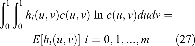
\int_{0}^{1} \int_{0}^{1} h_{i} (u, v) c (u, v) \ln c (u, v) d u d v = E [h_{i} (u, v)] \begin{matrix}  \end{matrix} i = 0, 1, ..., m

where h_i (x, y) is the constraint function and E[h_i (x, y)] is the corresponding expectation.

With the constraints specified as above, the maximum entropy copula can be expressed as (Chu, 2011; Hao and Singh, 2013b)

c (u, v) = \exp [- \sum_{i = 0}^{m} λ_{i} h_{i} (u, v)]

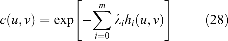
where λ_i (i = 0,1,., m) are the Lagrange multipliers.

Through appropriate specifications of the constraint function h(u, v), certain commonly used dependence measures can be modeled. For example, by specifying h(u, v) = uv, the Spearman rank correlation can be modeled. Other dependence measures, such as Blest’s measure and Gini’s measure, can also be modeled by suitably specifying the function h(u, v) (Chu, 2011; Hao and Singh, 2015b). This can be extended to even higher dimensions to model temporal and spatial dependences, such as monthly streamflow among different sites (Hao and Singh, 2013b).

The dependence modeling with the entropy copula can be achieved through the selection of suitable constraints to represent the dependence structure in the data. The advantages of the entropy copula are that the modeling of marginal distributions and dependence structure can be separated and it is straightforward to be extended to the high dimension. However, the computation burden due to the relatively large number of Lagrange multipliers would be the potential challenge in the application (similar to the multivariate entropy distribution). Up to now, there have only been limited applications in hydrology, such as frequency analysis (Hao, 2012), streamflow simulation (Hao and Singh, 2013b), and rainfall simulation (Piantadosi et al., 2012). With the derivation of the copula based on the entropy theory, various new copulas can be obtained to model the dependence structure of hydrologic variables. It is expected that the entropy copula may be applied in other applications when the dependence modeling is desired, such as bias correction and downscaling.

VI Nonparametric methods

One limitation of parametric methods in statistics is that certain assumptions about the distribution forms of data (e.g. Gaussian) and dependence structure (e.g. linear dependence) have to be made. However, in reality, hydrological variables may exhibit a variety of features, such as bimodality, skewness, tail properties, and complex dependence structures, which are not easily captured by limited families of parametric distributions that are indexed by a set of parameters and prescribed function forms (Sivakumar and Berndtsson, 2010). Nonparametric models have been commonly used for modeling rich features of the data (Härdle et al., 1997; Lall, 1995; Scott, 1992; Silverman, 1986), which have been widely used to model complex dependence structures of hydrologic variables for various applications, such as streamflow simulation (Prairie et al., 2007; Salas and Lee, 2010; Sharma and O’Neill, 2002; Tarboton et al., 1998), downscaling (Gangopadhyay et al., 2005; Kannan and Ghosh, 2013; Lu and Qin, 2014), rainfall simulation (Buishand and Brandsma, 2001; Rajagopalan and Lall, 1999; Rajagopalan et al., 1997; Yates et al., 2003), and statistical forecasting (Souza Filho and Lall, 2003). The advantages are that they are mostly free from assumptions about the data and are capable of preserving complex dependence structures and distribution properties of observations, allowing the data to speak for themselves. Typical nonparametric methods include the kernel density estimation and the K-nearest neighbor (KNN) estimation.

6.1 Kernel density estimation

The kernel density estimation generalizes the concept of the histogram for the probability density estimation by centering a smooth kernel function at each observation. For a random vector, the multivariate case of the kernel density estimator in d dimension can be expressed as (Scott, 1992)

f (X) = \frac{1}{n h^{d}} \sum_{i = 1}^{n} K (\frac{X - x_{i}}{h})

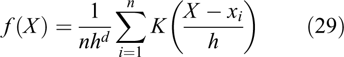
where n is number of observations, h is the bandwidth that defines how the empirical frequency distribution is smoothed or averaged, and K(.) is a kernel function that is usually symmetric and uni-modal that satisfies

\int_{}^{} K (x) d x = 1

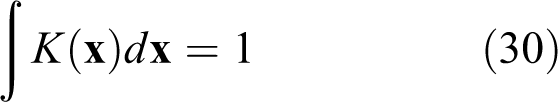
There are a variety of kernel functions, such as Gaussian, quadratic, and bisquare functions, which can be used to derive the joint distribution for dependence modeling. In a multivariate setting, the product kernel and sphering kernel are popular choices (Lall and Bosworth, 1994). It has been recognized that in estimating the density function f(X), the optimal bandwidth h is more crucial than the choice of the kernel function K and different kernels can be made equivalent under rescaling through appropriate bandwidths (Rajagopalan et al., 2010; Sivakumar and Berndtsson, 2010).

6.2 K-nearest neighbor estimation

The main drawback of the kernel density estimation is its inability to handle satisfactorily the tail distributions without over-smoothing the main body of the density (or the boundary problems; Silverman, 1986). In the multivariate case, boundary problems would get worse, leading to biases in the density estimation and simulation (Rajagopalan et al., 2010). The KNN estimation provides a flexible and robust alternative that partly overcomes the drawbacks of traditional kernel density estimation. For a random vector X, the KNN density estimation in the multivariate case can be expressed as (Rajagopalan et al., 2010)

f (X) = \frac{1}{n r_{k}^{d} {(X)}^{}} \sum_{i = 1}^{n} K [\frac{X - x_{i}}{r_{k} (X)}]

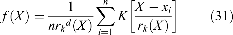
where k is the number of nearest neighbors (or the smoothing parameter), r_k is the Euclidean distance to the kth nearest neighbor, and K(.) is a kernel function.

Although measures such as the rank correlation are generally used to depict the dependence, in many cases the dependence inherent in sample data cannot be fully characterized by these parameters. The nonparametric density estimation is essentially the weighted moving average in the neighborhood around the point of estimation, which provides the “local” estimate of the target density function (Lall and Bosworth, 1994). Consequently, the dependence is generally estimated locally through the kernel in the multivariate distribution construction and complex dependence structures, including the linear and nonlinear dependences, of samples from historical records can be modeled or preserved. However, the nonparametric method is data driven and thus requires a relatively long data record for accurate estimation. In addition, due to the boundary problem, limitations exist such as the difficulty in the extrapolation and reproduction beyond historical observations, which may restrict its application in certain applications such as frequency analysis. To alleviate these drawbacks, parametric and nonparametric methods have been integrated (or the semi-parametric method, hybrid method) that provide attractive alternatives to combine advantages of both methods for modeling multivariate variables (Apipattanavis et al., 2007; Rajagopalan et al., 2010).

VII Discussion

7.1 Strength and limitation

Considering various methods available for dependence modeling, it is important to be aware of distinct properties of each method to aid the selection of the most suitable method for the specific context of applications. Multivariate parametric distributions are the classical methods for modeling the joint behavior of multivariate random variables, which are generally extended from the univariate distribution. Their wide applications are hindered by properties that parameters of the marginal distribution may mix up with the dependence structure and extensions of the multivariate distribution to higher dimensions are rather limited (or not clear). Multivariate parametric distributions are still popular in dependence modeling, in many cases mainly due to their simplicity or mathematical convenience (e.g. MVN).

Entropy theory provides a criterion for the inference of multivariate distributions for dependence modeling through the principle of maximum (or minimum relative) entropy. The construction of multivariate distributions for dependence modeling may incorporate different marginal distributions and the extension to high dimensions is straightforward. However, the dependence modeling with the entropy method is not separate from the modeling of marginal distributions. Since the entropy-based multivariate distributions can be constructed with different marginal distributions to model rich features of the data, it is expected that the entropy method may be applied in more applications, such as weather generators or downscaling in the future.

The copula method has surged in applications of dependence modeling of multivariate hydroclimatic variables in the past decade. It enables one to model marginal distributions and joint distributions (or dependence structures) separately, which makes it a widely used method in the dependence modeling for various applications in hydrology and water resources. A suite of copula families, including the empirical copula, parametric copula, extreme value copula, vine copula, and entropy copula, are available, which allow for the modeling of rank correlation and tail (or extreme) dependence. In many cases, the goodness-of-fit tests, such as the Cramér–von Mises statistic and the Kolmogorov–Smirnov statistic, can be used for testing the hypothesis of a suitable copula function, especially in the bivariate case. However, it is unclear as to what to do when all the candidates are rejected. In this case, the empirical copula provides useful alternatives to construct a suitable copula model for dependence modeling without making assumptions about the distribution form. The commonly used parametric copulas, such as the Gaussian copula, may fall short in describing the tail (or extreme) dependence. The extreme value copula is a suitable model when the dependence in the tail (or extreme) region is of primary concern or interest. The dependence modeling with the bivariate copula is generally well understood. However, the modeling of dependences in high dimensions is a challenge for the standard copula families. With the recent development of the vine copula showing a great advantage in flexible dependence modeling (including tail dependence), it is expected that extensive applications of the vine copula may be witnessed in the future. When no prior information is available, the copula derived from the entropy would be an interesting alternative from which new families of copulas can be obtained.

The nonparametric method provides an attractive alternative in dependence modeling and is preferable when assumptions required for parametric methods are not valid. It lets the data speak for themselves and is capable of preserving the dependence in the original data. The main drawback of the nonparametric method includes the boundary problem, which may hinder the extrapolation or simulation beyond the historical range. In addition, as a data-driven method, it generally requires a relatively long data record for suitable modeling of the data at hand. As such, it is less favorable when the extrapolation is required or when the sample size of the observation is relatively small. The combination of the nonparametric method with the parametric methods provides useful alternatives for dependence modeling that may alleviate the potential drawbacks of the nonparametric method.

7.2 Temporal and spatial dependence

Temporal and spatial dependences are important topics in the dependence modeling, for which methods introduced above for the dependence across random variables can be used with variations for applications in hydrology and water resources. The temporal (or serial) dependence is related to the dependence modeling of an individual variable or multiple variables in a stochastic process, which is generally cast as hydrological time series analysis. The parametric ARMA framework is commonly used for the temporal dependence modeling, which is based solely on the linear correlation of lagged observations (Brockwell and Davis, 1991; Hipel and McLeod, 1994; Machiwal and Jha, 2012; Salas et al., 1985). One distinct shortcoming is that only the linear dependence among hydrologic variables can be modeled due to the Gaussian assumption. To overcome this drawback, methods such as copula and nonparametric methods have been used for modeling the nonlinear serial dependence of hydrologic variables by constructing the corresponding joint or conditional distributions. Although the copula has been recently used to construct the first-order or higher order Markov processes for modeling the nonlinear serial dependence mainly in econometrics and finance (Abegaz and Naik-Nimbalkar, 2008; Beare and Seo, 2014; Chen and Fan, 2006; Ibragimov, 2009; Patton, 2012), only limited applications for temporal dependence modeling in hydrology and water resources have been explored (Hao and Singh, 2013b; Serinaldi, 2009). Meanwhile, the nonparametric method (especially the KNN resampling approach) has also been used for the time series analysis for modeling the temporal dependence in hydrological applications, such as streamflow simulation and rainfall downscaling (Lall and Sharma, 1996; Mehrotra and Sharma, 2006; Rajagopalan et al., 2010), which is capable of modeling the nonlinear dependence based on the local estimation of the density function and the associated dependence (Sharma et al., 1997).

The spatial dependence is generally related to the dependence modeling of variables at multiple locations across a region. This is the common case in many hydrologic applications, such as statistical downscaling, streamflow simulation or disaggregation, weather generators, or geo-statistical modeling, in which, except for the statistical properties of a random variable at a single site, the suitable modeling of dependence of variables at different sites, with or without conditioning on exogenous atmospheric variables or predictors, is also required (Apipattanavis et al., 2007; Nowak et al., 2011; Srivastav and Simonovic, 2015; Wilks, 1998). Extending parametric models to the spatial dependence modeling of multiple sites is not trivial, since a major disadvantage is that the number of model parameters will grow exponentially with the number of locations (Caraway et al., 2014; Mehrotra et al., 2006). Except for the traditional ARMA framework, copula and nonparametric methods have also been commonly used for multi-site nonlinear dependence modeling for different applications (Bardossy, 2006; Bárdossy and Pegram, 2009; Ben Alaya et al., 2014; Hao and Singh, 2013b; Koutsoyiannis, 2000; Lee et al., 2010; Nowak et al., 2010; Serinaldi, 2009; Stedinger et al., 1985). In many cases, the temporal and spatial dependence may be modeled simultaneously, for which the dependence modeling in high dimensions is particularly desired, since the dependence modeling is not only among the same variables of different time steps/scales, but also among variables at multiple sites (Ailliot et al., 2015; Efstratiadis et al., 2014; Huser and Davison, 2014; Kleiber et al., 2012; Kyriakidis and Journel, 1999; Srikanthan and McMahon, 1999; Wilks and Wilby, 1999). While the dependence modeling in high dimensions is always a potential issue to tackle, the vine copula introduced before may find its way in related applications of temporal and/or spatial dependence modeling due to its ability in nonlinear and tail dependence modeling, especially in high dimensions.

7.3 Extreme dependence

Statistical modeling of extremes is commonly used for extrapolation beyond the range of observations to estimate probabilities of rare events, which is particularly important for water resources management and design (Hao and Singh, 2013c; Katz et al., 2002). The two principal kinds of models for extreme values, the generalized extreme value distribution and generalized Pareto distribution, which correspond to the approximate distributions of block maxima and threshold exceedance, respectively, based on the extreme value theory, have been commonly used for extreme modeling and analysis in the univariate case. In practice, risk analysis of extremes in hydrology generally requires the characterization of extreme events that are inherently multivariate (e.g. simultaneously large values of two or more variables), including flood and drought occurrences (Salvadori and De Michele, 2010), extreme rainfall and storms (Zheng et al., 2014), heat waves and droughts (Hao et al., 2013), and extreme rainfall at different sites (Davison et al., 2012; Thibaud et al., 2013). Multivariate extreme value analysis is related to extremes that at least some components have relatively large values. Interactions of physical processes leading to the multivariate (or compound, concurrent) extremes have been emphasized and the dependence modeling of multivariate extremes has been an active research field in past decades (Davison and Huser, 2015; Dutfoy et al., 2014; Field et al., 2012).

The boundary cases of the dependence structure of the multivariate extreme value distribution are the independence and complete dependence, in which the dependence of extremes generally lies, including the asymptotic dependence (large values of components tend to occur simultaneously at extreme levels) and asymptotic independence (components exhibit positively or negatively associations that gradually disappear at extreme levels; Beirlant et al., 2006; Eastoe et al., 2013). Traditional methods for dependence modeling may not be suitable for characterizing the dependence in extremes (or tails) of hydrologic variables, for which the multivariate extreme value models have been developed to model various dependence structures of extremes, either based on the component-wise maxima or multivariate threshold exceedances. However, unlike the univariate extreme, the class of multivariate extreme value (MEV) distributions cannot be represented by a parametric family of distributions indexed by finite dimensional parameters. Thus, several parametric subfamilies have been proposed to give simpler representations of the MEV distribution with a relatively wide range of dependence structures especially in the bivariate case, such as the negative logistic and bilogistic model (Beirlant et al., 2006; Kotz and Nadarajah, 2000). Recently, considerable efforts have been devoted to the development of the max-stable model and conditional extreme model to characterize different types of extreme dependences (Davison and Huser, 2015; Haan and Ferreira, 2006; Heffernan and Tawn, 2004; Jonathan and Ewans, 2013). While many MEV models assume a particular form of extremal dependence or restrict attention to regions where all variables are extreme, the recently developed conditional extreme model (Heffernan and Resnick, 2007; Heffernan and Tawn, 2004) can be used to model flexible dependence structures, including asymptotic dependence and asymptotic independence, when one variable is extreme while the other may not be extreme. Among the research upsurge in multivariate extreme modeling, there has been considerable interest in the field of spatial extreme modeling of hydroclimatic variables at different locations and the max-stable process, as an infinite dimensional generalization of the multivariate extreme value distribution, arises as the natural model for spatial extremes of maxima (Bacro and Gaetan, 2012; Cooley et al., 2012; Davison and Gholamrezaee, 2012; Davison et al., 2013; Huser and Davison, 2014; Wadsworth and Tawn, 2012). It is expected that the dependence modeling of multivariate extremes may be further explored in various applications to aid water resources planning and management owing to the potential increase of extremes due to effects of global climate change.

7.4 Dependence modeling in a changing climate

Traditional statistical analysis to assess the risk for engineering design is based on the assumption of a stationary climate. Climate change has altered the mean and extremes of hydroclimatic variables, such as precipitation, temperature, evapotranspiration, and river discharge (Field et al., 2012; IPCC, 2013). Consequently, the stationarity assumption should not serve as a central and default assumption in risk assessment and planning in hydrology and water resources (Milly et al., 2008, 2015), and non-stationary features have to be identified and modeled to facilitate engineering design in a changing climate (Borgomeo et al., 2014; Rootzén and Katz, 2013; Serinaldi and Kilsby, 2015). Several techniques, such as the inclusion of time-varying parameters, moments, or covariates (Du et al., 2015; Katz et al., 2002; Khaliq et al., 2006; Parey et al., 2010; Villarini et al., 2009; Zhang et al., 2015), have been used to reflect the changing climate factors. The non-stationary feature is an important factor to be taken into account in statistical modeling and may lead to substantial changes in the engineering design in hydrology under climate change. For example, when the non-stationary feature is incorporated in the frequency analysis, the non-exceedance probability of hydrologic variables of interest is not constant anymore and the estimation of return level (often termed as “effective return level” in this case) generally varies as a function of time (Cheng et al., 2014, 2015; Read and Vogel, 2015; Rootzén and Katz, 2013; Salas and Obeysekera, 2014).

However, most of the current studies of non-stationary modeling of hydroclimatic variables are focused on the univariate analysis of a particular variable, such as the precipitation or temperature (Coles, 2001; Cooley et al., 2007; Katz, 2010). Climate change affects not only the variability of hydroclimatic variables but also their dependence structures (Chebana et al., 2013; Hao and Singh, 2015b). As such, suitable statistical methods are required to incorporate non-stationary features not only in marginal distributions of individual variables, but also in the dependence structure (or both). Although the non-stationary property of individual variables can be taken into account with the methods introduced above, it is not straightforward to model the non-stationarity in the dependence structure. There have been rather limited studies on the dependence modeling in a non-stationary case in hydrology and, recently, modeling the non-stationarity of the dependence structure has been expanding with a few applications such as downscaling and return level estimation (or frequency analysis; Eastoe, 2009; Huser and Genton, 2014; Jiang et al., 2015; Jonathan et al., 2014a, 2014b; Salvi et al., in press; Wilks, 2012). For example, the non-stationary dependence structure of hydrological variables or properties can be modeled through the copula method with time-dependent copula parameters for flood frequency analysis (Bender et al., 2014). Overall, it is a challenge to model non-stationary features in the dependence structure and with the growing concern and attention of the impact due to climate change (or land use), dependence modeling with suitable methods taking into account non-stationary features for different applications would be an important topic to explore in the future.

7.5 Model selections

No multivariate distribution or family satisfies all desired dependence properties of the data of interest. The choice of different methods mostly depends on the context of the application with specific dependence type. For example, when the joint upper or lower dependence is of particular interest, the multivariate extreme models, such as the max-stable model and conditional extremes model, are generally suitable. For cases when a large number of variables are involved and nonlinear dependence modeling in high dimensions is desirable, the vine copula is among the most popular choices. Except for the dependence type and dimension property, there are several factors that may affect the selection of methods in dependence modeling. Marginal distributions play an important role in the choice of methods for dependence modeling of multivariate random variables. For example, in cases of complex marginal distributions, such as the mixture of distributions that is widely used to model the heterogeneous phenomena (Favre et al., 2004), the copula method is more appropriate due to the separation of the marginal and joint distribution modeling. Statistical extrapolation beyond observations is an important task for statistical analysis in hydrology and may also affect the choice of methods. For example, although mostly free from assumptions about the distribution form, the kernel density estimation method is generally not admissible for frequency analysis, since the issue with the boundary condition hinders it from extrapolation of probabilities beyond the range of observations (Lall, 1995). Moreover, mathematical convenience is an important factor in selecting methods for multivariate modeling, especially when there are no stochastic or physical mechanisms that lead to the specific model (Joe, 2014; Wilks, 2011). For example, although the parametric MVN suffers from the insufficiency of describing nonlinear dependence properties, the MVN-based framework has been widely used in a variety of cases. Finally, the choice of different methods also depends on the length of the data and, consequently, the empirical or nonparametric methods are generally not suitable when the sample size is relatively small.

7.6 Model applications

Dependence modeling plays a key role in a variety of applications in hydrology and water resources, where the statistical link between two groups of variables has to be established, including frequency analysis, streamflow (or rainfall) simulation and disaggregation, drought characterization, geo-statistical interpolation, bias correction, downscaling, error or uncertainty analysis, and statistical forecasting, to name a few. Let X and Y be two random variables representing hydroclimatic variables or associated properties. Since the dependence between random variables X and Y is completely described by their joint distribution function, the construction of the joint distribution F(X, Y) or conditional distribution F(Y|X) is the key to model the dependence between X and Y to facilitate a variety of applications (Figure 2), which can be achieved with the methods reviewed herewith. For example, for the multivariate frequency analysis, which is commonly used to assess the risk for engineering design, dependence between hydroclimatic variables (e.g. precipitation, streamflow, soil moisture) or their properties (e.g. drought duration and severity, rainfall duration and severity, flood volume and peak) have to be built. In this case with X and Y representing different variables or properties such as drought duration and severity, the joint distribution F(X, Y) or conditional distribution F(Y|X) can be constructed with the parametric model, entropy, or copula models to perform the joint or conditional drought frequency analysis. As another example, for statistical downscaling, which is commonly used to render the consistency of two data sources with difference scales or resolutions for applications such as assessing the hydrological impact of climate change, dependence between large-scale climatic variables (e.g. outputs from General Circulation Models (GCMs) or Regional Climate Models (RCMs)) and local-scale climatic or hydrologic variables has to be modeled. In this case with X representing a large-scale variable and Y representing a local-scale variable at a site or location, the conditional distribution F(Y|X) can be used to downscale the local variable Y conditioned on the variable X. Overall, a variety of applications introduced above can be formalized as the topic of exploring the dependence, which can be achieved and further explored with methods reviewed in this study. Theoretically, once the multivariate distribution of various forms of a feature vector of interest are identified, these methods can be used for a variety of applications in hydrology and water resources where dependence modeling is involved and the method development in each vein of the applications may benefit from other types due to the common feature of dependence modeling.

Figure 2.

Applications of dependence modeling of random variables (or vectors) with the multivariate distribution F(X, Y) or conditional distribution F(Y|X) in hydrology and water resources.

VIII Conclusions

Modeling hydrologic events exhibiting multivariate features inherently for water resources planning and management requires suitable models that account for various dependence structures (such as linear dependence, rank correlation, or tail dependence) of multivariate variables and properties. This review attempts to build a thread linking the commonly used methods for modeling dependence structures of multivariate variables in hydrology and water resources. Strengths and limitations of different methods are also provided to aid the model selection and application, along with suggestions for future research opportunities.

Recent advances in dependence modeling have mainly been in the improvement of nonlinear dependence modeling (e.g. rank correlation or tail dependence) with flexible marginal distributions. Dependence modeling of extremes in the multivariate setting is a rapidly advancing field that concerns the modeling and analysis of multivariate extremes and is expected to be an important topic to be further investigated concerning the potential increase of extremes with global warming. Modeling dependence of multivariate variables in high dimensions, which has been commonly encountered in temporal or spatial dependence modeling, represents a prevailing challenge due to the curse of dimensionality that may result in difficulties in model fitting, checking, and simulation. The development of vine copula construction with flexible dependence structures is among the greatest advances for high-dimensional copula models and applications in recent years (Joe et al., 2015), which may partly address the challenge of dependence modeling in high dimensions, and efforts are particularly needed in this regard to explore the implementation of the vine copula to aid applications in hydrology and water resources. Under the changing climate, how to develop and apply suitable models in dependence modeling to incorporate non-stationary features in the dependence structure for related applications is an outstanding challenge. With several methods available for modeling various dependence structures through the construction of the joint or conditional distribution, an associated challenge is the selection of a suitable method taking into account various factors, such as dependence type, dimension property, marginal distributions, extrapolation purpose, mathematical convenience, and data length, to facilitate accurate dependence modeling.

Due to wide applications of different methods for constructing multivariate distributions for dependence modeling, it is impossible to review all methods and developments in the space available. Here we have focused on the methods for deriving multivariate distributions to facilitate the modeling of various dependence structures that are of particular interest in hydrology and water resources. There are also other methods that can be used for dependence modeling for various applications, such as the regression method (Maraun et al., 2010; Wilks and Wilby, 1999; Yang et al., 2005). It is important to bear in mind that there is not a universal method that is suitable for all cases of dependence modeling in hydrology and water resources. The method emanating from this review is to balance the desired properties of an application with the strengths and weaknesses of specific methods. This study provides guidelines for modeling dependences of multivariate random variables with various statistical methods in hydrology for research and operational purposes and may aid the practices of dependence modeling for water resources planning and management.

Footnotes

Declaration of conflicting interests

The author(s) declared no potential conflicts of interest with respect to the research, authorship, and/or publication of this article.

Funding

The author(s) disclosed receipt of the following financial support for the research, authorship, and/or publication of this article: This work was supported by Youth Scholars Program of Beijing Normal University (Grant No. 2015NT02).

References

Aas

Czado

Frigessi

. (2009) Pair-copula constructions of multiple dependence. Insurance: Mathematics and Economics 44(2): 182–198.

Abegaz

Naik-Nimbalkar

(2008) Modeling statistical dependence of Markov chains via copula models. Journal of Statistical Planning and Inference 138(4): 1131–1146.

Adamson

Metcalfe

Parmentier

(1999) Bivariate extreme value distributions: an application of the Gibbs sampler to the analysis of floods. Water Resources Research 35(9): 2825–2832.

AghaKouchak

Bárdossy

Habib

(2010a) Copula-based uncertainty modelling: Application to multisensor precipitation estimates. Hydrological Processes 24(15): 2111–2124.

AghaKouchak

Habib

Bardossy

(2010b) Modeling radar rainfall estimation uncertainties: Random error model. Journal of Hydrologic Engineering 15(4): 265–274.

Ailliot

Allard

Monbet

. (2015) Stochastic weather generators: An overview of weather type models. Le Journal de la Société Française de Statistique 156(1): 101–113.

Apipattanavis

Podestá

Rajagopalan

. (2007) A semiparametric multivariate and multisite weather generator. Water Resources Research 43: W11401(11).

Bacchi

Becciu

Kottegoda

(1994) Bivariate exponential model applied to intensities and durations of extreme rainfall. Journal of Hydrology 155(1): 225–236.

Bacro

J-N

Gaetan

(2012) A review on spatial extreme modelling. In: Porcu

Montero

Schlather

(eds) Advances and Challenges in Space-time Modelling of Natural Events. New York: Springer, 103–124.

10.

Balakrishnan

Johnson

Kotz

(1994) Continuous Univariate Distributions. New York: Wiley, 752.

11.

Balakrishnan

Lai

(2009) Continuous Bivariate Distributions. New York: Springer, 688.

12.

Bardossy

(2006) Copula-based geostatistical models for groundwater quality parameters. Water Resources Research 42(11): W11416.

13.

Bardossy

(2008) Geostatistical interpolation using copulas. Water Resources Research 44: W07412.

14.

Bárdossy

Pegram

(2009) Copula based multisite model for daily precipitation simulation. Hydrology and Earth System Sciences 13(12): 2299–2314.

15.

Beare

Seo

(2014) Vine copula specifications for stationary multivariate Markov chains. Journal of Time Series Analysis 36(2): 228–246.

16.

Bedford

Cooke

(2001) Probability density decomposition for conditionally dependent random variables modeled by vines. Annals of Mathematics and Artificial intelligence 32(1–4): 245–268.

17.

Bedford

Cooke

(2002) Vines--A new graphical model for dependent random variables. The Annals of Statistics 30(4): 1031–1068.

18.

Beersma

Buishand

(2004) Joint probability of precipitation and discharge deficits in the Netherlands. Water Resources Research 40(12): W12508.

19.

Beirlant

Goegebeur

Segers

. (2006) Statistics of Extremes: Theory and Applications. Chichester: Wiley, 514.

20.

Ben Alaya

Chebana

Ouarda

TBMJ

(2014) Probabilistic Gaussian copula regression model for multisite and multivariable downscaling. Journal of Climate 27(9): 3331–3347.

21.

Bender

Wahl

Jensen

(2014) Multivariate design in the presence of non-stationarity. Journal of Hydrology 514: 123–130.

22.

Bogner

Pappenberger

Cloke

. (2012) Technical Note: The normal quantile transformation and its application in a flood forecasting system. Hydrology & Earth System Sciences 16(4): 1085–1094.

23.

Borgomeo

Hall

Fung

. (2014) Risk-based water resources planning: Incorporating probabilistic nonstationary climate uncertainties. Water Resources Research 50(8): 6850–6873.

24.

Brechmann

Schepsmeier

(2013) Modeling dependence with C-and D-vine copulas: The R-package CDVine. Journal of Statistical Software 52(3): 1–27.

25.

Brockwell

Davis

(1991) Time Series: Theory and Methods. New York: Springer, 580.

26.

Bücher

Segers

(2014) Extreme value copula estimation based on block maxima of a multivariate stationary time series. Extremes 17(3): 495–528.

27.

Buishand

Brandsma

(2001) Multisite simulation of daily precipitation and temperature in the Rhine basin by nearest-neighbor resampling. Water Resources Research 37(11): 2761–2776.

28.

Caraway

McCreight

Rajagopalan

(2014) Multisite stochastic weather generation using cluster analysis and k-nearest neighbor time series resampling. Journal of Hydrology 508: 197–213.

29.

Chebana

Ouarda

Duong

(2013) Testing for multivariate trends in hydrologic frequency analysis. Journal of Hydrology 486: 519–530.

30.

Chen

Fan

(2006) Estimation of copula-based semiparametric time series models. Journal of Econometrics 130(2): 307–335.

31.

Cheng

AghaKouchak

Gilleland

. (2014) Non-stationary extreme value analysis in a changing climate. Climatic Change 127(2): 353–369.

32.

Cheng

Phillips

AghaKouchak

(2015) Non-stationary return levels of CMIP5 multi-model temperature extremes. Climate Dynamics 44(11–12): 2947–2963.

33.

Chowdhary

Singh

(2010) Reducing uncertainty in estimates of frequency distribution parameters using composite likelihood approach and copula-based bivariate distributions. Water Resources Research 46: W11516.

34.

Chu

(2011) Recovering copulas from limited information and an application to asset allocation. Journal of Banking & Finance 35(7): 1824–1842.

35.

Chui

(2009) Exponential series estimation of empirical copulas with application to financial returns. Advances in Econometrics 25: 263–290.

36.

Coles

(2001) An Introduction to Statistical Modeling of Extreme Values. London: Springer, 224.

37.

Cooke

Kurowicka

Wilson

(2015) Sampling, conditionalizing, counting, merging, searching regular vines. Journal of Multivariate Analysis 138: 4–18.

38.

Cooley

Cisewski

Erhardt

. (2012) A survey of spatial extremes: Measuring spatial dependence and modeling spatial effects. REVSTAT–Statistical Journal 10(1): 135–165.

39.

Cooley

Nychka

Naveau

(2007) Bayesian spatial modeling of extreme precipitation return levels. Journal of the American Statistical Association 102(479): 824–840.

40.

Davison

Gholamrezaee

(2012) Geostatistics of extremes. Proceedings of the Royal Society A: Mathematical, Physical and Engineering Science 468(2138): 581–608.

41.

Davison

Huser

(2015) Statistics of extremes. Annual Review of Statistics and its Application 2: 203–235.

42.

Davison

Huser

Thibaud

(2013) Geostatistics of dependent and asymptotically independent extremes. Mathematical Geosciences 45(5): 511–529.

43.

Davison

Padoan

Ribatet

(2012) Statistical modeling of spatial extremes. Statistical Science 27(2): 161–186.

44.

Demarta

McNeil

(2005) The t copula and related copulas. International Statistical Review 73(1): 111–129.

45.

Xiong

C-Y

. (2015) Return period and risk analysis of nonstationary low-flow series under climate change. Journal of Hydrology 527: 234–250.

46.

Durante

Salvadori

(2010) On the construction of multivariate extreme value models via copulas. Environmetrics 21(2): 143–161.

47.

Dutfoy

Parey

Roche

(2014) Multivariate extreme value theory-A tutorial with applications to hydrology and meteorology. Dependence Modeling 2(1): 30–48.

48.

Eastoe

Koukoulas

Jonathan

(2013) Statistical measures of extremal dependence illustrated using measured sea surface elevations from a neighbourhood of coastal locations. Ocean Engineering 62: 68–77.

49.

Eastoe

(2009) A hierarchical model for non-stationary multivariate extremes: A case study of surface-level ozone and NOx data in the UK. Environmetrics 20(4): 428–444.

50.

Ebrahimi

Soofi

Soyer

(2008) Multivariate maximum entropy identification, transformation, and dependence. Journal of Multivariate Analysis 99(6): 1217–1231.

51.

Efstratiadis

Dialynas

Kozanis

. (2014) A multivariate stochastic model for the generation of synthetic time series at multiple time scales reproducing long-term persistence. Environmental Modelling & Software 62: 139–152.

52.

Embrechts

McNeil

Straumann

(2002) Correlation and dependence in risk management: Properties and pitfalls. In: Dempster

Moffatt

(eds) Risk Management: Value at Risk and Beyond Cambridge: Cambridge University Press, 176–223.

53.

Fang

H-B

Fang

K-T

Kotz

(2002) The meta-elliptical distributions with given marginals. Journal of Multivariate Analysis 82(1): 1–16.

54.

Favre

El Adlouni

Perreault

. (2004) Multivariate hydrological frequency analysis using copulas. Water Resources Research 40(1): W01101.

55.

Field

Barros

Stocker

. (2012) Managing the Risks of Extreme Events and Disasters to Advance Climate Change Adaptation. Cambridge: Cambridge University Press, 592.

56.

Gangopadhyay

Clark

Rajagopalan

(2005) Statistical downscaling using K-nearest neighbors. Water Resources Research 41: W02024.

57.

Genest

Favre

(2007) Everything you always wanted to know about copula modeling but were afraid to ask. Journal of Hydrologic Engineering 12(4): 347–368.

58.

Genest

Favre

Béliveau

. (2007) Metaelliptical copulas and their use in frequency analysis of multivariate hydrological data. Water Resources Research 43: W09401.

59.

Genest

Quessy

Rémillard

(2006) Goodness of fit procedures for Copula models based on the probability integral transformation. Scandinavian Journal of Statistics 33(2): 337–366.

60.

Goel

Seth

Chandra

(1998) Multivariate modeling of flood flows. Journal of Hydraulic Engineering 124(2): 146–155.

61.

Gräler

van den Berg

Vandenberghe

. (2013) Multivariate return periods in hydrology: A critical and practical review focusing on synthetic design hydrograph estimation. Hydrology and Earth System Sciences 17(4): 1281–1296.

62.

Grothe

Hofert

(2015) Construction and sampling of Archimedean and nested Archimedean Lévy copulas. Journal of Multivariate Analysis 138: 182–198.

63.

Gudendorf

Segers

(2010) Extreme-value copulas. In: Jaworski

Durante

Härdle

. (eds) Copula Theory and its Applications. New York: Springer, 127–145.

64.

Gyasi-Agyei

(2011) Copula-based daily rainfall disaggregation model. Water Resources Research 47: W07535.

65.

Gyasi-Agyei

Melching

(2012) Modelling the dependence and internal structure of storm events for continuous rainfall simulation. Journal of Hydrology 464: 249–261.

66.

Haan

(2002) Statistical Methods in Hydrology. Ames, IA: Iowa State University Press, 378.

67.

Haan

LdL

Ferreira

(2006) Extreme Value Theory: An Introduction. New York: Springer, 418.

68.

Hao

(2012) Application of entropy theory in hydrologic analysis and simulation. PhD Thesis, Texas A&M University, USA.

69.

Hao

AghaKouchak

(2013) Multivariate Standardized Drought Index: A multi-index parametric approach for drought analysis. Advances in Water Resources 57: 12–18.

70.

Hao

Singh

(2009) Entropy-based parameter estimation for extended Burr XII distribution. Stochastic Environmental Research and Risk Assessment 23(8): 1113–1122.

71.

Hao

Singh

(2011) Single-site monthly streamflow simulation using entropy theory. Water Resources Research 47(9): W09528.

72.

Hao

Singh

(2012) Entropy-copula method for single-site monthly streamflow simulation. Water Resources Research 48(6): W06604.

73.

Hao

Singh

(2013a) Entropy-based method for bivariate drought analysis. Journal of Hydrologic Engineering 18(7): 780–786.

74.

Hao

Singh

(2013b) Modeling multi-site streamflow dependence with maximum entropy copula. Water Resources Research: 49: 7139–7143.

75.

Hao

Singh

(2013c) Entropy-based method for extreme rainfall analysis in Texas. Journal of Geophysical Research: Atmospheres 118(2): 263–273.

76.

Hao

Singh

(2015a) Drought characterization from a multivariate perspective: A review. Journal of Hydrology 527: 668–678.

77.

Hao

Singh

(2015b) Integrating entropy and copula theories for hydrologic modeling and analysis. Entropy 17(4): 2253–2280.

78.

Hao

AghaKouchak

Phillips

(2013) Changes in concurrent monthly precipitation and temperature extremes. Environmental Research Letters 8(3): 034014.

79.

Hao

AghaKouchak

Nakhjiri

. (2014) Global integrated drought monitoring and prediction system. Scientific Data 1: 140001.

80.

Härdle

Lütkepohl

Chen

(1997) A review of nonparametric time series analysis. International Statistical Review 65(1): 49–72.

81.

Heffernan

Resnick

(2007) Limit laws for random vectors with an extreme component. The Annals of Applied Probability 17(2): 537–571.

82.

Heffernan

Tawn

(2004) A conditional approach for multivariate extreme values (with discussion). Journal of the Royal Statistical Society: Series B (Statistical Methodology) 66(3): 497–546.

83.

Herr

Krzysztofowicz

(2005) Generic probability distribution of rainfall in space: The bivariate model. Journal of Hydrology 306(1): 234–263.

84.

Hipel

McLeod

(1994) Time Series Modelling of Water Resources and Environmental Systems. Amsterdam: Elsevier, 1013.

85.

Hosking

(2007) Distributions with maximum entropy subject to constraints on their L-moments or expected order statistics. Journal of Statistical Planning and Inference 137(9): 2870–2891.

86.

Hou

Rubin

(2005) On minimum relative entropy concepts and prior compatibility issues in vadose zone inverse and forward modeling. Water Resources Research 41: W12425.

87.

Huser

Davison

(2014) Space–time modelling of extreme events. Journal of the Royal Statistical Society: Series B (Statistical Methodology) 76(2): 439–461.

88.

Huser

Genton

(2014) Non-stationary dependence structures for spatial extremes. arXiv preprint arXiv: 1411.3174.

89.

Ibragimov

(2009) Copula-based characterizations for higher order Markov processes. Econometric Theory 25(03): 819–846.

90.

IPCC (2013) Climate Change 2013: The Physical Science Basis. Contribution of Working Group I to the Fifth Assessment Report of the Intergovernmental Panel on Climate Change. Cambridge: Cambridge University Press, 1552.

91.

Jaworski

Durante

Hardle

. (2010) Copula Theory and Its Applications. New York: Springer, 327.

92.

Jaynes

(1957a) Information theory and statistical mechanics. Physical Review 106(4): 620–630.

93.

Jaynes

(1957b) Information theory and statistical mechanics. II. Physical Review 108(2): 171–190.

94.

Jaynes

(2003) Probability Theory: The Logic of Science. Cambridge: Cambridge University Press, 753.

95.

Jiang

Xiong

. (2015) Bivariate frequency analysis of nonstationary low-flow series based on the time-varying copula. Hydrological Processes 29(6): 1521–1534.

96.

Joe

(1997) Multivariate Models and Dependence Concepts. London: Chapman & Hall, 424.

97.

Joe

(2014) Dependence Modeling with Copulas. Boca Raton, FL: CRC Press, 480.

98.

Joe

Cai

Czado

. (2015) Preface to special issue on high-dimensional dependence and copulas. Journal of Multivariate Analysis 138: 1–3.

99.

Joe

Nikoloulopoulos

(2010) Tail dependence functions and vine copulas. Journal of Multivariate Analysis 101(1): 252–270.

100.

Johnson

Kemp

Kotz

(2005) Univariate Discrete Distributions. Hoboken, NJ: Wiley, 672.

101.

Johnson

Kotz

Balakrishnan

(1997) Discrete Multivariate Distributions. New York: Wiley, 328.

102.

Johnson

Kotz

Balakrishnan

(2002) Continuous Multivariate Distributions, volume 1, Models and Applications. New York: Wiley, 752.

103.

Jonathan

Ewans

(2013) Statistical modelling of extreme ocean environments for marine design: A review. Ocean Engineering 62: 91–109.

104.

Jonathan

Ewans

Randell

(2014a) Non-stationary conditional extremes of northern North Sea storm characteristics. Environmetrics 25(3): 172–188.

105.

Jonathan

Randell

. (2014b) Return level estimation from non-stationary spatial data exhibiting multidimensional covariate effects. Ocean Engineering 88: 520–532.

106.

Kannan

Ghosh

(2013) A nonparametric kernel regression model for downscaling multisite daily precipitation in the Mahanadi basin. Water Resources Research 49(3): 1360–1385.

107.

Kao

Govindaraju

(2008) Trivariate statistical analysis of extreme rainfall events via the Plackett family of copulas. Water Resources Research 44(2): W02415.

108.

Kao

Govindaraju

(2010) A copula-based joint deficit index for droughts. Journal of Hydrology 380(1–2): 121–134.

109.

Kapur

(1989) Maximum-entropy Models in Science and Engineering. New York: Wiley, 635.

110.

Katz

Parlange

Naveau

(2002) Statistics of extremes in hydrology. Advances in Water Resources 25(8–12): 1287–1304.

111.

Katz

(2010) Statistics of extremes in climate change. Climatic Change 100(1): 71–76.

112.

Kelly

Krzysztofowicz

(1997) A bivariate meta-Gaussian density for use in hydrology. Stochastic Hydrology and Hydraulics 11(1): 17–31.

113.

Khaliq

Ouarda

Ondo

J-C

. (2006) Frequency analysis of a sequence of dependent and/or non-stationary hydro-meteorological observations: A review. Journal of Hydrology 329(3): 534–552.

114.

Khedun

Mishra

Singh

. (2014) A copula-based precipitation forecasting model: Investigating the interdecadal modulation of ENSO’s impacts on monthly precipitation. Water Resources Research 50: 580–600.

115.

Kleiber

Katz

Rajagopalan

(2012) Daily spatiotemporal precipitation simulation using latent and transformed Gaussian processes. Water Resources Research 48(1): W01523.

116.

Kotz

Balakrishnan

Johnson

(2000) Continuous Multivariate Distributions: Models and Applications. New York: Wiley, 752.

117.

Kotz

Nadarajah

(2000) Extreme Value Distributions. London: Imperial College Press, 185.

118.

Koutsoyiannis

(2000) A generalized mathematical framework for stochastic simulation and forecast of hydrologic time series. Water Resources Research 36: 1519–1534.

119.

Koutsoyiannis

Kozonis

Manetas

(1998) A mathematical framework for studying rainfall intensity-duration-frequency relationships. Journal of Hydrology 206(1–2): 118–135.

120.

Krzysztofowicz

(2002) Bayesian system for probabilistic river stage forecasting. Journal of Hydrology 268(1): 16–40.

121.

Krzysztofowicz

Herr

(2001) Hydrologic uncertainty processor for probabilistic river stage forecasting: Precipitation-dependent model. Journal of Hydrology 249(1): 46–68.

122.

Kurowicka

Cooke

(2006) Uncertainty Analysis with High Dimensional Dependence Modelling. New York: Wiley, 302.

123.

Kurowicka

Joe

(2011) Dependence Modeling: Vine Copula Handbook. Singapore: World Scientific, 368.

124.

Kyriakidis

Journel

(1999) Geostatistical space–time models: A review. Mathematical Geology 31(6): 651–684.

125.

Lall

(1995) Recent advances in nonparametric function estimation: Hydrologic applications. Reviews of Geophysics 33(S2): 1093–1102.

126.

Lall

Bosworth

(1994) Multivariate kernel estimation of functions of space and time hydrologic data. In: Hipel

Mcleod

Panu

. (eds). Time Series Analysis in Hydrology and Environmental Engineering. Dordrecht: Kluwer Academics, 301–315.

127.

Lall

Sharma

(1996) A nearest neighbor bootstrap for resampling hydrologic time series. Water Resources Research 32(3): 679–693.

128.

Laux

Vogl

Qiu

. (2011) Copula-based statistical refinement of precipitation in RCM simulations over complex terrain. Hydrology and Earth System Sciences 15(7): 2401–2419.

129.

Lee

Salas

Prairie

(2010) An enhanced nonparametric streamflow disaggregation model with genetic algorithm. Water Resources Research 46: W08545.

130.

Singh

Mishra

(2013) A bivariate mixed distribution with a heavy-tailed component and its application to single-site daily rainfall simulation. Water Resources Research 49(2): 767–789.

131.

Long

Krzysztofowicz

(1992) Farlie-Gumbel-Morgenstern bivariate densities: Are they applicable in hydrology? Stochastic Hydrology and Hydraulics 6(1): 47–54.

132.

Qin

(2014) Multisite rainfall downscaling and disaggregation in a tropical urban area. Journal of Hydrology 509: 55–65.

133.

Machiwal

Jha

(2012) Hydrologic Time Series Analysis: Theory and Practice. New Delhi: Springer, 280.

134.

Mao

Vogl

Laux

. (2014) Stochastic bias correction of dynamically downscaled precipitation fields for Germany through copula-based integration of gridded observation data. Hydrology and Earth System Sciences Discussions 11(7): 7189–7227.

135.

Maraun

Wetterhall

Ireson

. (2010) Precipitation downscaling under climate change: Recent developments to bridge the gap between dynamical models and the end user. Reviews of Geophysics 48(3): RG3003.

136.

Mari

Kotz

(2001) Correlation and Dependence. London: Imperial College Press, 236.

137.

McLachlan

Peel

(2004) Finite Mixture Models. New York: John Wiley: 456.

138.

Mehrotra

Sharma

(2006) Conditional resampling of hydrologic time series using multiple predictor variables: A K-nearest neighbour approach. Advances in Water Resources 29(7): 987–999.

139.

Mehrotra

Srikanthan

Sharma

(2006) A comparison of three stochastic multi-site precipitation occurrence generators. Journal of Hydrology 331(1): 280–292.

140.

Milly

Betancourt

Falkenmark

. (2008) Climate change. Stationarity is dead: Whither water management? Science 319(5863): 573.

141.

Milly

PCD

Betancourt

Falkenmark

. (2015) On critiques of “Stationarity is dead: Whither water management?”. Water Resources Research 51(9): 7785–7789.

142.

Montanari

Brath

(2004) A stochastic approach for assessing the uncertainty of rainfall-runoff simulations. Water Resources Research 40(1): W01106.

143.

Montanari

Grossi

(2008) Estimating the uncertainty of hydrological forecasts: A statistical approach. Water Resources Research 44(12): W00B08.

144.

Nadarajah

(2007) A bivariate gamma model for drought. Water Resources Research 43(8): W08501.

145.

Nelsen

(2006) An Introduction to Copulas. New York: Springer, 272.

146.

Nowak

Prairie

Rajagopalan

. (2010) A non-parametric stochastic approach for multisite disaggregation of annual to daily streamflow. Water Resources Research 46: W08529.

147.

Nowak

Rajagopalan

Zagona

(2011) Wavelet Auto-Regressive Method (WARM) for multi-site streamflow simulation of data with non-stationary spectra. Journal of Hydrology 410(1–2): 1–12.

148.

Pan

Yuan

Wood

(2013) A probabilistic framework for assessing drought recovery. Geophysical Research Letters 40(14): 3637–3642.

149.

Papalexiou

Koutsoyiannis

(2012) Entropy based derivation of probability distributions: A case study to daily rainfall. Advances in Water Resources 45: 51–57.

150.

Parey

Hoang

TTH

Dacunha-Castelle

(2010) Different ways to compute temperature return levels in the climate change context. Environmetrics 21(7–8): 698–718.

151.

Patton

(2012) A review of copula models for economic time series. Journal of Multivariate Analysis 110: 4–18.

152.

Piani

Haerter

(2012) Two dimensional bias correction of temperature and precipitation copulas in climate models. Geophysical Research Letters 39(20): L20401.

153.

Piantadosi

Howlett

Borwein

. (2012) Maximum entropy methods for generating simulated rainfall. Numerical Algebra, Control and Optimization 2(2): 233–256.

154.

Poulin

Huard

Favre

A-C

. (2007) Importance of tail dependence in bivariate frequency analysis. Journal of Hydrologic Engineering 12(4): 394–403.

155.

Prairie

Rajagopalan

Lall

. (2007) A stochastic nonparametric technique for space-time disaggregation of streamflows. Water Resources Research 43: W03432.

156.

Rajagopalan

Lall

(1999) A k-nearest-neighbor simulator for daily precipitation and other weather variables. Water Resources Research 35(10): 3089–3101.

157.

Rajagopalan

Lall

Tarboton

. (1997) Multivariate nonparametric resampling scheme for generation of daily weather variables. Stochastic Hydrology and Hydraulics 11(1): 65–93.

158.

Rajagopalan

Salas

Lall

(2010) Stochastic methods for modeling precipitation and streamflow. In: Sivakumar

Berndtsson

(eds) Advances in Data-Based Approaches for Hydrologic Modeling and Forecasting. Hackensack, NJ: World Scientific, 17–52.

159.

Read

Vogel

(2015) Reliability, return periods, and risk under nonstationarity. Water Resources Research 51(8): 6381–6398.

160.

Ribatet

Sedki

(2013) Extreme value copulas and max-stable processes. Journal de la Société Française de Statistique 154(1): 138–150.

161.

Rootzén

Katz

(2013) Design Life Level: Quantifying risk in a changing climate. Water Resources Research 49(9): 5964–5972.

162.

Salas

Lee

(2010) Nonparametric simulation of single site seasonal streamflows. Journal Hydrological Engineering 15(4): 284–296.

163.

Salas

Obeysekera

(2014) Revisiting the concepts of return period and risk for nonstationary hydrologic extreme events. Journal of Hydrologic Engineering 19(3): 554–568.

164.

Salas

Delleur

Yevjevich

. (1985) Applied Modeling of Hydrologic Time Series. Littleton, CO: Water Resources Publication, 484.

165.

Salvadori

De Michele

(2007) On the use of copulas in hydrology: Theory and practice. Journal of Hydrologic Engineering 12(4):369–380.

166.

Salvadori

De Michele

(2010) Multivariate multiparameter extreme value models and return periods: A copula approach. Water Resources Research 46(10): W10501.

167.

Salvadori

De Michele

Kottegoda

. (2007) Extremes in Nature: An Approach Using Copulas. New York: Springer, 292.

168.

Salvi

Ghosh

Ganguly

(in press) Credibility of statistical downscaling under nonstationary climate. Climate Dynamics.

169.

Sarabia Alzaga

Gómez Déniz

(2011) Construction of multivariate distributions: A review of some recent results (with discussions). Statistics and Operations Research Transactions 32: 3–36.

170.

Schefzik

Thorarinsdottir

Gneiting

(2013) Uncertainty quantification in complex simulation models using ensemble copula coupling. Statistical Science 28(4): 616–640.

171.

Schoelzel

Friederichs

(2008) Multivariate non-normally distributed random variables in climate research–Introduction to the copula approach. Nonlinear Processes in Geophysics 15(5): 761–772.

172.

Scott

(1992) Multivariate Density Estimation: Theory, Practice, and Visualization. New York: Wiley, 317.

173.

Serinaldi

(2009) A multisite daily rainfall generator driven by bivariate copula-based mixed distributions. Journal of Geophysical Research: Atmospheres 114(D10): 895–896.

174.

Serinaldi

(2013) An uncertain journey around the tails of multivariate hydrological distributions. Water Resources Research 49(10): 6527–6547.

175.

Serinaldi

Bárdossy

Kilsby

(2015) Upper tail dependence in rainfall extremes: would we know it if we saw it? Stochastic Environmental Research and Risk Assessment 29(4): 1211–1233.

176.

Serinaldi

Kilsby

(2015) Stationarity is undead: Uncertainty dominates the distribution of extremes. Advances in Water Resources 77: 17–36.

177.

Shannon

(1948) A mathematical theory of communications. Bell System Technical Journal 27(7): 379–423.

178.

Shannon

Weaver

(1949) The Mathematical Theory of Communication. Urbana, IL: University Illinois Press, 144.

179.

Sharma

O’Neill

(2002) A nonparametric approach for representing interannual dependence in monthly streamflow sequences. Water Resources Research 38(7): 1100.

180.

Sharma

Tarboton

Lall

(1997) Streamflow simulation: A nonparametric approach. Water Resources Research 33(2): 291–308.

181.

Silverman

(1986) Density Estimation for Statistics and Data Analysis. New York: Chapman & Hall, 176.

182.

Singh

(1991) Derivation of bivariate probability density functions with exponential marginals. Stochastic Hydrology and Hydraulics 5(1): 55–68.

183.

Singh

(1992) Elementary Hydrology. Upper Saddle River, NJ: Prentice Hall, 973.

184.

Singh

(1997) The use of entropy in hydrology and water resources. Hydrological Processes 11(6): 587–626.

185.

Singh

(1998) Entropy-based Parameter Estimation in Hydrology. Dordrecht: Springer, 368.

186.

Singh

(2011) Hydrologic synthesis using entropy theory: Review. Journal of Hydrologic Engineering 16(5): 421–433.

187.

Singh

(2013) Entropy Theory and Its Application in Environmental and Water Engineering. New York: Wiley, 662.

188.

Singh

(2014) Entropy Theory in Hydraulic Engineering: An Introduction. Reston, VA: ASCE Press, 656 pp.

189.

Singh

(2015) Entropy Theory in Hydrologic Science and Engineering. New York: McGraw-Hill Education, 848.

190.

Singh

(2016) Introduction to Tsallis Entropy Theory in Water Engineering. Boca Raton, FL: CRC Press, 456.

191.

Singh

Jain

Tyagi

(2007) Risk and Reliability Analysis: A Handbook for Civil and Environmental Engineers. Reston, VA: ASCE Press, 800.

192.

Sivakumar

Berndtsson

(2010) Advances in Data-Based Approaches for Hydrologic Modeling and Forecasting. Hackensack, NJ: World Scientific, 544.

193.

Smith

Gan

Kohn

(2012) Modelling dependence using skew t copulas: Bayesian inference and applications. Journal of Applied Econometrics 27(3): 500–522.

194.

Song

Singh

(2010) Meta-elliptical copulas for drought frequency analysis of periodic hydrologic data. Stochastic Environmental Research and Risk Assessment 24(3): 425–444.

195.

Souza Filho

Lall

(2003) Seasonal to interannual ensemble streamflow forecasts for Ceara, Brazil: Applications of a multivariate, semiparametric algorithm. Water Resources Research 39(11): 1307.

196.

Srikanthan

McMahon

(1999) Stochastic generation of annual, monthly and daily climate data: A review. Hydrology and Earth System Sciences 5(4): 653–670.

197.

Srivastav

Simonovic

(2015) Multi-site, multivariate weather generator using maximum entropy bootstrap. Climate Dynamics 44(11): 3431–3448.

198.

Stedinger

Lettenmaier

Vogel

(1985) ARMA (1, 1) models for multiple site annual streamflow synthesis. Water Resources Research 21(4): 497–510.

199.

Tarboton

Sharma

Lall

(1998) Disaggregation procedures for stochastic hydrology based on nonparametric density estimation. Water Resources Research 34(1): 107–119.

200.

Thibaud

Mutzner

Davison

(2013) Threshold modeling of extreme spatial rainfall. Water Resources Research 49(8): 4633–4644.

201.

Tong

(1990) The Multivariate Normal Distribution. New York: Springer, 271.

202.

Trivedi

Zimmer

(2005) Copula modeling: An introduction for practitioners. Foundations and Trends in Econometrics 1(1): 1–111.

203.

Vandenberghe

Verhoest

De Baets

(2010) Fitting bivariate copulas to the dependence structure between storm characteristics: A detailed analysis based on 105 year 10 min rainfall. Water Resources Research 46(1): W01512.

204.

Van den Berg

Vandenberghe

Baets

. (2011) Copula-based downscaling of spatial rainfall: A proof of concept. Hydrology and Earth System Sciences 15(5): 1445–1457.

205.

Verhoest

van den Berg

Martens

. (2015) Copula-based downscaling of coarse-scale soil moisture observations with implicit bias correction. IEEE Transactions on Geoscience and Remote Sensing 53(6): 3507–3521.

206.

Vernieuwe

Vandenberghe

De Baets

. (2015) A continuous rainfall model based on vine copulas. Hydrology and Earth System Sciences Discussions 12(1): 489–524.

207.

Villarini

Serinaldi

Krajewski

(2008) Modeling radar-rainfall estimation uncertainties using parametric and non-parametric approaches. Advances in Water Resources 31(12): 1674–1686.

208.

Villarini

Smith

Serinaldi

. (2009) Flood frequency analysis for nonstationary annual peak records in an urban drainage basin. Advances in Water Resources 32(8): 1255–1266.

209.

Vogl

Laux

Qiu

. (2012) Copula-based assimilation of radar and gauge information to derive bias-corrected precipitation fields. Hydrology and Earth System Sciences 16(7): 2311–2328.

210.

Wadsworth

Tawn

(2012) Dependence modelling for spatial extremes. Biometrika 99(2): 253–272.

211.

Wang

Robertson

Chiew

(2009) A Bayesian joint probability modeling approach for seasonal forecasting of streamflows at multiple sites. Water Resources Research 45(5): W05407.

212.

Wilks

(1998) Multisite generalization of a daily stochastic precipitation generation model. Journal of Hydrology 210(1): 178–191.

213.

Wilks

(2011) Statistical Methods in the Atmospheric Sciences. San Diego, CA: Academic Press, 704.

214.

Wilks

(2012) Stochastic weather generators for climate-change downscaling, part II: Multivariable and spatially coherent multisite downscaling. Wiley Interdisciplinary Reviews: Climate Change 3(3): 267–278.

215.

Wilks

Wilby

(1999) The weather generation game: A review of stochastic weather models. Progress in Physical Geography 23(3): 329–357.

216.

Woodbury

Ulrych

(1996) Minimum relative entropy inversion: Theory and application to recovering the release history of a groundwater contaminant Water Resources Research 32(9): 2671–2681.

217.

Seo

D-J

Demargne

. (2011) Generation of ensemble precipitation forecast from single-valued quantitative precipitation forecast for hydrologic ensemble prediction. Journal of Hydrology 399(3): 281–298.

218.

Xiong

Gottschalk

(2014) Estimation of the distribution of annual runoff from climatic variables using copulas. Water Resources Research 50(9): 7134–7152.

219.

Yang

. (2015) Copula based drought frequency analysis considering the spatio-temporal variability in Southwest China. Journal of Hydrology 527: 630–640.

220.

Yang

Chandler

Isham

. (2005) Spatial–temporal rainfall simulation using generalized linear models. Water Resources Research 41(11): W11415.

221.

Yates

Gangopadhyay

Rajagopalan

. (2003) A technique for generating regional climate scenarios using a nearest-neighbor algorithm. Water Resources Research 39(7): 1199.

222.

Yue

(1999) Applying bivariate normal distribution to flood frequency analysis. Water International 24(3): 248–254.

223.

Yue

Ouarda

Bobée

(2001) A review of bivariate gamma distributions for hydrological application. Journal of Hydrology 246(1): 1–18.

224.

Zhang

Singh

(2007) Trivariate flood frequency analysis using the Gumbel–Hougaard copula. Journal of Hydrologic Engineering 12(4): 431–439.

225.

Zhang

Singh

. (2015) Evaluation of flood frequency under non-stationarity resulting from climate indices and reservoir indices in the East River basin, China. Journal of Hydrology 527: 565–575.

226.

Zheng

Westra

Leonard

. (2014) Modeling dependence between extreme rainfall and storm surge to estimate coastal flooding risk. Water Resources Research 50(3): 2050–2071.