Beyond the Bioclimatic Law

Abstract

Almost a century ago, observed geographic patterns of plant phenology (such as leaf-out and flowering) were summarized in Hopkins’ Bioclimatic Law. This law describes phenology as varying along climatic gradients by latitude, longitude, and altitude. Yet phenological patterns are not only affected by contemporary climatic differences across space, but also by underlying geographic variations in plant genetics that arise from long-term climatic adaptation. The latter influence on geographic patterns in phenology has been undervalued to this day, mainly due to the difficulty of quantifying it. This study outlines a methodology for bridging this knowledge gap through delineating geographic adaption patterns using common garden and cloned plant phenology. Through synthesizing existing literature, typical geographic adaptation patterns in both spring and autumn phenology of many temperate tree species are identified. Under uniform environment, spring leaf-out of colder climate-adapted populations of a certain species is either earlier than warmer climate-adapted ones due to lower thermal requirements, or later because of higher chilling (for dormancy release) demands. The former leads to a countergradient pattern as it is opposite to an in situ observation, while the latter leads to a cogradient pattern. Autumn leaf senescence, on the other hand, expresses a consistent cogradient pattern that is related to latitude and constrained by the populations’ varied photoperiod requirements. These geographic adaptation patterns allow a clearer understanding of geographical variations in phenological responses to climate change, and provide a theoretical basis for spatially explicit phenological models. In addition, given that these adaptive patterns reveal genotype-based variabilities, they are potentially useful for more accurately tracking phenology-dependent ecosystem processes (e.g. species distribution) and non-weather-related vegetation changes. As a unique subfield of physical geography with broad environmental implications, this line of research needs to be further developed by furnishing a stronger and more explicit spatial structure into current phenological studies.

Keywords

Bioclimatology phenological variation geographic patterns geographic adaptation genotypic variation climatic adaptation climate change

I Introduction

Phenology investigates one of the most intriguing aspects of the environment, viz., seasonal rhythms of growth and reproduction cycles of living things on Earth (Lieth, 1974; Schwartz, 2003). Rooted in horticulture and agricultural meteorology, the scope of phenological research overlaps with climatology, biogeography, and ecology; and its significance is rejuvenated in connection to contemporary climate change (Morisette et al., 2009; Root et al., 2003). As a core of bioclimatology, which is “a science of relations between life, climate, seasons, and geographic distribution” (Hopkins, 1938), phenology features a focus on the timing of biological events that are driven by seasonal changes in meteorology. But the spatial dimension remains central in phenological inquiries, especially for sessile plants, as noted by Schnelle (1955) distinctively as phanogeographie (in German). A representative generalization of geographic patterns in plant phenology is embodied in the Bioclimatic Law (Hopkins, 1918, 1938), which explicitly links observed spatial patterns in phenological timing to primary temperature gradients by latitude, longitude (distance-to-ocean), and altitude. However, over the past century, the role of environmental/climatic drivers in shaping geographic patterns in plant phenology has lacked explicit consideration of the underlying genetic influence on the geography of plant phenology.

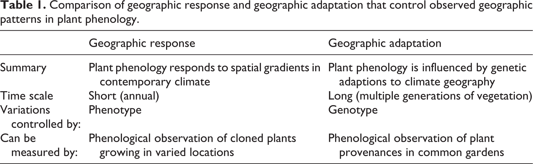
In particular, climatic controls of plant phenology operate at two drastically different temporal scales. One is instantaneous and accommodated by the phenotypic plasticity of plants, such as interannual weather effect on budburst timing. The other is long term, shaping plants’ genotypes through adaptation. The observed geography of plant phenology is hereby the result of both short-term and long-term climatic effects taking place over space at disparate temporal scales. Perhaps due to a limited integration of climatology and ecology (Pau et al., 2011), the two aspects of climatic influence have rarely been considered in tandem in identifying the causes of spatial variations in phenology. In fact, due to a ubiquitous emphasis on recent climate change, much attention has been given to short-term climate effects, while the genetic aspect of phenological variation is often neglected. As opposed to the directly measurable short-term climatic influences, long-term climate-shaped and genotype-based geographic variations are more difficult to quantify and separate from the observed patterns. Yet, for better understanding and modeling how the phenology of different species and populations of a species varies across space, it is critical to consider separately the phenotype-based geographic response and genotype-based geographic adaptation (Table 1). Here the geographic adaptation refers specifically to long-term climate-shaped genotypic differences over space, as being different from the geographic response that varies with year-to-year weather fluctuations.

Table 1.

Comparison of geographic response and geographic adaptation that control observed geographic patterns in plant phenology.

	Geographic response	Geographic adaptation
Summary	Plant phenology responds to spatial gradients in contemporary climate	Plant phenology is influenced by genetic adaptions to climate geography
Time scale	Short (annual)	Long (multiple generations of vegetation)
Variations controlled by:	Phenotype	Genotype
Can be measured by:	Phenological observation of cloned plants growing in varied locations	Phenological observation of plant provenances in common gardens

Clearly, genotype-based phenological variations are not completely determined by long-term environmental conditions via adaptation, but are also constrained by phylogeny (Davies et al., 2013; Davis et al., 2010; Pau et al., 2011; Willis et al., 2008). While more closely related species tend to leaf-out and flower at similar times, as phylogenetic conservatism indicates, they may do so because they are adapted to similar environments, implied by the notions of geographical conservatism and environmental filtering (Davies et al., 2013; Webb et al., 2002). Therefore, geographic adaptation may play a fundamental role in shaping genotype-based phenological variations over space, not only at the population and species levels, but also (at least in part) at the community and ecosystem levels.

Whereas the geographic response of plant phenology to climate gradients is relatively well-understood, the patterns of geographic adaptation remain unclear. Methodologically, geographic adaptation in plant phenology may be quantified using findings and principles of genecology, which studies adaptive differentiation of plant functional traits, often employing common gardens (Campbell and Sugano, 1979; Mátyás, 1996). But this body of research with particular respect to phenology is scattered, and has not been carefully examined in a way that would result in widely applicable geographic principles. On the other hand, the Bioclimatic Law offers foundational insight into the geography of plant phenology. But it relies on observed patterns only and falls short of accounting for the genetic diversity of plants, as noted previously. To move beyond the Bioclimatic Law, therefore, patterns controlled by geographic adaptation that are typical to many species need to be explicitly identified and clearly defined.

In this study, I synthesize literature from the rather loosely connected fields of phenology and genecology using common gardens, and incorporating findings from more recent cloned plant phenology research. The specific goal is to identify and define common geographic adaptation patterns and principles of plant phenology. This synthesis is focused on population level variations within respective species, but implications of the delineated patterns at the community and ecosystem levels are also discussed. Further, as the related knowledge base is mostly developed for temperature-driven plant phenology, especially for woody plants, I have focused the study on temperate trees. For plants growing in other environments, such as in drought-constrained climates where precipitation plays a more important role in triggering plant growth, additional research is required. Given the large amount of information on temperate trees and the typical seasonality they represent in the humid mid-latitude regions, the common patterns derived therein may serve as an initial yet fundamental step towards developing similar geographic principles in additional climates and biomes.

II Methods

Long-term climate-shaped genotypes interact with contemporary climate in complex ways to determine the timing of plant phenology. For many temperate plants, spring temperature drives phenology via two counter-balancing pathways (Chuine, 2000; Hunter and Lechowicz, 1992). First, a warming temperature is a prerequisite to resumed plant growth in spring, referred to as forcing or flushing temperatures. This is often measured with accumulated growing degree days or heat sum. Second, many temperate perennial plants only effectively respond to warming temperatures once winter dormancy (endodormancy) is released, which requires a substantial period of cold temperature accumulation (Coville, 1920; Rohde and Bhalerao, 2007; Schwartz and Hanes, 2010). This process is referred to as chilling or vernalization, through which plants are insured that the danger of frost has passed. The quantities of chilling and forcing, as well as the coordination mechanisms between the two, vary by species, and may be simulated in various ways (Chuine, 2000; Hanninen and Kramer, 2007). Further, photoperiod may interact with chilling and forcing to trigger spring budburst phenology. But its effect is limited to a few species and its role remains supplemental to the predominant effect of temperature (Basler and Körner, 2012; Caffarra et al., 2011b; Chuine et al., 2010). Autumn leaf phenology (growth secession and leaf senescence), on the other hand, though less studied than spring phenology, appears to be more routinely affected by shortening day length and cooling fall temperatures, with additional influences from environmental stresses (Fracheboud et al., 2009; Gallinat et al., 2015; Jeong and Medvigy, 2014; Xie et al., 2015). Therefore, on the one hand, plant phenology responds to year-to-year changes of these environmental factors (except for photoperiod, which is mostly static across years at a specific location). On the other hand, the geographic gradients of these climatic drivers entail a strong underlying geographic structure of plant phenology–climate (phenoclimatic) relationships that are embodied in different genotypes through long-term climatic adaptation.

Separating genotype-based geographic adaptation from geographic response with respect to their influence on the geographic patterns of phenology is possible through two methodological approaches (Figure 1). Both are based on the rationale that when one of the two variables is held as a constant, the observed variations are solely reflective of the other. First, by planting geographically different populations of the same species in a uniform environment, expressed phenological differences will be a function of genotypic variability only. This leads to an approach using common gardens, which permits the direct identification of adaptive variations within species in relation to different geographic origins. Field methodologies for common gardens (aka provenance tests), including the procedures for range-wide seed collection, the number of plantations, and the number of trees and replicates needed at each plantation, have been developed in forest genetics research (Wright, 1976). Many common gardens of tree species were established decades ago for silviculture and reforestation purposes (Morgenstern, 1996), and were later recognized to be valuable for examining intraspecific variations of plant growth in response to climate change (Mátyás, 1994, 1996). But most common garden studies were focused on juvenile plant survival and height growth, while phenology, as a supplemental trait related to growth, was observed only irregularly. Therefore, the phenological observation protocols used were often simple and lacking in detail. In spite of this limitation, essential adaptive variations of plant phenology are identifiable from common garden studies of many species.

Figure 1.

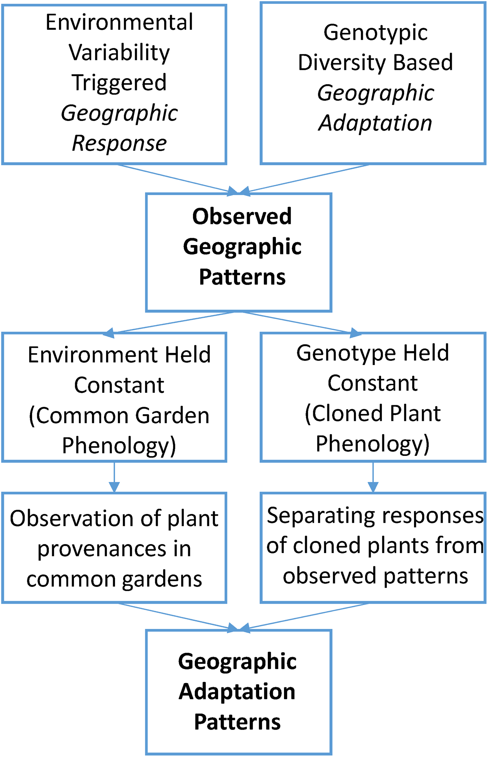
The methodological approaches to unveiling the geographic adaptation patterns in plant phenology.

An alternative approach holds the genetics constant while allowing the environment to vary, mainly through planting cloned plants (therefore, genetically identical) at different locations with diverse climatic conditions. The phenological response of cloned plants is uniformly a function of environmental differences. When compared to the phenology of common or naturally adapted plants, cloned plant phenology serves as a standard reference with respect to geographic response (cf. Table 1). Hence, to implement this approach two groups of individuals, viz., common plants and cloned plants, must be observed concurrently across a range of locations. The phenological difference between common plant and cloned plants reveals the degree of adaptation of the former. When these differences at various locations are plotted over an area of interest, the unveiled patterns would reflect variations contributed by geographic adaptation. The cloned plant approach is not as straightforward as common garden analysis and suffers a general lack of data. Although it complements common garden phenology by offering additional insights, cloned plant phenology research is still at its early stage of development (Liang and Schwartz, 2014). This synthesis is mostly based on ample literature on phenological observations in common gardens; limited findings from recent cloned plant phenology studies are discussed to provide a more complete view of the available methodological approaches.

III Adaptive patterns revealed in common gardens

The geographic adaptation variations observed in common gardens fall into three categories: (i) provenances from colder climates (e.g. related to higher latitudes or higher elevations) show earlier spring phenology than provenances from warmer climates (e.g. related to lower latitudes or lower elevations); (ii) conversely, provenances from colder climates have later spring phenology than those from warmer climates; and (iii) provenances from higher latitudes show earlier fall phenology than those from lower latitudes. The first case is referred to as being countergradient because the geographic gradient revealed in common gardens is opposite to that of populations growing in their source locations. And the latter two cases are cogradient given the same directions of the adaptation variations and the in situ observed geographic gradients. This terminology, adopted from evolutionary biology (Conover et al., 2009), helps illustrate and characterize the geographic adaptation patterns in phenology relative to the apparent geographic patterns (Figure 2). Below I provide examples of these patterns. While some representative cases are discussed in more detail, additional evidences are provided as citations.

Figure 2.

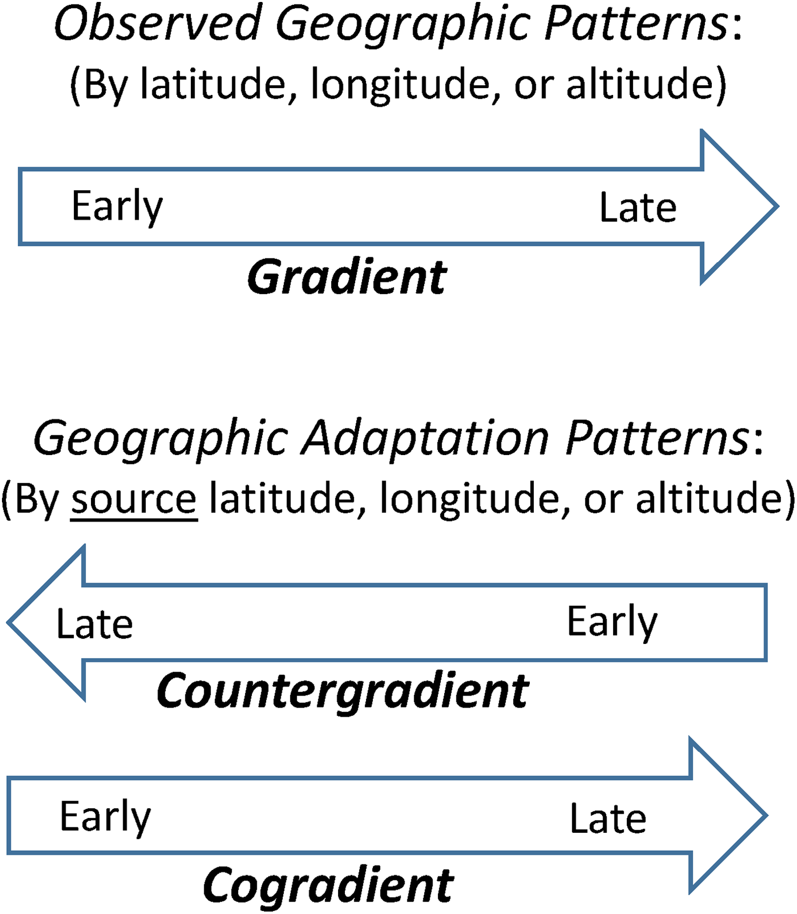
Concepts of countergradient and cogradient geographic adaptation patterns relative to gradient of observed patterns in plant phenology.

1 Countergradient pattern in spring phenology

A countergradient pattern in spring phenology involves bud break beginning with cold climate-adapted provenances and ending with warm climate-adapted provenances in a common garden. In a sugar maple (Acer saccharum Marsh.) common garden at Wooster, Ohio, northern provenances leafed-out sequentially earlier than southern provenances (Northern Hemisphere), showing a distinctive countergradient pattern (Kriebel, 1957). Further study at the same common garden using controlled chilling experiments showed that northern provenances required higher chilling than southern provenances for dormancy break, while under natural conditions at this common garden location in northern Ohio, trees from all sources obtained required chilling well before the end of the winter (Kriebel and Wang, 1962). Given that the chilling was not a constraint at this common garden, lower forcing requirements of the populations from colder climates led to earlier spring phenology, in turn manifesting a countergradient pattern.

This spatial trend is reversed (i.e. cogradient), however, for the same sugar maple progenies growing in a common garden in Gainesville, Florida, implying a delayed chilling fulfillment of the northern provenances at the warmer location (Kriebel and Wang, 1962). A similar experiment conducted at Gainesville, Florida, for red maple (Acer rubrum) also indicated that northern provenances of the species required higher chilling, while a provenance from the Everglades region of Florida showed no chilling requirement (Perry and Wu, 1960). Therefore, the expression of a countergradient pattern in spring phenology is related to a dominant influence of differential forcing requirements that are contingent upon an early fulfillment of chilling requirements for most provenances.

Additional common garden studies reporting a countergradient pattern similarly attributed this adaptation variation to differential forcing requirements of provenances. For instance, the spring phenology of balsam poplar (Populus balsamifera L.) was studied using data from two common gardens located, respectively, near the southern and northern edges of the species’ range in Canada and Alaska (Olson et al., 2013). The countergradient adaptive variation along latitude was more pronounced in the northern common garden than in the southern one, assumedly due to the fact that the chilling requirements of all provenances were fulfilled even earlier at the northern location, allowing for the effect of differential forcing to be manifested more thoroughly there.

Furthermore, the same countergradient pattern in Europe is sometimes more related to maritime-continental and topographic effects, leading to an adaptive geography predicted primarily by longitude and altitude. For example, leaf-out of European beech (Fagus sylvatica L.) occurred earlier in common gardens for provenances from inland Eastern Europe and higher elevations (Gömöry and Paule, 2011; Robson et al., 2013). Provenances adapted to warmer lowland and Atlantic drift-warmed coastal Western Europe appeared to require more forcing to trigger budburst, and thereby had delayed phenology in common gardens. In addition, the spring phenology of European beech is known to be sensitive to photoperiod (Heide, 1993; Vitasse and Basler, 2013), yet a lack of latitudinal gradient suggests that the influence of varied heat sum requirements is predominant in shaping its geographic adaptation pattern (Gömöry and Paule, 2011; Von Wuehlisch et al., 1995).

Examples of additional species that manifested a countergradient pattern in common gardens include silver birch (Betula pendula Roth) and downy birch (B. pubescens Ehrh.) (Myking and Heide, 1995); European ash (Fraxinus excelsior L.) (Pliura and Baliuckas, 2007); Norway spruce (Picea abies) (Eriksson et al., 1978); black spruce (P. mariana) (Johnsen et al., 1996); white spruce (P. glauca) and red spruce (P. rubens) (Blum, 1988); and Douglas fir (Pseudotsuga menziesii) (Campbell and Sugano, 1979).

2 Cogradient pattern in spring phenology

A cogradient pattern is observed as frequently as a countergradient pattern in the common garden studies of many tree species, which may have higher chilling requirements in general for dormancy release. In such cases, provenances adapted to colder climates leafed-out later due to delayed chilling fulfillment than those from warmer climates; and the effect of differential forcing requirements was apparently overridden. This is because if dormancy release is delayed from winter into spring, the start dates of forcing accumulation likely diverge for different provenances (with the cold climate-adapted ones being delayed further). In addition, the heat sum buildup occurs at a faster rate at a later date in spring due to higher effective temperatures, henceforth reducing the temporal differences of bud break caused by differential forcing requirements. These, in turn, lead to manifestation of the differences of dormancy break timing across provenances. In a study of red oak (Quercus rubra) in the southern Appalachians, provenances from different elevations were grown in common gardens located across an altitudinal range similar to that of the acorn sources (McGee, 1974). In all common gardens, bud break occurred sequentially from low-altitude provenances to high-altitude provenances, displaying a consistent cogradient trend. This phenomenon suggests a strong chilling-controlled spring phenology of the species.

In another case, leaf unfolding and seed germination of sessile oak (Quercus petraea) were also found to be earlier for southern provenances than northern provenances in common gardens (Alberto et al., 2011; Deans and Harvey, 1995; Ducousso et al., 1996). These common gardens of sessile oak were located in either low-lying French cities near the Atlantic coast (Alberto et al., 2011; Ducousso et al., 1996) or at Edinburgh, Scotland, which has a similarly temperate climate (Deans and Harvey, 1995). The locations of these common gardens optimized the chance of hindered chilling fulfillment for cold climate-adapted provenances. Although the role of chilling is not explicitly mentioned in the above studies, the adaption of sessile oak to higher risks of frost damage through delayed spring phenology in colder climates is acknowledged. A lack of understanding of chilling as a determinant of budburst timing variation, however, might have led to unjustified assumptions that low-latitude provenances require less heat sum for sessile oak (Deans and Harvey, 1995; Liepe, 1993) and other species such as white ash (Fraxinus americana L.) (Marchin, 2010).

Additional studies that documented a cogradient pattern of spring phenology include black cherry (Prunus serotina Ehrh.) (Barnett and Farmer, 1980; Cech and Carter, 1979); black walnut (Juglans nigra L.) (Bey et al., 1971); silver maple (Acer saccharinum L.) (Ashby et al., 1992); field elm (Ulmus minor) (Ghelardini et al., 2006); paper birch (Betula papyrifera Marsh.) (Hawkins and Dhar, 2012); and maritime pine (Pinus pinaster) (Desprezloustau and Dupuis, 1994). This partial list may imply generally higher chilling requirements of the species. But caution needs to be exercised to avoid overgeneralization, given additional influences of the climates and interannual weather fluctuations at respective common garden locations. Given the importance of understanding this context, below I elaborate in more detail the factors that control the expression of alternative geographic adaptation patterns in spring phenology.

3 Factors controlling the expression of adaptation patterns in spring phenology

The interactions of different environmental factors that trigger spring phenology are complex and difficult to entangle. The usually very large interannual variations of budburst phenology suggest that temperature’s role is predominant over photoperiod, given the stationarity of the latter. However, the temperature effect alone, comprising two counteracting mechanisms (i.e. forcing and chilling), is far from being straightforward, but may lead to varied and sometimes ambiguous expressions of geographic adaptation patterns. Detailed phenological observations with concurrent meteorological measurements in a white ash common garden (located in the species’ central range) suggested that while a strong chilling-controlled cogradient pattern may be shown in a year with a mild to normal prior winter, an unusually cold winter can lead to manifestation of a countergradient pattern instead in the same common garden (Liang, 2015).

Therefore, the expression of a countergradient or a cogradient pattern in spring phenology in a specific common garden likely depends on: (i) the respective levels of chilling and forcing that are required by a given species in general; (ii) the direction and magnitude of temperature change simulated by seed transfer from populations’ source locations to the location of the common garden; and (iii) the winter and spring temperature regimes during the years of observation at the common garden location. The first two factors have been discussed sufficiently. To further expand on the role of interannual weather change, the use of alternative scenarios can provide some insights. Specifically, in a cold winter-cool spring scenario, when chilling demand is unanimously met for all provenances in winter and forcing is built up gradually in spring, a marked, differential forcing-induced countergradient pattern is likely expressed. On the other hand, in a mild winter-warm spring scenario, when chilling fulfillment is significantly delayed and dormancy release sufficiently restrained for all provenances, and with fast subsequent thermal accumulation, a distinct differential chilling-controlled cogradient pattern would be manifested. Furthermore, in a mild winter-cold spring scenario, budburst of cold climate-adapted provenances is likely delayed due to insufficient winter chilling while the provenances from warm climate are similarly delayed hereafter by a lack of spring forcing, possibly leading to indefinite patterns. Finally, in a cold winter-warm spring scenario, earliest budburst is expected for all provenances because both chilling and forcing requirements are optimally satisfied. This scenario may lead to a weak countergradient pattern, given an early fulfillment of chilling requirements and a subsequent faster (compared to the cold winter-cool spring scenario) accumulation of forcing temperatures.

4 Cogradient pattern in autumn phenology

In comparison to spring phenology, autumn phenology of temperate plants is predicted by a less complex set of routine environmental cues, primarily declining day length and cooling temperature (Jeong and Medvigy, 2014; Yu et al., 2016). Perhaps contrary to the understanding that fall phenology is more complex than spring phenology, the environmental drivers of fall phenology are simpler in the sense that a counteracting temperature effect (i.e. chilling vs. forcing) is absent and the less variable day length plays a more significant role. Photoperiod is known to govern growth secession and dormancy induction of many trees (Rohde and Bhalerao, 2007). Although additional environmental factors such as heat, frost, wind, and especially drought may also trigger early leaf senescence in temperate forests (Leuzinger et al., 2005; Munn-Bosch and Alegre, 2004; Panchen et al., 2015; Xie et al., 2015), they operate more as stress factors rather than routine drivers under normal weather conditions. It is difficult, therefore, to tease out the impact of these factors on the geographical adaptation patterns of autumn phenology in temperate regions.

Notably, a nearly unanimous cogradient pattern of autumn phenology is found in common gardens in spite of disparate expressions of either a cogradient or a countergradient pattern in spring phenology of the same species (examples follow). As in situ fall leaf coloration or leaf fall occurs earlier in the north and later in the south (Northern Hemisphere), a cogradient pattern in fall phenology timing indicates an adaptation gradient that matches this observed geographic transition, which is the opposite to that of spring phenology. As evidenced by limited common garden studies using detailed phenological observation protocols, the cogradient pattern in fall phenology appears to be highly consistent across years and features smoother spatial transitions than that of spring phenology (Liang, 2015). Such a cogradient pattern can only be attributed to a latitudinal gradient of photoperiod rather than temperature. Otherwise, assuming that northern provenances are more tolerant to cooling fall temperatures, they would retain leaves longer than southern provenances. This would lead to a hypothesized countergradient pattern, which is contrary to the observation. Indeed, the high-latitude provenances are likely adapted to higher critical photoperiod (longer day length) thresholds (Rohde and Bhalerao, 2007) and, therefore, have earlier leaf senescence than the low-latitude provenances in common gardens. This is supported by the fact that photoperiod change plays a leading role in regulating the timing of fall phenology (Allona et al., 2008; Way, 2011). Such a mechanism favors northern populations by more effectively minimzing the risks of frost damage at higher latitudes. However, this does not rule out the role of temperature in the context of interannual variability. For plants growing at their original latitudes, while photoperiod sets up the fundamental limits to the timing of leaf senescence, temperature fluctuations (along with environmental stresses) do further influence the process of triggering plant growth secession, thereby causing interannual variations.

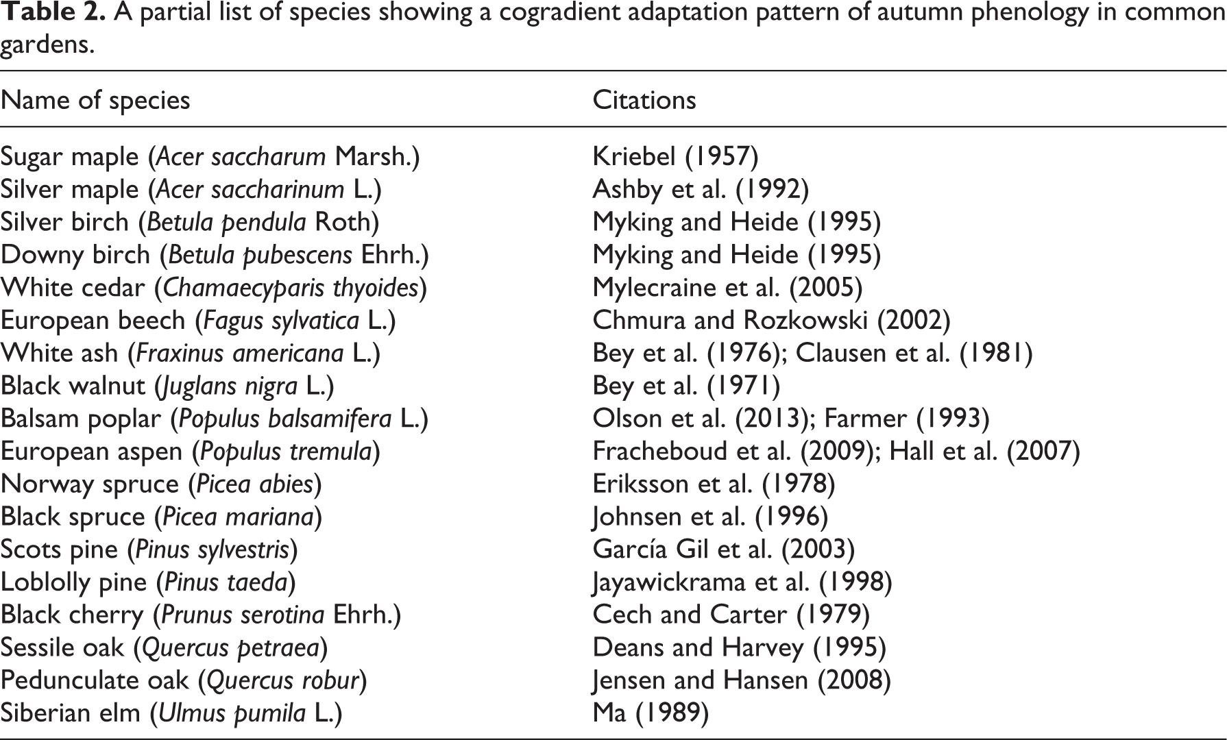
For all species surveyed, akin to an earlier review of North American trees (Nienstaedt, 1974), leaf fall, and leaf coloration almost always start from high-latitude populations, and end with low-latitude populations in common gardens. Such a cogradient pattern in autumn phenology is observed for many tree species provided in the partial list in Table 2. The large number of works on a cogradient pattern in fall phenology bears eloquent testimony to the existence of a strong photoperiod-sensitive adaptation mechanism. A diagram summarizing geographic adaptation patterns of both spring and fall phenology along a latitudinal gradient is provided in Figure 3.

Figure 3.

Geographic adaptation patterns in temperate plant phenology along a latitudinal gradient in the Northern Hemisphere for both spring and fall seasons. The dash-line shape indicates a hypothesized but unobserved pattern.

Table 2.

A partial list of species showing a cogradient adaptation pattern of autumn phenology in common gardens.

Name of species	Citations
Sugar maple (Acer saccharum Marsh.)	Kriebel (1957)
Silver maple (Acer saccharinum L.)	Ashby et al. (1992)
Silver birch (Betula pendula Roth)	Myking and Heide (1995)
Downy birch (Betula pubescens Ehrh.)	Myking and Heide (1995)
White cedar (Chamaecyparis thyoides)	Mylecraine et al. (2005)
European beech (Fagus sylvatica L.)	Chmura and Rozkowski (2002)
White ash (Fraxinus americana L.)	Bey et al. (1976); Clausen et al. (1981)
Black walnut (Juglans nigra L.)	Bey et al. (1971)
Balsam poplar (Populus balsamifera L.)	Olson et al. (2013); Farmer (1993)
European aspen (Populus tremula)	Fracheboud et al. (2009); Hall et al. (2007)
Norway spruce (Picea abies)	Eriksson et al. (1978)
Black spruce (Picea mariana)	Johnsen et al. (1996)
Scots pine (Pinus sylvestris)	García Gil et al. (2003)
Loblolly pine (Pinus taeda)	Jayawickrama et al. (1998)
Black cherry (Prunus serotina Ehrh.)	Cech and Carter (1979)
Sessile oak (Quercus petraea)	Deans and Harvey (1995)
Pedunculate oak (Quercus robur)	Jensen and Hansen (2008)
Siberian elm (Ulmus pumila L.)	Ma (1989)

IV Adaptation patterns revealed using cloned plant phenology

In addition to the common garden approach, geographic adaptation patterns in phenology can be derived by removing cloned plants-based geographic response variability from observed patterns (cf. Table 1, Figure 1). The spatial variation in the amount of difference between the concurrently observed common and cloned plants (e.g. departure of budburst dates) can be used to infer geographic patterns controlled by adaptive differentiation. Studies employing this approach are very rare, with only one published study to date (Liang and Schwartz, 2014). The dataset used in this study is for first leaf and first bloom of cloned lilac (Syringa x chinensis ‘Red Rothomagensis’), which has been observed within certain regional networks in the US since the 1950s (Schwartz et al., 2012). This effort has now been continued by the USA-National Phenology Network (USA-NPN) since 2009. The USA-NPN also collects phenological data of many other common plant species and included an additional cloned plant, cloned dogwood (Cornus florida ‘Appalachian Spring’). These data will undoubtedly increase the opportunities of using the cloned plant approach to investigate plant geographic adaptation patterns in the future.

Ideally, cloned plants should be compared with common plants of the same species, but such data are not currently available. A drawback of comparing cloned plants with common plants of a different species is that the absolute difference between the phenological timing of the two does not carry direct biophysical meaning. But given that cloned plant phenology is not influenced by genetic variations, the geographic gradients (not absolute dates) of phenology of different clones would reflect similar bioclimatic gradients. Therefore, the spatial gradient (not the absolute values) of the differences between the phenologies of cloned and common plants of different species can still reflect spatial adaption differentiation of the latter, hence indirectly revealing its geographic adaptation pattern. Indeed, the first leaf and first bloom dates of cloned lilac showed significantly steeper latitudinal gradients than that of common plants in the temperate eastern US (Liang and Schwartz, 2014). This finding implies that cold climate-originated natural populations are adapted to lower thermal forcing requirements, hence with relatively (vs. absolutely) earlier phenology with respect to cloned plants at the same locations, and vice versa for natural populations growing in warmer climates. This climatic adaptation leads to dampened latitudinal gradients for common plant phenology than that of cloned plant phenology, which reflects geographic response only. This relationship concurs with that of a countergradient pattern in common gardens due to differential forcing. The role of chilling is not obvious in cloned plant phenology studies given that all observations were taken in situ and chilling requirements were likely fulfilled very early in most occasions.

V Implications, applications, and future directions

1 Climate change impact on spring and fall phenology over space

The forcing-based countergradient and chilling-based cogradient patterns in spring phenology reveal two interwoven pathways of climate change impact on temperate trees. The countergradient pattern suggests that, in general, the same amount of spring temperature increase may trigger larger earlier shifts in spring phenology of cold climate-adapted plants than warm climate-adapted plants, contingent upon an early chilling fulfillment. A study using data from the USA-NPN predicted that the mean budburst date will likely advance more in the north than the south in the Northern Hemisphere under projected future climate scenarios (Jeong et al., 2013). On the other hand, contrary to a popular understanding of earlier phenology triggered by climatic warming, insufficient chilling may instead delay spring phenology of many species (Cook et al., 2012). However, current and anticipated magnitudes of climate warming (e.g. <2°C) are far less than climate change simulated by common garden experiments (e.g. 10–20°C, as in a space-for-time substitution scenario), making chilling shortage less likely to occur for locally grown plants on a regular basis. This generalization does not exclude cases when chilling fulfillments of certain species or vegetation in particular regions are hampered by anomalously warmer winter weather (Yu et al., 2010). Indeed, over the past century, climate change in the US, for example, has shown variability both seasonally and across regions, with temperature increase being more prevalent in the north and during the winter season (Capparelli et al., 2013; Menne et al., 2009). In addition, both observational and predictive studies have suggested that the spring phenology of northern forests is more likely affected by a chilling deficit during years with mild winters (Kaduk and Los, 2011; Liang and Zhang, 2016). Therefore, while the forcing-based countergradient mechanism is most applicable under the current climate regime, at least for specific regions and species that have relatively higher chilling requirements, it is necessary to consider the influence of an underlying chilling-based cogradient mechanism to avoid overestimating warming-induced spring phenological advances. In either case, the spring phenology of plants in warmer parts of the temperate climate may be less affected by global warming given their generally greater demands for heat energy as well as lower requirements for chilling.

Fall phenology, however, is affected differently across space by climate change given its unique environmental cues (Way, 2011; Xie et al., 2015). Although in addition to photoperiod and temperature, other factors, especially water stress, may trigger early leaf senescence (Leuzinger et al., 2005), precipitation is not a routine driver of fall phenology in temperate forests (Dragoni and Rahman, 2012; Liu et al., 2016). Hence, while environmental stresses may cause changes in the fall phenology of temperate trees at local to regional scales in specific years, the majority of the spatial variations in fall phenology is still governed by photoperiod and temperature. In fact, for the humid temperate forests in the eastern US and Japan, amid the general delaying effect of climate warming on the end of the growing season, northern tree populations and vegetation tend to be less sensitive (with smaller interannual variations) to temperature increase (reduced summer-to-fall chilling) than those in the south (Doi and Takahashi, 2008; Dragoni and Rahman, 2012). This latitudinal trend of climate change impact is opposite to that of spring phenology, and has important implications about the relative roles of photoperiod vs. temperature in regulating the timing of fall phenology. In the light of a consistent cogradient adaptation pattern in autumn phenology for most temperate tree species, this latitudinal difference in temperature responsiveness suggests that photoperiod gradient regulates the timing of growth cessation and leaf senescence predominantly. This is supported by the fact that in high-latitude regions with greater early fall frost risks, more rigid photoperiod control vs. temperature response appears to be a favorable adaptive trait. Whereas in the south, plants may be less constrained by photoperiod and, therefore, are more flexible in responding to temperature fluctuations, perhaps allowing some extra extension of the growing seasons. The larger and faster photoperiod change at the higher latitudes may also contribute to forming a stronger photoperiod cue in driving fall phenology in colder regions. There are, however, exceptions to this general relationship for certain species (Tanino et al., 2010). Nonetheless, given the leading role of photoperiod in regulating fall phenology according to the known physiology of many species (Allona et al., 2008; Rohde and Bhalerao, 2007; Way, 2011), the impact of climate warming on temperate trees in the autumn season is likely more constrained, and is probably more so towards higher latitudes.

2 Building spatially explicit phenological models

In the absence of clearly defined geographic adaptation patterns, predicting phenological variations induced by spatial heterogeneity in plants is hardly possible. Delineation of intrinsic adaptation geography in phenology, therefore, comprises an essential step towards building phenological models that are capable of predicting spatially explicit phenological responses to climate change. The existing phenological models, which are developed primarily for spring phenophases (leaf-out or flowering) of temperate woody species, have commonly focused on the instantaneous climatic effects on a few specific plant populations (Chuine et al., 2013; Hanninen and Kramer, 2007). To achieve a broad geographic coverage, one can utilize cloned plant phenology to produce standard responses to meteorological variables at the continental scale, as represented by the widely used spring indices models (Schwartz, 1997; Schwartz et al., 2006, 2013). Alternatively, more physiologically specific models (e.g. unified models) may be fitted for discrete natural populations of selected species across various locations independently (Chuine, 2000; Xu and Chen, 2013). The latter approach using multiple spatially independent models partly addresses the need to enable spatially explicit prediction capability, but is technically inefficient and lacks the power to extend the predictions to where data and models are not available. On the other hand, cloned plants-based models are advantageous in a sense that they offer continuous spatial coverage (limited only by the availability of weather data). Yet in both cases, an underlying spatial structure, as can be furnished by the geographic adaptation patterns defined in this study, is missing.

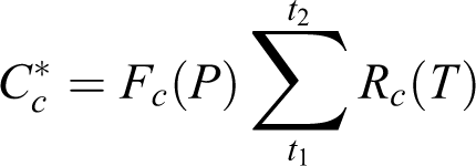
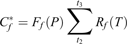
Moving forward from these previous developments, a way to construct spatially explicit phenological models, therefore, lies in combining the strengths of the above two approaches through incorporating the geographic adaptation patterns. The goal is to produce a single model over a region of interest for a given species and event (e.g. spring leaf-out) that is driven by both climatic and genotypic variables. Traditional models use fixed parameters fitted for specific populations. In a spatially explicit model, however, the parameters are geographically dependent. To better illustrate this idea, I offer the following conceptual model, using a simple 2-phase (chilling and forcing) sequential structure for spring leaf-out phenology as an example. A traditional approach is embodied in the following equations:

Phase 1

C_{c} = \sum_{t_{1}}^{t_{2}} R_{c} (T)

where C_c is the critical amount of chilling needed for breaking endodormancy (deep dormancy maintained internally by plants; Rohde and Bhalerao, 2007); t₁ is the time when chilling starts to accumulate (may be arbitrarily set as an constant, e.g. October 1 of prior year), and t₂ is when chilling requirement is met and endodormancy is broken; R_c is the rate of chilling, which is calculated from hourly or daily temperatures (T), according to specific base temperatures and response functions (Chuine et al., 2013).

Phase 2

C_{f} = \sum_{t_{2}}^{t_{3}} R_{f} (T)

where C_f is the critical amount of forcing needed after endodormancy break to complete ecodormancy (shallow dormancy maintained by environmental conditions) and trigger leaf budburst; t₂ is the time of endodormancy break, and t₃ is the date of budburst; R_f is the rate of forcing, which is similarly calculated from hourly or daily temperatures (T), according to specific base temperatures and response functions, in the simplest scenario, as growing degree days (Chuine et al., 2013).

In a spatially explicit model, the chilling and forcing requirements will vary across populations/locations, as can be predicted by specifically defined geographic adaptation patterns for a particular species, rather than independently for each population/location. Therefore, this additional level of variability needs to be incorporated into the previous equations as embedded functions, potentially in the following forms:

Phase 1

C_{c}^{*} = F_{c} (P) \sum_{t_{1}}^{t_{2}} R_{c} (T)

Phase 2

C_{f}^{*} = F_{f} (P) \sum_{t_{2}}^{t_{3}} R_{f} (T)

where $C_{c}^{*}$ and $C_{f}^{*}$ are average critical chilling and forcing requirements of a species, respectively; F_c(P) and F_f (P) are functions predicted by varied populations (P) to adjust for differential chilling and forcing requirements across space. Here the critical chilling and forcing requirements are kept as constants and specific to a species, while the population level variability is characterized using the embedded functions. This treatment allows the species level and population level variabilities to be separately represented in the models. The population functions, viz., F_c(P) and F_f (P), are based on the geographic adaptation patterns specifically delineated for that species, and, in turn, may be predicted by geographic coordinates (e.g. latitude, longitude, and elevation), according to the cogradient (for phase 1) and countergradient (for phase 2) relationships, respectively. Both linear and nonlinear functions can be used for defining specific F_c(P) and F_f (P) for a given species, but the general trends (i.e. cogradient and countergradient) should remain consistent. This conceptual model structure allows a single model to be built for a species over a broad region, ideally covering its entire distribution range, despite the fact that the actual presence or realized niche of the species may have gaps within its range.

Given the diversity of phenoclimatic mechanisms of varied species, the spatially explicit phenological models may take on alternative forms with more or less complexity. For species that do not show obvious chilling requirements (likely satisfied early in winter), model structures may be simplified to include the forcing component only (Schwartz et al., 2013). Or, for species with more intricate environmental cues and physiological processes, more involved parameterization and model structure formulation are required (for a review of the different types of models, see Chuine et al., 2013). These cues and processes involve species with strong photoperiod responsiveness (Basler and Körner, 2012), differential dormancy induction dates (Caffarra et al., 2011b), parallel and alternating relationships between chilling and forcing (Hanninen and Kramer, 2007; Murray et al., 1989), and sensitivities to synoptic weather events (Schwartz and Marotz, 1988). Customized models need to be fitted to data for respective species according to the best known phenoclimatic relationships. Clearly, implementing these ideas and models requires substantial future work, not only because the detailed geographic adaptation patterns for particular species are yet to be accurately quantified, but also because our knowledge about the exact phenoclimatic mechanisms of plants remains scarce. At the current stage of developing spatially explicit phenological models, the generalized geographic adaptation patterns serve to substantiate the theoretical feasibility (i.e. proof-of-concept) and provide a geographic framework for more detailed works in the future.

In addition, modeling of fall phenology, though often neglected and perceived to be more complex than spring phenology (Gallinat et al., 2015), may turn out to be rather straightforward in a geographic context, given its highly consistent cogradient adaptation pattern. Improved fall phenology modeling is certainly needed for better constraining the growing season length. In addition, it may be necessary for accurately predicting spring phenology of certain species, given the necessity to account for different dormancy induction dates (Caffarra et al., 2011a). Apparently, winter does not always reset the calendar of perennial woody plants with respect to the cycles of growing and non-growing seasons. Unless there is a sufficient temporal interval between endodormancy break and the starting date of thermal accumulation, as in the case when chilling requirement is fulfilled early in winter before temperature rises above a critical threshold to allow for effective forcing, the timing of fall phenology in the previous year may well be a part of the equation for predicting the timing of spring phenology in the following year. A similar carry-over effect is reported for the spring-to-fall period (i.e. throughout the growing season) as well (Keenan and Richardson, 2015). Hence, fall phenology modeling should be given more attention and ideally implemented in tandem with spring phenology. Spatial structures akin to the conceptual model provided for spring phenology may be used, with photoperiod (incorporated according to the cogradient adaption pattern) and temperature as primary predictor variables. Overall, phenology as a precursory sign of more profound changes in the biosphere (details follow) should be more fully used in prognostic applications. Knowing that geographic diversities of phenological timing are not random and discrete over space, but are governed by traceable patterns predefined by long-term environmental gradients, allows us to enable spatially explicit capability for phenological forecasting, thus to bring this effort to a new level.

3 Tracking ecological processes and species distribution

The ecological consequences of phenological change in plant species are far reaching and occur in geographically explicit contexts. As a crucial component of ecological processes and functions, plant phenology regulates carbon exchange and primary productivity (Richardson et al., 2010), synchronizes or desynchronizes trophic interactions (Rafferty et al., 2015), and limits species distributions (Chuine, 2010; Chuine and Beaubien, 2001). In the face of climate change, the capacity for temporal shifts in organismal life cycles via phenotypic plasticity is not unlimited. Surpassing the limits of plastic response through timing changes of growth and reproductive events will ultimately affect the survival and development of organisms. Consequently, local extinction and/or microevolution of certain species are likely to follow, leading to species range shift and/or community reconfiguration (Chuine, 2010; Gienapp et al., 2008). The temporal adjustment of plants via phenotypic plasticity is thus intrinsically linked to the spatial adjustment of species in response to climate change (Chuine, 2010; Chuine and Beaubien, 2001). Such sequential change demonstrates that changes to a particular ecosystem in the temporal domain via phenological shift are precursory and early-warning signs of further and more drastic changes in spatial and genetic domains. Especially for sessile plants that cannot migrate as individuals and whose dispersal abilities are limited, the impacts of phenological change on community and ecosystem functions may be substantial. In addition, different rates of phenological change in related species that exist in predator–prey, herbivore–host, and mutualism relationships will lead to trophic mismatch and asynchrony in their life processes (Kudo and Ida, 2013; McKinney et al., 2012; Thackeray et al., 2010). Hence, drawing a clear picture of the intrinsic geographic adaptation patterns in plant phenology and building spatial models accordingly can potentially help determine the time and location of the subsequent transitions from phenotypic plasticity-supported timing shifts to more fundamental changes in genetics, distribution, and interaction of species.

In particular, the distribution of species is affected by phenology given that the survival, growth, and reproduction, hence, the fitness of plants, is closely tied to their ability to successfully fulfill the annual cycle of growth in a given climate (Chuine, 2010; Chuine and Beaubien, 2001). Previous studies hypothesized that at the northern limit, the fitness of populations of a temperate species is limited by frost damage and short growing seasons, while at the southern limit the restrictions are set by unfulfilled chilling requirements. Certain models have used phenology as a predictor of species distribution in line with these hypotheses (Morin et al., 2007, 2008). But these hypotheses and associated models have not taken into account the varied climatic requirements of plant populations within a species’ range, as reflected in the identified geographic adaptation patterns. For instance, southern populations of certain species may have lower chilling requirements with the result that the impact of warming on spring phenology is likely smaller compared to northern populations under the same magnitude of temperature change, as pointed out previously. Hence, there is a need to improve these phenology-dependent species distribution models by supplying explicit spatial parameters that represent the within-range genotypic variability of species. As a further step beyond developing spatially explicit phenological models, range-wide predictions of phenological change based on specific geographic adaptation patterns of a given species can be used as a critical input to improve the performance of species distribution models. In addition, integrating spatial models of phenology and species distribution may facilitate simulation and evaluation of the spatial variability of species interactions (Liang and Fei, 2014; Rafferty et al., 2013). In the long run, this will potentially bridge the temporal and spatial aspects of biospheric responses to climate change in a prognostic modeling framework. Such an integrated system with temporal shifts being precursory and range shifts being consequential components, for instance, may provide a more comprehensive and cohesive approach to the ecological impacts of climate change.

4 Monitoring inherent vegetation changes and biological invasions

In addition, given that the adaptive geography of phenology provides an intrinsic view of genotypic characteristics of plants that are free from instantaneous environmental influences (e.g. year-to-year weather fluctuations), it can be utilized to track inherent changes in vegetated landscapes. Remotely sensed land surface phenology has been employed for forest health monitoring using anomalous phenological departures as signals of disturbance (Hargrove et al., 2009), and mapping ecosystems based on diversified timing behaviors of seasonal land covers (Loveland et al., 1995). The current synthesis focuses on adaptation patterns at the population and species levels. But given that phylogenetic conservatism is expressed in the species’ geographical co-occurrence patterns (Davies et al., 2013), especially through environmental filtering (Webb et al., 2002), the geographic adaptation patterns in phenology are likely applicable at the community and ecosystem levels as well (Kaduk and Los, 2011). A recent study estimated the underlying climate adaptation patterns of temperate vegetation at the ecosystem level, using land surface phenology standardized by predictions from cloned plants-based models (Liang et al., 2016). These ecosystem-level geographic adaptation patterns in phenology, once periodically derived on a regular basis, may be used to more accurately detect non-weather-related vegetation changes, such as those caused by succession and disturbances.

The geographic adaptation patterns are applicable mostly to native and naturalized plants and communities. In a world with its biota being increasingly dispersed and rearranged over space, the phenological patterns determined at the ecosystem level are subject to modifications at specific locations. For example, many exotic and/or invasive plant species (mostly understory) often take advantage of vacant phenological/temporal niches in relation to canopy trees to increase their fitness, such as via prolonged growing seasons (Fridley, 2012; Polgar et al., 2014; Smith and Reynolds, 2015; Wolkovich and Cleland, 2011). Agriculture further adds to the uncertainties of applying the derived patterns to specific regions because crop composition and planting time are modified by human management, thereby missing a large part of the adaptive variation from natural vegetation. Hence, both exotic species and land cover/land use are expected to complicate the geographic adaptation patterns manifested, especially when looking at specific locations. On the other hand, however, departures from the predicted geographic adaption patterns can be used as a tool to gauge the degree and extent of human modification to natural landscapes. This idea echoes back to the rationale of using geographic adaptation patterns to detect inherent vegetation changes, as elaborated previously.

Furthermore, knowledge of adaptive geography in phenology can be potentially used to track biological invasions in novel ways. In particular, matching adaptive phenological traits of an introduced population with that of populations in the species’ native range can help reveal the geographic origin of the introduced population. This is a reversed application of the concept of common garden, in which the source locations of populations are known. Practically, this can be done by comparing the difference between phenologies of exotic and native populations of the species with that of a cloned plant, if they are observed in the field. Information from the exotic species alone (i.e. without a clonal reference) cannot achieve this because phenological timing varies across environments via phenotypic plasticity. The cloned plant phenology approach is, therefore, needed in this circumstance to identify the degrees of adaption for both exotic and native populations. But if resources allow, putting the introduced and native populations into a common garden or controlled experiment setting may achieve the same (probably better) result. Conceptually, this comparative phenology approach may also be used to discover invasive populations at various stages of naturalization/adaptation, hence to retrospect histories and pathways of specific introduction/invasion scenarios. Given that phenology is one of the most conspicuous functional traits of plants, knowing the linkages between its variations and the underlying genotypic differences is useful for quickly identifying intrinsic relationships among plant populations and species across geographical space.

5 Future directions

Continued and improved common garden phenology observation and analysis are still needed to determine detailed adaptation patterns for selected species. Many of the phenological observations recorded in literature were for juvenile plants during the initial years after the plantations were established. Young plants and adult trees, however, have shown different spring phenology due to ontogenetic changes, with the former generally leafing out earlier (Vitasse, 2013). This age effect on phenological timing matters for evaluating climate change impact on trees in growth chamber experiments using seedlings. But with respect to detecting the geographic adaptation patterns, the spatial relationships found for juvenile plants should still hold, because the provenances were observed at the same time and same ontogenetic stages. The consideration of ontogenetic differences of seedlings vs. trees, however, is needed for improving future phenological observations in common gardens. Especially, instead of establishing new common gardens, phenological observations in historically established ones (hence, with matured trees) are preferred to better match observations to responses of canopy trees in natural stands. Ideally, more dedicated phenological observation protocols with concurrent onsite environmental measurements should accompany this effort (Liang, 2015). An awareness of the value of historical common gardens for climate change impact and adaptation research has been increasing (Alfaro et al., 2014; Leites et al., 2012; Mátyás, 1996). However, many previously established (but later abandoned or not actively used) provenance test sites are yet to be discovered and properly maintained to allow access and data collection.

Further, to directly measure the phenoclimatic requirements of different plant populations, thus to more accurately specify the geographic adaptation patterns of certain species, controlled experiments may offer the best odds. To date, determination of chilling and forcing requirements of particular species have relied on indirect estimation using statistical methods (Ashcroft et al., 1977; Luedeling et al., 2013; Pitacco et al., 1992; Schwartz, 1997). Certain models are more constrained by known physiological processes, but still require statistical fitting (Chuine, 2000; Hanninen and Kramer, 2007). Certainly, the experimental approach used together with common gardens is labor- and resource- intensive, but it could yield significant information for precisely parameterizing spatially explicit phenological models. This effort is challenging and moves towards reaching the “holy grail” of linking phenological variations across physiological and climatological scales (Pau et al., 2011). Given the age effect noted above, cuttings from mature trees (vs. seedlings) are preferred in such experiments (Vitasse and Basler, 2014).

Along the lines of cloned plant phenology, further work is needed to include additional species and develop new methods to extract geographic adaptation patterns. This work is becoming more promising with the growing datasets from the Nature’s Notebook program of the USA-NPN, which covers both cloned indicator plants and naturally adapted species (Denny et al., 2014; Liang and Schwartz, 2014; Schwartz et al., 2012). In spite of the limitations in relation to measurement accuracy and precision that typically come with crowd-sourced data (remediable with effective quality control procedures), as well as mixed signals from horticultural plants, the USA-NPN dataset offers broad geographic coverage and a rich variety of species, and, therefore, provides unique opportunities for developing and testing spatially explicit phenological models.

Moreover, expanding the principles of geographic adaptation to areas beyond the temperate regions in relation to spatial gradients of additional environmental factors, such as precipitation, should not be ruled out in future studies. While more detailed work is still needed to further our understanding of the patterns in temperate plant phenology, and there is generally a lack of similar literature in support of a synthesis as such in other geographic domains, information from satellite remote sensing (along with available ground-based observation) may help initially explore ecosystem-level geographic adaptation patterns in additional biomes.

Finally, the dynamic interactions between life and climate, over both time and space, and across multiple spatial and ecological scales, converge at and are highlighted by the study of the geography of plant phenology. Continued exploration of the intrinsic geographic patterns in plant phenology, on fronts of both theoretical development and practical applications, will undoubtedly expand our scope of knowledge along this line of research. Beyond the Bioclimatic Law, which summarized the apparent geographic pattern in plant phenology, the current work proposes a further step to establish the underlying geographic principles, as embodied in the derived geographic adaptation patterns.

VI Conclusions

Phenology represents the biological aspect of seasonality, and its changes and geography vividly reflect the importance of unifying temporal processes and spatial patterns. This article synthesized knowledge concerning the intrinsic genotype-based variations of temperate plant phenology and identified corresponding geographic adaptation patterns. These patterns are characterized as being either countergradient or cogradient in common gardens relative to the in-situ observed geographic gradients in plant phenology. Both a cogradient pattern and a countergradient pattern are inherent to the spring phenology of many temperate tree species. The former is caused by different chilling requirements of populations, and the latter by different forcing requirements, either of which can be more dominant for particular species and/or under specific climatic conditions. Fall phenology of most tree species demonstrates a consistent cogradient pattern that is tied to a latitudinal photoperiod gradient.

The current work facilitates linking the temporal domain of plant activities more explicitly to its spatial domain, and provides meaningful guidance to important research topics in relation to bioclimatic interactions of organisms. Practically, the defined geographic adaptation patterns are useful for building spatial models that can track geographically distinct phenological responses to climate change, and to potentially improve the accuracy of predicting species’ range shift, among other associated ecological changes. Additionally, adaptive geography in phenology offers novel tools for monitoring inherent vegetation changes and biological invasions. More work is still needed to specifically quantify the geographic adaptation patterns for selected species, mainly through improved common garden observations and controlled experiments, and furtherance of cloned plant phenology research. Overall, a better understanding of the adaptive geography of plant phenology lays the foundation for tracking spatially variable interactions between climate and life. In the face of the environmental challenges in relation to climate–life relationships, phenology will play a more effective role with better-developed geographic theories and models. This synthesis serves as an initial step to make the way for accomplishing these tasks, and hopefully will contribute to furnishing a stronger and more clearly defined geographic structure in phenological studies.

Footnotes

Acknowledgements

I am grateful to my colleagues for their support in completing this work. Jonathan Phillips, Tony Stallins, Stan Brunn, and Tad Mutersbaugh reviewed the early draft of this manuscript and provided valuable comments and editorial help. Jonathan Phillips copy-edited the final draft of the manuscript. In addition, I appreciate input on literature review from Alison Donnelly. Finally, I thank the two anonymous reviewers for their insightful and constructive comments.

Declaration of conflicting interests

The author(s) declared no potential conflicts of interest with respect to the research, authorship, and/or publication of this article.

Funding

The author(s) received no financial support for the research, authorship, and/or publication of this article.

References

Alberto

Bouffier

Louvet

. (2011) Adaptive responses for seed and leaf phenology in natural populations of sessile oak along an altitudinal gradient. Journal of Evolutionary Biology 24: 1442–1454.

Alfaro

Fady

Vendramin

. (2014) The role of forest genetic resources in responding to biotic and abiotic factors in the context of anthropogenic climate change. Forest Ecology and Management 333: 76–87.

Allona

Ramos

Ibáñez

. (2008) Molecular control of winter dormancy establishment in trees: A review. Spanish Journal of Agricultural Research 6: 201–210.

Ashby

Bresnan

Roth

. (1992) Nursery establishment, phenology and growth of silver maple related to provenance. Biomass and Bioenergy 3: 1–7.

Ashcroft

Richardson

Seeley

(1977) A statistical method of determining chill unit and growing degree hour requirements for deciduous fruit trees. HortScience 12: 347–348.

Barnett

Farmer

(1980) Altitudinal variation in juvenile characteristics of southern appalachian black cherry (Prunus serotina Ehrh.). Silvae Genetica 29: 157–160.

Basler

Körner

(2012) Photoperiod sensitivity of bud burst in 14 temperate forest tree species. Agricultural and Forest Meteorology 165: 73–81.

Bey

Kung

Daniels

(1976) Genotypic variation in white ash – nursery results. In: Beineke

(ed.) Proceedings of the tenth central states forest tree improvement conference, US, 22–23 September 1976, pp. 141–145. West Lafayette, IN: Department of Forestry and Natural Resources, Purdue University.

Bey

Toliver

Roth

. (1971) Early growth of black walnut trees from twenty seed sources. North Central Forest Experiment Station, Forest Service, United States Department of Agriculture, Research Note NC-105.

10.

Blum

(1988) Variation in the phenology of bud flushing in white and red spruce. Canadian Journal of Forest Research 18: 315–319.

11.

Caffarra

Donnelly

Chuine

(2011a) Modelling the timing of Betula pubescens Budburst: II Integrating complex effects of photoperiod into process-based models. Climate Research 46: 159–170.

12.

Caffarra

Donnelly

Chuine

. (2011b) Modelling the timing of Betula pubescens bud-burst. I. Temperature and photoperiod: A conceptual model. Climate Research 46: 147–157.

13.

Campbell

Sugano

(1979) Genecology of bud-burst phenology in Douglas-fir: Response to flushing temperature and chilling. Botanical Gazette 140: 223–231.

14.

Capparelli

Franzke

Vecchio

. (2013) A spatiotemporal analysis of U.S. station temperature trends over the last century. Journal of Geophysical Research: Atmospheres 118: 7427–7434.

15.

Cech

Carter

(1979) Geographic variation in black cherry: Ten-year results of a West Virginia provenance test. In: Guries

(ed.) Proceedings, first north central tree improvement conference, US, 21–23 August 1979, pp. 21–27. Madison, WI: Department of Forestry, University of Wisconsin-Madison.

16.

Chmura

Rozkowski

(2002) Variability of beech provenances in spring and autumn phenology. Silvae Genetica 51: 123–127.

17.

Chuine

(2000) A unified model for budburst of trees. Journal of Theoretical Biology 207: 337–347.

18.

Chuine

(2010) Why does phenology drive species distribution? Philosophical Transactions of the Royal Society B: Biological Sciences 365: 3149–3160.

19.

Chuine

Beaubien

(2001) Phenology is a major determinant of tree species range. Ecology Letters 4: 500–510.

20.

Chuine

Cortázar-Atauri

IGd

Kramer

. (2013) Plant development models. In: Schwartz

(ed.) Phenology: An Integrative Environmental Science. 2nd ed. Dordrecht: Springer, 275–294.

21.

Chuine

Morin

Bugmann

(2010) Warming, photoperiods, and tree phenology. Science 329: 277–278.

22.

Clausen

Kung

Bey

. (1981) Variation in white ash. Silvae Genetica 30: 93–97.

23.

Conover

Duffy

Hice

(2009) The covariance between genetic and environmental influences across ecological gradients. Annals of the New York Academy of Sciences 1168: 100–129.

24.

Cook

Wolkovich

Parmesan

(2012) Divergent responses to spring and winter warming drive community level flowering trends. Proceedings of the National Academy of Sciences 109: 9000–9005.

25.

Coville

(1920) The influence of cold in stimulating the growth of plants. Proceedings of the National Academy of Sciences of the United States of America 6: 434–435.

26.

Davies

Wolkovich

Kraft

NJB

. (2013) Phylogenetic conservatism in plant phenology. Journal of Ecology 101: 1520–1530.

27.

Davis

Willis

Primack

. (2010) The importance of phylogeny to the study of phenological response to global climate change. Philosophical Transactions of the Royal Society B: Biological Sciences 365: 3201–3213.

28.

Deans

Harvey

(1995) Phenologies of sixteen European provenances of sessile oak growing in Scotland. Forestry 68: 265–273.

29.

Denny

Gerst

Miller-Rushing

. (2014) Standardized phenology monitoring methods to track plant and animal activity for science and resource management applications. International Journal of Biometeorology 58: 591–601.

30.

Desprezloustau

Dupuis

(1994) Variation in the phenology of shoot elongation between geographic provenances of maritime pine (Pinus pinaster) – implications for the synchrony with the phenology of the twisting rust fungus, Melampsora pinitorqua. Annales Des Sciences Forestieres 51: 553–568.

31.

Doi

Takahashi

(2008) Latitudinal patterns in the phenological responses of leaf colouring and leaf fall to climate change in Japan. Global Ecology and Biogeography 17: 556–561.

32.

Dragoni

Rahman

(2012) Trends in fall phenology across the deciduous forests of the Eastern USA. Agricultural and Forest Meteorology 157: 96–105.

33.

Ducousso

Guyon

Kremer

(1996) Latitudinal and altitudinal variation of bud burst in western populations of sessile oak (Quercus petraea (Matt) Liebl). Annales Des Sciences Forestieres 53: 775–782.

34.

Eriksson

Ekberg

Dormling

. (1978) Inheritance of bud-set and bud-flushing in Picea abies (L.) Karst. Theoretical and Applied Genetics 52: 3–19.

35.

Farmer

(1993) Latitudinal variation in height and phenology of balsam poplar. Silvae Genetica 42: 148–153.

36.

Fracheboud

Luquez

Björkén

. (2009) The control of autumn senescence in European aspen. Plant Physiology 149: 1982–1991.

37.

Fridley

(2012) Extended leaf phenology and the autumn niche in deciduous forest invasions. Nature 485: 359–362.

38.

Gallinat

Primack

Wagner

(2015) Autumn, the neglected season in climate change research. Trends in Ecology & Evolution 30: 169–176.

39.

García Gil

Mikkonen

Savolainen

(2003) Nucleotide diversity at two phytochrome loci along a latitudinal cline in Pinus sylvestris. Molecular Ecology 12: 1195–1206.

40.

Ghelardini

Falusi

Santini

(2006) Variation in timing of bud-burst of Ulmus minor clones from different geographical origins. Canadian Journal of Forest Research 36: 1982–1991.

41.

Gienapp

Teplitsky

Alho

. (2008) Climate change and evolution: Disentangling environmental and genetic responses. Molecular Ecology 17: 167–178.

42.

Gömöry

Paule

(2011) Trade-off between height growth and spring flushing in common beech (Fagus sylvatica L.). Annals of Forest Science 68: 975–984.

43.

Hall

Luquez

Garcia

. (2007) Adaptive population differentiation in phenology across a latitudinal gradient in European aspen (Populus tremula, L.): A comparison of neutral markers, candidate genes and phenotypic traits. Evolution 61: 2849–2860.

44.

Hanninen

Kramer

(2007) A framework for modelling the annual cycle of trees in boreal and temperate regions. Silva Fennica 41: 167–205.

45.

Hargrove

Spruce

Gasser

. (2009) Toward a national early warning system for forest disturbances using remotely sensed canopy phenology. Photogrammetric Engineering & Remote Sensing 75: 1150–1156.

46.

Hawkins

CDB

Dhar

(2012) Spring bud phenology of 18 Betula papyrifera populations in British Columbia. Scandinavian Journal of Forest Research 27: 507–519.

47.

Heide

(1993) Dormancy release in beech buds (Fagus sylvatica) requires both chilling and long days. Physiologia Plantarum 89: 187–191.

48.

Hopkins

(1918) Periodical events and natural law as guides to agricultural research and practice. Monthly Weather Review Supplement 9: 1–42.

49.

Hopkins

(1938) Bioclimatics, A Science of Life and Climate Relations: United States Department of Agriculture, Miscellaneous Publication No. 280.

50.

Hunter

Lechowicz

(1992) Predicting the timing of budburst in temperate trees. Journal of Applied Ecology 29: 597–604.

51.

Jayawickrama

KJS

McKeand

Jett

(1998) Phenological variation in height and diameter growth in provenances and families of loblolly pine. New Forests 16: 11–25.

52.

Jensen

Hansen

(2008) Geographical variation in phenology of Quercus petraea (Matt.) Liebl and Quercus robur L. oak grown in a greenhouse. Scandinavian Journal of Forest Research 23: 179–188.

53.

Jeong

Medvigy

(2014) Macroscale prediction of autumn leaf coloration throughout the continental United States. Global Ecology and Biogeography 23: 1245–1254.

54.

Jeong

Medvigy

Shevliakova

. (2013) Predicting changes in temperate forest budburst using continental-scale observations and models. Geophysical Research Letters 40: 359–364.

55.

Johnsen

Seiler

Major

(1996) Growth, shoot phenology and physiology of diverse seed sources of black spruce: II. 23-year-old field trees. Tree Physiology 16: 375–380.

56.

Kaduk

Los

(2011) Predicting the time of green up in temperate and boreal biomes. Climatic Change 107: 277–304.

57.

Keenan

Richardson

(2015) The timing of autumn senescence is affected by the timing of spring phenology: Implications for predictive models. Global Change Biology 21: 2634–2641.

58.

Kriebel

(1957) Patterns of genetic variation in sugar maple. Research Bulletin no. 791. Wooster, Ohio: Ohio Agricultural Experiment Station.

59.

Kriebel

Wang

(1962) The interaction between provenance and degree of chilling in bud-break of sugar maple. Silvae Genetica 11: 125–130.

60.

Kudo

Ida

(2013) Early onset of spring increases the phenological mismatch between plants and pollinators. Ecology 94: 2311–2320.

61.

Leites

Rehfeldt

Robinson

. (2012) Possibilities and limitations of using historic provenance tests to infer forest species growth responses to climate change. Natural Resource Modeling 25: 409–433.

62.

Leuzinger

Zotz

Asshoff

. (2005) Responses of deciduous forest trees to severe drought in Central Europe. Tree Physiology 25: 641–650.

63.

Liang

(2015) Geographic variations in spring and autumn phenology of white ash in a common garden. Physical Geography 36: 489–509.

64.

Liang

Fei

(2014) Divergence of the potential invasion range of emerald ash borer and its host distribution in North America under climate change. Climatic Change 122: 735–746.

65.

Liang

Schwartz

(2014) Testing a growth efficiency hypothesis with continental-scale phenological variations of common and cloned plants. International Journal of Biometeorology 58: 1789–1797.

66.

Liang

Zhang

(2016) Coupled spatiotemporal variability of temperature and spring phenology in the Eastern United States. International Journal of Climatology 36: 1744–1754.

67.

Liang

Schwartz

Zhang

(2016) Mapping temperate vegetation climate adaptation variability using normalized land surface phenology. Climate 4: 24.

68.

Liepe

(1993) Growth-chamber trial on frost hardiness and field trial on flushing of sessile oak (Quercus petraea Liebl). Annales Des Sciences Forestieres 50: 208s–214s.

69.

Lieth

(1974) Phenology and Seasonal Modeling. New York: Springer-Verlag.

70.

Liu

Zeng

. (2016) Temperature, precipitation, and insolation effects on autumn vegetation phenology in temperate China. Global Change Biology 22: 644–655.

71.

Loveland

Merchant

Brown

. (1995) Seasonal land-cover regions of the United States. Annals of the Association of American Geographers 85: 339–355.

72.

Luedeling

Kunz

Blanke

(2013) Identification of chilling and heat requirements of cherry trees—a statistical approach. International Journal of Biometeorology 57: 679–689.

73.

(1989) A provenance test of white elm (Ulmus-pumila l) in China. Silvae Genetica 38: 37–44.

74.

McGee

(1974) Elevation of seed sources and planting sites affects phenology and development of red oak seedlings. Forest Science 20: 160–164.

75.

McKinney

CaraDonna

Inouye

. (2012) Asynchronous changes in phenology of migrating Broad-tailed Hummingbirds and their early-season nectar resources. Ecology 93: 1987–1993.

76.

Marchin

(2010) Population-level variation of Fraxinus americana L. is influenced by climate differences across the native range. In: Michler

Ginzel

(eds) Proceedings of symposium on ash in North America, US, 9-11 March 2010, pp. 45–53. Newtown Square, PA: United States Forest Service Northern Station.

77.

Mátyás

(1994) Modeling climate-change effects with provenance test data. Tree Physiology 14: 797–804.

78.

Mátyás

(1996) Climatic adaptation of trees: rediscovering provenance tests. Euphytica 92: 45–54.

79.

Menne

Williams

Vose

(2009) The U.S. Historical Climatology Network monthly temperature data, version 2. Bulletin of the American Meteorological Society 90: 993–1007.

80.

Morgenstern

(1996) Geographic Variation in Forest Trees: Genetic Basis and Application of Knowledge in Silviculture. Vancouver, BC: University of British Columbia Press.

81.

Morin

Augspurger

Chuine

(2007) Process-based modeling of species’ distributions: What limits temperate tree species’ range boundaries? Ecology 88: 2280–2291.

82.

Morin

Viner

Chuine

(2008) Tree species range shifts at a continental scale: New predictive insights from a process based model. Journal of Ecology 96: 784–794.

83.

Morisette

Richardson

Knapp

. (2009) Tracking the rhythm of the seasons in the face of global change: Phenological research in the 21st century. Frontiers in Ecology and the Environment 7: 253–260.

84.

Munn-Bosch

Alegre

(2004) Die and let live: Leaf senescence contributes to plant survival under drought stress. Functional Plant Biology 31: 203–216.

85.

Murray

Cannell

MGR

Smith

(1989) Date of budburst of fifteen tree species in Britain following climatic warming. Journal of Applied Ecology 26: 693–700.

86.

Myking

Heide

(1995) Dormancy release and chilling requirement of buds of latitudinal ecotypes of Betula pendula and B. pubescens. Tree Physiology 15: 697–704.

87.

Mylecraine

Kuser

Zimmermann

. (2005) Rangewide provenance variation in Atlantic white-cedar (Chamaecyparis thyoides): Early survival and growth in New Jersey and North Carolina plantations. Forest Ecology and Management 216: 91–104.

88.

Nienstaedt

(1974) Genetic variation in some phenological characteristics of forest trees. In: Lieth

(ed.) Phenology and Seasonality Modeling. New York: Springer-Verlag, 389–400.

89.

Olson

Levsen

Soolanayakanahally

. (2013) The adaptive potential of Populus balsamifera L. to phenology requirements in a warmer global climate. Molecular Ecology 22: 1214–1230.

90.

Panchen

Primack

Gallinat

. (2015) Substantial variation in leaf senescence times among 1360 temperate woody plant species: Implications for phenology and ecosystem processes. Annals of Botany 116: 865–873.

91.

Pau

Wolkovich

Cook

. (2011) Predicting phenology by integrating ecology, evolution and climate science. Global Change Biology 17: 3633–3643.

92.

Perry

(1960) Genetic variation in the winter chilling requirement for date of dormancy break for Acer rubrum. Ecology 41: 790–794.

93.

Pitacco

Guerriero

Cipriani

. (1992) Flowering and bud break of peach cv. “Springcrest” grown at three different latitudes. Acta Horticulturae 315: 141–150.

94.

Pliura

Baliuckas

(2007) Genetic variation in adaptive traits of progenies of Lithuanian and western European Populations of Fraxinus excelsior L. Baltic Forestry 13: 28–38.

95.

Polgar

Gallinat

Primack

(2014) Drivers of leaf-out phenology and their implications for species invasions: Insights from Thoreau’s Concord. New Phytologist 202: 106–115.

96.

Rafferty

CaraDonna

Bronstein

(2015) Phenological shifts and the fate of mutualisms. Oikos 124: 14–21.

97.

Rafferty

CaraDonna

Burkle

. (2013) Phenological overlap of interacting species in a changing climate: An assessment of available approaches. Ecology and Evolution 3: 3183–3193.

98.

Richardson

Andy Black

Ciais

. (2010) Influence of spring and autumn phenological transitions on forest ecosystem productivity. Philosophical Transactions of the Royal Society B: Biological Sciences 365: 3227–3246.

99.

Robson

Rasztovits

Aphalo

. (2013) Flushing phenology and fitness of European beech (Fagus sylvatica L.) provenances from a trial in La Rioja, Spain, segregate according to their climate of origin. Agricultural and Forest Meteorology 180: 76–85.

100.

Rohde

Bhalerao

(2007) Plant dormancy in the perennial context. Trends in Plant Science 12: 217–223.

101.

Root

Price

Hall

. (2003) Fingerprints of global warming on wild animals and plants. Nature 421: 57–60.

102.

Schnelle

(1955) Plant Phenology. Leipzig: Akad. Verlagsanstalt Geest and Portig.

103.

Schwartz

(1997) Spring index models: An approach to connecting satellite and surface phenology. In: Lieth

Schwartz

(eds) Phenology in Seasonal Climates I. Leiden, The Netherlands: Backbuys Publishers, 23–38.

104.

Schwartz

(2003) Phenology: An Integrative Environmental Science. Tasks for Vegetation Science. Dordrecht, The Netherlands: Springer.

105.

Schwartz

Hanes

(2010) Continental scale phenology: Warming and chilling. International Journal of Climatology 30: 1595–1598.

106.

Schwartz

Marotz

(1988) Synoptic events and spring phenology. Physical Geography 9: 151–161.

107.

Schwartz

Ahas

Aasa

(2006) Onset of spring starting earlier across the Northern Hemisphere. Global Change Biology 12: 343–351.

108.

Schwartz

Ault

Betancourt

(2013) Spring onset variations and trends in the continental United States: Past and regional assessment using temperature-based indices. International Journal of Climatology 33: 2917–2922.

109.

Schwartz

Betancourt

Weltzin

(2012) From Caprio’s lilacs to the USA National Phenology Network. Frontiers in Ecology and the Environment 10: 324–327.

110.

Smith

Reynolds

(2015) Extended leaf phenology, allelopathy, and inter-population variation influence invasion success of an understory forest herb. Biological Invasions 17: 2299–2313.

111.

Tanino

Kalcsits

Silim

. (2010) Temperature-driven plasticity in growth cessation and dormancy development in deciduous woody plants: A working hypothesis suggesting how molecular and cellular function is affected by temperature during dormancy induction. Plant Molecular Biology 73: 49–65.

112.

Thackeray

Sparks

Frederiksen

. (2010) Trophic level asynchrony in rates of phenological change for marine, freshwater and terrestrial environments. Global Change Biology 16: 3304–3313.

113.

Vitasse

(2013) Ontogenic changes rather than difference in temperature cause understory trees to leaf out earlier. New Phytologist 198: 149–155.

114.

Vitasse

Basler

(2013) What role for photoperiod in the bud burst phenology of European beech. European Journal of Forest Research 132: 1–8.

115.

Vitasse

Basler

(2014) Is the use of cuttings a good proxy to explore phenological responses of temperate forests in warming and photoperiod experiments? Tree Physiology 34: 174–183.

116.

Von Wuehlisch

Krusche

Muhs

(1995) Variation in temperature sum requirement for flushing of beech provenances. Silvae Genetica 44: 343–345.

117.

Way

(2011) Tree phenology responses to warming: Spring forward, fall back? Tree Physiology 31: 469–471.

118.

Webb

Ackerly

McPeek

. (2002) Phylogenies and community ecology. Annual Review of Ecology and Systematics 33: 475–505.

119.

Willis

Ruhfel

Primack

. (2008) Phylogenetic patterns of species loss in Thoreau’s woods are driven by climate change. Proceedings of the National Academy of Sciences 105: 17029–17033.

120.

Wolkovich

Cleland

(2011) The phenology of plant invasions: A community ecology perspective. Frontiers in Ecology and the Environment 9: 287–294.

121.

Wright

(1976) Introduction to Forest Genetics. New York: Academic Press, INC.

122.

Xie

Wang

Silander

(2015) Deciduous forest responses to temperature, precipitation, and drought imply complex climate change impacts. Proceedings of the National Academy of Sciences 112: 13585–13590.

123.

Chen

(2013) Regional unified model-based leaf unfolding prediction from 1960 to 2009 across northern China. Global Change Biology 19: 1275–1284.

124.

Luedeling

(2010) Winter and spring warming result in delayed spring phenology on the Tibetan Plateau. Proceedings of the National Academy of Sciences 107: 22151–22156.

125.

Schwartz

Donnelly

. (2016) An observation-based progression modeling approach to spring and autumn deciduous tree phenology. International Journal of Biometeorology 60: 335–349.