Multiscale wavelet-based analysis to detect hidden geodiversity

I Introduction

In the last two decades, the concept of geodiversity has offered a new perspective on evaluating and inventorying natural landscape patrimony. The term geodiversity, which first emerged as a complement of biodiversity (Gray, 2004; Sharples, 1993; Wiedenbein, 1993), integrates the Earth’s abiotic system with its landforms and processes. According to Gray (2004), the geodiversity system includes all geological, geomorphological and soil features, along with their natural processes. In recent years, other elements, such as topography, hydrography and anthropogenic processes (Serrano and Ruiz-Flaño, 2007a, 2007b), were included in this system to better assess a region’s diversity and heterogeneity (Panizza, 2009; Pătru-Stupariu, 2011). Currently, research topics focus on the impact of climate change on geodiversity (Gordon and Barron, 2013), vulnerability assessments (Brown et al., 2012; Gray, 2005) and its contribution to properly guiding environmental management strategies (Gray et al., 2013).

The factors that are able to affect the geodiversity system are disturbances in the natural evolution of forms and processes due to either human interventions (Gordon and Barron, 2013; Gray, 2008) or climate change (Prosser et al., 2010). These disturbances often irreversibly alter or destroy the biodiversity’s habitat (Brazier et al., 2012; Jonasson et al., 2005). Analysis of geodiversity patterns within a landscape helps protect its elements (Grigio, et al., 2011; Pereira et al., 2013) or better defines the landscape character (e.g., geology and geomorphology, geology and soils, etc.; Hjort and Luoto, 2010; Panizza, 2009). The preservation of geodiversity elements (Gray, 2008; Reynard, 2007) is closely linked with the conservation of biodiversity (Myers et al., 2000).

The geodiversity of a landscape is able to be understood by visual assessment as well as the added values of its natural elements. Furthermore, a visual assessment of a landscape is key to considering its natural richness. Geodiversity hot-spots are highly related to particular geological and geomorphological structures and natural phenomena. When such elements are hidden from visual human perception due to their very long erosion and/or by vegetation cover, the visual value of the landscape decreases and is often misinterpreted (Brierley et al., 2013). Such areas could contain important abiotic resources that are needed to restore their hidden geodiversity value (Deramanl and Yahaya, 2011). To quantify and identify the patterns of geodiversity and assess the impact of ongoing changes on its components and processes, new methods and tools have been introduced. Moreover, various geographic information system (GIS) tools and modelling approaches help map and explore geodiversity and its core relationship with natural and anthropogenic factors (Hjort and Luoto, 2010, 2012; Pereira et al., 2012; Suma and Cosmo, 2011). Considering the main classification of geodiversity elements (Gray, 2004; Serrano and Ruiz-Flaño, 2007b), several studies have computed (i) the spatial variation of geodiversity using the relationship between geodiversity and topography within a spatial grid system at the landscape scale (Hjort and Luoto, 2010); (ii) the geodiversity loss (Ruban, 2010); (iii) a map of the geodiversity patterns using digital elevation models (DEMs) and remote sensing techniques (Hjort and Luoto, 2012); and (iv) a three-dimensional (3D) model of geodiversity metrics to examine the relationship between geological elements (Lindsay et al., 2013; Perrouty et al., 2014).

Wavelet transform represents a versatile tool that can be applied in various environmental domains to analyse different natural phenomena on a multiscale perspective. Originally, wavelet transform was used to spatially analyse localized variations of the power within a series of data (Daubechies, 1992; Mallat, 1999). As defined by Mallat (1999), wavelet analysis emphasizes the signal representation of a finite decay form by associating a transformation that consists of the following two functions: scaling and wavelet functions, each of which is associated with mirror quadrature filters. For instance, DEMs and their specific elevation-related data are processed as a bi-dimensional signal and are downscaled into the frequency-space domain. This mode of processing allows for the representation of the DEM variability as detail coefficients of the wavelet transform (high-frequency variations of the terrain elevation; Doglioni and Simeone, 2013). Furthermore, wavelet transform analysis reveals and differentiates specific geological and geomorphological structures together with their components and emphasizes representative topographical features and landforms. The use of wavelets within the earth sciences, especially in geology and geomorphology, helps address the question of multiscale phenomena representations. This approach is appropriate, for instance, when exploiting the richness of high-resolution data acquired through airborne laser scanning to suitably pass to broader scales and coarser resolutions (Booth et al., 2009). Moreover, some features need to be investigated at different scales that vary from local to regional (Jordan and Schott, 2005), and wavelet techniques provide efficient tools for extracting specific nested features and DEM filtering.

Recent studies have used a wavelet-based multiscale approach to denoise high-resolution DEMs to detect relevant geomorphological structures (which are otherwise difficult to recognize) within quasi-stabilized landslides, which helped identify areas of active terrain movements (Kalbermatten et al., 2012). Other studies have used a wavelet-based multiscale approach to compute the topographic index distribution that is meaningful for a potential dynamic hydrological landscape (Nourani and Zanardo, 2012). As natural phenomena signals are non-stationary, wavelets have successfully been used in different geomorphological studies to identify such phenomena through multiscale decomposition of high-resolution images (Fan, 2003; Jordan and Schott, 2005; Keitt and Urban, 2005; Liu and Marfurt, 2007; Marcelino et al., 2003). The high-resolution terrain models considered in the frequency domain help to identify and extract detailed topographic features (Passalacqua et al., 2010b; Tarolli et al., 2014). As natural phenomena consist of interrelated structures and processes that have different sizes and shapes, feature extraction depends on the functional scale of the system (Passalacqua et al., 2010a, 2010b; Sofia et al., 2011). In this context, wavelet-based multiscale analysis helps to relate the shape of the terrain feature (considered as a function) to space frequency analysis to depict the associated scale level for specific geomorphological structures.

The multiscale analytic framework within wavelet transform for DEMs applied to extract relevant terrain features enables object recognition and localization (Grewe and Brooks, 1997). However, the most common situation related to terrain features is that they are generally nested one in another, which makes them particularly difficult to detect. Wavelet transform performs well in deep screening, extracting nested features (Amgaa, 2003), indicating areas with active processes and quantifying the results. Moreover, wavelet transform can provide an estimate of the terrain roughness, which can then be used for differentiate landforms, such as mountains, plains or transition areas (Datcu et al., 1996). Another application of wavelet-based techniques was to identify hydrological networks based on curvature and slope changes (Lashermes et al., 2007). Furthermore, Bartels and Wei (2006) used object segmentation to separate low hills from high hills and valleys. Recent studies have explored the ability of wavelet transform to decompose DEMs and detect terrain roughness for exploring and predicting landslide mechanics and features (Berti et al., 2013; Hani et al., 2012). Fractional spline wavelets (Blu and Unser, 2000; Kalbermatten et al., 2012) were recently used to map the nested topographical features with linear development within an active landslide and to address the supporting geology (Kalbermatten et al., 2009). Based on image processing techniques (edge detection, gradient filtering, etc.) and the use of a high-resolution DEM as a bi-dimensional signal, the fractional spline function associated with the wavelet transform could detect important discontinuities in the terrain data (Doglioni and Simeone, 2012) as well as synthesizing them by denoising and generalizing the DEMs. The resultant high-pass directional coefficients reflect the variability of the original signal because they vanish in flat regions and increase at sites of irregularities. Thus, wavelet-based terrain roughness could help to assess landscape diversity in terms of the detected level of present geological and geomorphological features.

In this paper, we decomposed a high-resolution terrain model using wavelet transform to trace the terrain roughness from the associated directional high-pass coefficients. Our study aims to address the efficiency of mapping the geodiversity of mountains that have a low altitude (less than 1200 m) and consist of wide plateau areas, where typical tectonics, such as those from Jura Mountains, are eroded and covered by pastures and forest vegetation. Mapping the geodiversity of such terrains is difficult, as there are no obvious geodiversity elements; the topography of these terrains is mainly characterized by nearly flat areas resulting from long-term eroded anticlines and synclines, which are currently difficult to recognize in the landscape. In addition, the in-situ tectonics in this region are typical of Europe, for example, they have a folded “Jurassian-like” structure (Allenbach, 2002; Becker, 2000; Sommaruga, 1997). Therefore, we find it essential to test whether a wavelet transform method could improve geodiversity mapping of this particular tectonic structure. Our hypothesis is that the low mountain topography as well as mountain plateaus emerging from the folded geological structure could be properly detected with the help of the wavelet transform (Jordan and Schott, 2005). The following specific research questions are addressed in this paper.

Can the patterns of hidden geodiversity be clearly determined using wavelet transform?

II Study area

The study area is located in the NW part of the Swiss Jura Mountains (Figure 1), ∼5 km from the French border and ∼35 km W of Biel town, covering a surface of ∼5.7 km². The topographical landscape is a plateau with elevations ranging between 970 and 1185 m.

OPEN IN VIEWER

Figure 1.

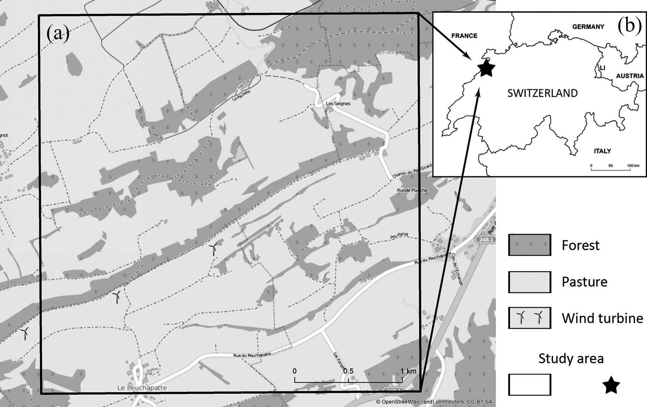
Study area: (a) general aspect (source: Open Street base map); (b) location within Switzerland (source: Esri world country boundary map).

Geologically, the study area belongs to the active belt of the folded and thrust Internal Jura mountains (upper most Miocen, ∼ 23 Ma), which is closely related to the push of the Alpine orogenic towards the Western Swiss Molasse Basin (Hindle and Burkhard, 1999; Sommaruga, 1999; Figure S1). The belt consists of Mesozoic thrust layers that are detached from a Permo-Carboniferous basement by Triassic evaporite layers (Hindle et al., 2000). According to Bourquin et al. (1946), the study area is crossed in the SW–NE direction by three anticlines and three synclines that model Jurassic and Quaternary deposits. Generally, the Jura range has remarkable parallel folded arches, indicating constant displacement trajectories, which are well emphasized by the presence of a series of escarpment lines that cross the area from SW to NE (Figure S2; Hindle and Burkhard, 1999). This impressive arc-shaped folding system has long been affected by intense erosion from the Pontian to Pliocene (Becker, 2000; Bourquin et al., 1946; Homberg et al., 2002). Currently, the folding system is a peneplain with a strong plateau characteristic. However, regional upliftings have reactivated the folds and renewed the relief.

Geomorphologically, the area’s landscape is an expression of a long and intense erosion of the Jurassic thrust and folds, resulting in a general aspect of a plateau that is crossed by a long parallel series of escarpment and caprocks. The long-time erosion influenced relief inversion – flattening anticlines and emerging synclines (Goudie, 2004), which are currently covered by forests and pastures (Figure 1). The steepest escarpments are related to the vertical layer area (Figure S1). On the topographical map (Figure S2), one can identify three types of escarpment areas with their corresponding slope inclinations and length. On the south-western edge of the steepest escarpment, two wind turbines are installed (Figure 1), indicating the good wind energy potential of the area.

III Data and methods

3.2 Fractional spline wavelets as a tool to extract multiscale landforms

We used fractional spline wavelets, which perform a discrete two-dimensional (2D) wavelet transform, using the cubic B-spline as the scaling function (Kalbermatten et al., 2012; Unser and Blu, 2000). This generated wavelet coefficients (based on a filter bank algorithm that allows for recreation of the signal using shifted and dilated versions of the wavelet) for each input signal from the DTM (Figure 2). The DTM decomposition performed with this type of wavelet provided the following four outcomes of the 2D signal: a 2 ⁱ resolution low-pass image, or generalized DTM, where i represents the decomposition level (i = 1,…, 4, with 1 corresponding to the original DTM) and the three images with high-pass detail coefficients following the horizontal, vertical and diagonal directions of the wavelets.

OPEN IN VIEWER

Figure 2.

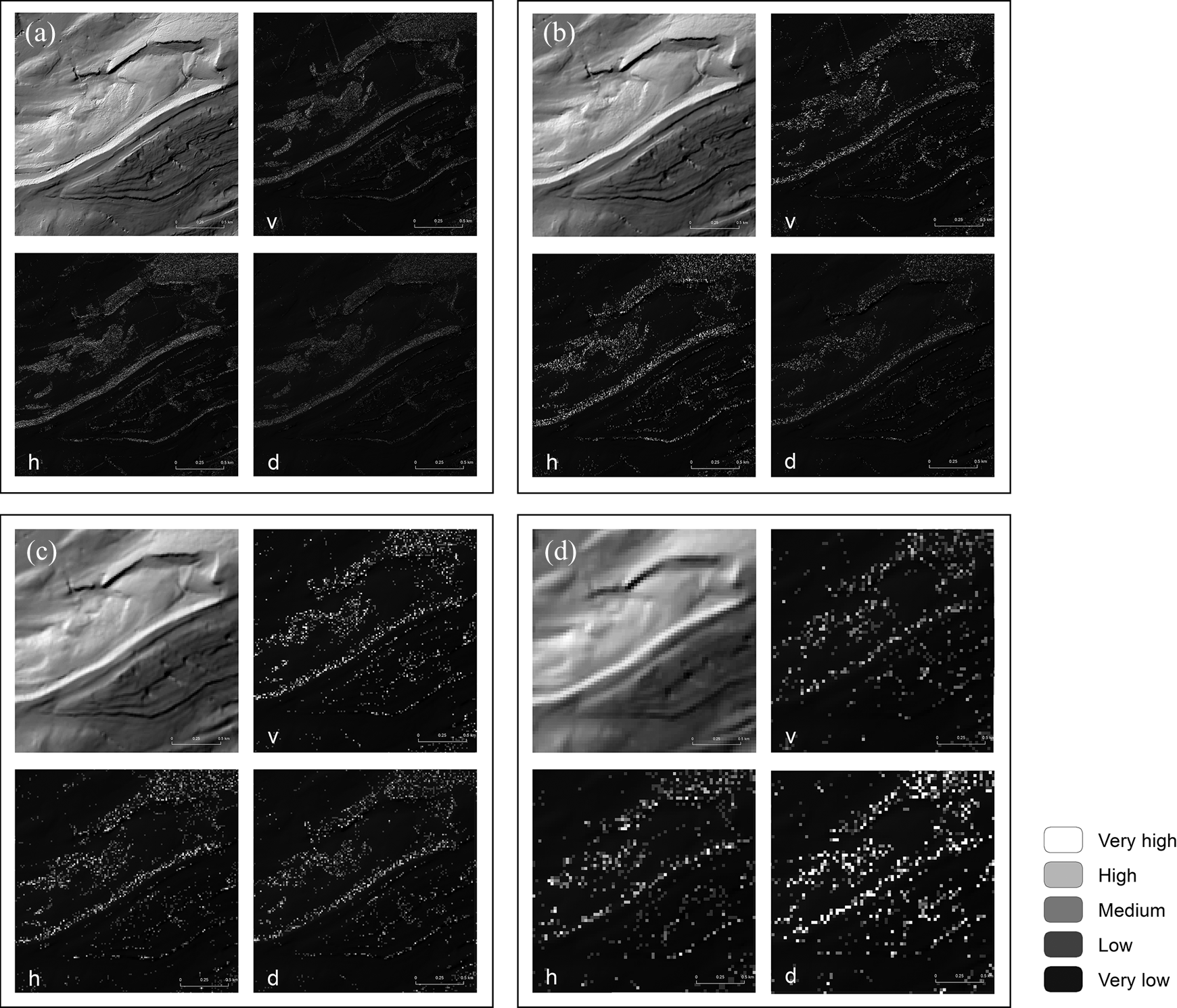
Multiscale high-pass wavelet coefficients maps: (a) 4-m resolution; (b) 8-m resolution; (c) 16-m resolution; (d) 32-m resolution. The multiscale high-pass wavelet coefficients are displayed according with their vertical (v), horizontal (h) and diagonal (d) direction. Note: for visualization reasons alone, we replaced the generalized digital terrain models from Figure 2 with their corresponding processed shade relief rasters.

We used MATLAB scripts (Blu and Unser, 2000; Unser and Blu, 2000), customized by Kalbermatten et al. (2012), to process the original signal c_i [k], i = 1, and the DTM at a 2⁽¹⁾ m resolution. In the following steps, through dyadic subsampling, the subsequent scales each had a resolution that was multiplied by a factor of 2, along with three different wavelet directions that are expressed by the high-pass coefficients of the (i + 1)^th decomposition level. The resulting low-pass images (c _{i+ 1}[2 k]) of the original DTM also integrate their directional high-pass coefficients (d) in the following three directions: vertical (d_{v ,i+1}[2 k]), horizontal (d_{h , i+1}[2 k]) and diagonal (d_{d ,i+1}[2 k]). Based on this dyadic subsampling, and in accordance with the total surface of our study area, a maximum number of four decomposition levels was sufficient to coherently display the resulting generalized DTMs and associated high-pass coefficient images with resolutions ranging from 4 m (the 2¹⁺¹ decay level) to 32 m (the 2⁴⁺¹ decay level).

Kalbermatten et al. (2012) described the specifics of wavelet transform by providing theoretical details and parameters to be used on the two linked functions. Furthermore, to enhance the terrain discontinuity and visibility of the geomorphological processes in the study area, we accumulated, via a bottom-up approach, the resulting directional high-pass coefficients that were detected by the fractional spline wavelet transform from 32 to 4 m (Kalbermatten et al., 2012). We recreated the specific subbands of the wavelet transform using an overlay raster operation in ArcGIS 10.1. At each decomposition scale, using the raster data geoprocessing technique, all of the resultant directional coefficient information was reassembled in one raster image with a cell size of 2 m as the original scale of the original signal (e.g., for the fourth decomposition level at the 32 m scale, we overlaid all resulting directional wavelet coefficients from 4 to 32 m, in one image raster of 2 m cell size resolution).

3.3 Mapping the geodiversity elements

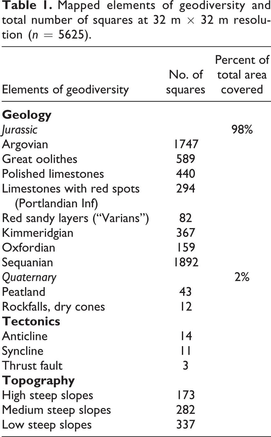
For this study, we used the geodiversity classification by Gray (2004) and Serrano and Ruiz-Flaño (2007b), which only contains topographical and tectonic elements (Table 1) from the study area. All elements were mapped using the available geological and tectonic maps (details in Section 3.1) as well as a shade map processed from the original DTM. Within the topographical map (Figure S2), we delineated three categories of steepness, according to the main directional elevation profiles and the 3D model of the study area, from high (>45^o and 40–60 m slope width) to medium (15–40^o and ∼20 m slope width) to low (5–10^o and ∼15 m slope width). These main topographical features overlap and follow the parallel disposal of the tectonic structure.

OPEN IN VIEWER

Table 1.

Mapped elements of geodiversity and total number of squares at 32 m × 32 m resolution (n = 5625).

Elements of geodiversity	No. of squares	Percent of total area covered
Geology Jurassic Argovian Great oolithes Polished limestones Limestones with red spots (Portlandian Inf) Red sandy layers (“Varians”) Kimmeridgian Oxfordian Sequanian Quaternary Peatland Rockfalls, dry cones Tectonics Anticline Syncline Thrust fault Topography High steep slopes Medium steep slopes Low steep slopes	1747 589 440 294 82 367 159 1892 43 12 14 11 3 173 282 337	98% 2%

To compute the total geodiversity map and geodiversity index map, we used the coarser grid resolution that was processed as with the wavelet decomposition in a 32 m × 32 m size window (grid cell) of the spatial grid for analysis (having a surface S = 1024 m²). The total geodiversity G_t was computed based on the following formula

G t = E g / S

1

(Hjort and Luoto, 2010), where Eg is the total number of geodiversity elements mapped on the geological and topographical maps per square unit of a 32 × 32 m² surface area (S). Furthermore, we refined the results obtained within the total geodiversity estimation of the study area by adapting the formula of Serrano and Ruiz-Flaño (2007a, 2007b) to compute the geodiversity index

G d = E g R w t / l n S

2

where Gd is the geodiversity index; Eg is the number of all physical elements composing the geodiversity (geological, tectonic and topographical; Table 1) at the square unit level; R_wt is the roughness coefficient of the unit, derived from the cumulative wavelet coefficient dataset or wavelet transform detected roughness (hereafter, WT roughness) at the fourth level of decomposition; and S is the surface area of the unit (m²). The use of WT roughness relied on the fact that the dataset was derived from high-resolution LiDAR measurements and, through data pre-processing, the noise was removed. As a result, one might assume that the information contained in these coefficients is related to the actual terrain variability.

The total geodiversity values range from very low geodiversity (one or no elements of geodiversity) to medium geodiversity (two different elements of geodiversity) to very high geodiversity (over three different geodiversity elements) per raster cell size. The geodiversity index computed values that were translated in intervals ranging from very low to very high.

3.4 Statistical modelling

Given the size of the dataset obtained through the conversion of grid data into vector data (>1.4 million records), we first performed an exploratory backward regression using the homonymous data-mining tool within Spatial Statistics from ArcGIS 10.1 (Esri, 2012). This statistical tool is performing well when processing large datasets and a selection of explanatory variables is needed. The outputs of the exploratory regression model were then refined with the Spatial Lag regression model by using the GeoDa open-source software (Anselin, 2005). The Spatial Lag regression model offers a detailed diagnostic on predicted values and residuals.

With the exploratory regression tool (Rosenshein et al., 2011) we investigated whether, at the coarser processed resolution of the area (32 m), the geodiversity index is explained by its defining parameters, namely geology, elevation, WT roughness and slope distribution data. The exploratory regression model helped to find the best possible combination of explanatory variables to be further used in the Spatial Lag regression model. It also provided a diagnostic evaluation of the redundancy, significance, performance and bias for all variables’ combinations. We only kept in the model variables that passed 50% of the significance test, the lower Akaike Information Criterion (AIC; Akaike, 1974), the maximum p-value and maximum variance inflation factor (VIF > 7.5; Kenneth et al., 2013), which is an index that detects multicollinearity (Meleg et al., 2013; Smith et al., 2009).

Subsequently, the explanatory variables exhibiting the best correlation within the exploratory regression model were used in the Spatial Lag regression model to examine the significant factors behind the spatial distribution patterns of data. The Spatial Lag regression model (3) is based on the maximum likelihood estimation by capturing the spatial dependence of data through a weight matrix

y = X β + ρ W y + ∊

3

where y is the dependent variable, X corresponds to the explanatory variables, β is a vector of unknown fixed-effects parameters, W is the weight matrix, ρ is the lag coefficient (a spatial autocorrelation parameter) and ε represents the vector of random errors (Anselin, 2005; Zhang et al., 2009). Following the same principle, we used the geodiversity index as the dependent variable and the best correlated parameters provided by the exploratory regression model as explanatory variables. We created a symmetrical weight matrix using the Euclidean distance as a function for searching the neighbouring features. To measure the fit of the model (Lee and Ghosh, 2009) we computed the AIC, the lag coefficient and the Schwarz Criterion (SC; Schwarz, 1978).

Spatial autocorrelation was tested for both the exploratory and Spatial Lag regression model at 32 m by using the Global Moran’s index coefficient (Anselin et al., 2006; Bivand et al., 2009; Goodchild, 1986). Kalbermatten (2010) suggests that spatial autocorrelation be computed over generalized elevation models using Global Moran’s I coefficient (ranging from −1 to 1). This coefficient’s values close to 1 indicate positive autocorrelation, while those near −1 indicate negative autocorrelation. We analysed the distribution of the standard residuals by taking into account that, under the null hypothesis of no spatial autocorrelation, the expected value E(I) of the Moran index is equal to −1/(n−1), where n is the number of tested samples (Goodchild, 1986).

We used the following tests to assess distribution of the standard residuals: AC_R (Global Moran’s I) and the Jarque-Bera’ p-values to measure the residual normality (R_N (J-B); Jarque and Bera, 1987) within the exploratory regression model, respectively the Univariate Global Moran’s I coefficient (AC) within the Spatial Lag model. We performed a randomization test (with 999 permutations) within the Univariate Global Moran’s I spatial autocorrelation (Anselin, 2005) that computes beside the value of I, the z-score, the expected value of Moran’s I and the pseudo probability. Finally, we computed the scatterplot matrix to display the best correlations among all of the factors that were used to explain the geodiversity index distribution within the 32 m resolution resulted dataset.

IV Results

Fractional spline wavelet filtering rendered four low-pass images (the generalized DTMs) at 4, 8, 16 and 32 m resolution, as well as the associated high-pass detail coefficient images in the vertical, horizontal and diagonal directions (Figure 2). For each decomposition level, a set of three directional images (diagonal, horizontal and vertical) resulted, which showed the distribution of discontinuities (high-pass coefficients) detected by the wavelet transform. According to the decomposition level and direction, these distributions indicate the size and depth of the topographical structures (Kalbermatten et al., 2012). We assumed that the first and second decomposition levels indicate, through their discontinuities, the small-sized elements comprising the geomorphological surface. For the first two decomposition levels, at scales between 4 and 8 m, the topographical structures are better detected in the horizontal direction. However, the south-eastern half of the area shows that these structures follow parallelism features that are recognizable on the geological map. The last two decomposition levels refer to wider and well-defined structures, which are formed by joining micro-structures. Furthermore, the third decomposition level (the 16 m resolution grid) shows a more balanced distribution of the discontinuities in all three directions as well as a higher homogeneity within the study area. The centre of the study area is dominated by a visible trace line with a high density of discontinuities, which are well outlined in all three directions. The density of discontinuities is the highest for the fourth decomposition level (at 32 m resolution). In addition, at this last decomposition level, the generalization process focuses on the centre of the study area, indicating a higher density of discontinuities on the diagonal direction image. At this decomposition level, the discontinuities dispersed more widely and heterogenically, describing well-defined structures.

The map of the cumulative high-pass wavelet coefficients (Figure 3) or the WT detected terrain roughness reproduces the magnitude of the detected discontinuities. We obtained four raster images containing the amplified discontinuities by overlaying the iterative results in the three directions and four coarser resolutions, which are based on the decomposition levels. The cumulative high-pass wavelet coefficient map indicates the terrain roughness within the study area as well as the size and depth of the present topographic structures. The topographical micro-structures that are detected by accumulating high-pass coefficients from the first and second level of decomposition (Figures 3(a) and (b)) are homogenously connected in patches within the north-east part of the study area and descend towards the lower central and western parts. In addition, in the central and the lower south-eastern parts of the study area, the parallelism of the underlying tectonics is marked by the presence of similar micro-structures. In the case of cumulated high-pass coefficients from the third and fourth levels of decomposition (Figures 3(c) and (d)), the topographical structures are better defined. The borders of the connected patches from the north-east and central-west parts of the study area are outlined by darker shades of grey as opposed to the surrounding lighter area. The lower half of the study area shows a widening of the parallel lines overlaying the synclines and anticlines, which are coupled with the appearance of similar features between these lines. In Figure 3(d), homogeneous areas of very dark shades of grey cover wide surfaces and frequently extend beyond a size of 32 m². The darker colour is an indicator of deeper topographical structures.

OPEN IN VIEWER

Figure 3.

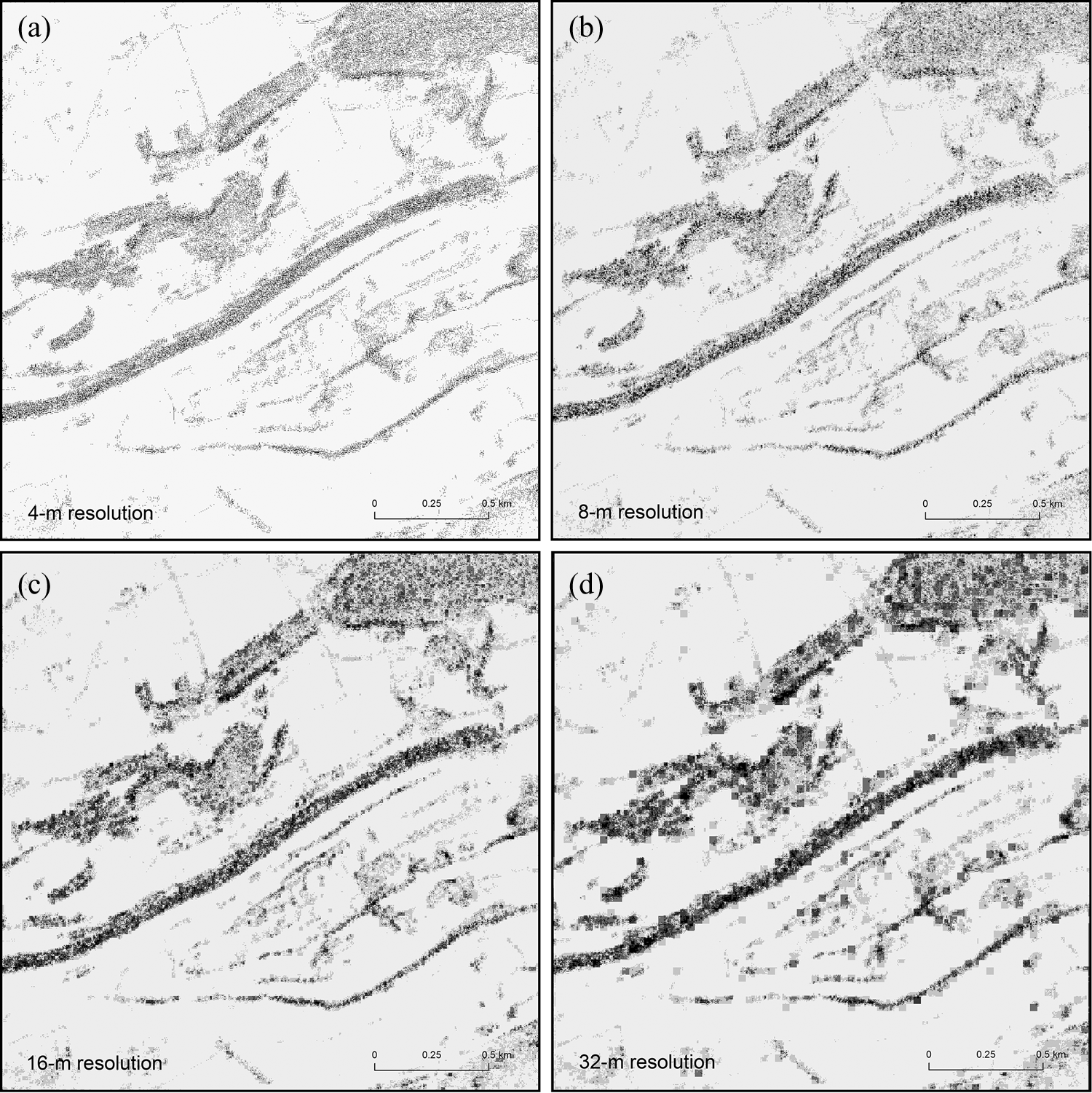
Cumulative high-pass wavelet coefficients map (wavelet transform detected roughness): (a) first decomposition level; (b) second decomposition level; (c) third decomposition level; (d) fourth decomposition level.

According to the geodiversity analysis, we mapped and quantified three main types of geodiversity elements (Table 1) and a total of 16 different geodiversity elements. The most abundant geological elements in the geodiversity analysis belong to the Jurassic structure (wide areas covered by Sequanian and Argovian materials). From the tectonic point of view, anticlines are dominant (including the refolded anticlines), followed closely by synclines. The topographical landscape is highly represented by low steep slopes. The geodiversity index map (Figure 4(b)) resulted in five intervals that vary from values of 0.5 to 7, which are illustrated with a colour map ranging from very low to very high geodiversity. According to these results, the geodiversity index shows a higher heterogeneity within the study area than the total geodiversity map (Figure 4(a)). On both maps (Figures 4(a) and (b)), the low and very low values of the geodiversity index have a wider distribution over the study area, while the medium to very high densities of elements are concentrated towards the central and southern parts. Furthermore, the geodiversity analysis also maps the parallel lines from the central and southern parts of the study area that correspond to the underlying tectonics.

OPEN IN VIEWER

Figure 4.

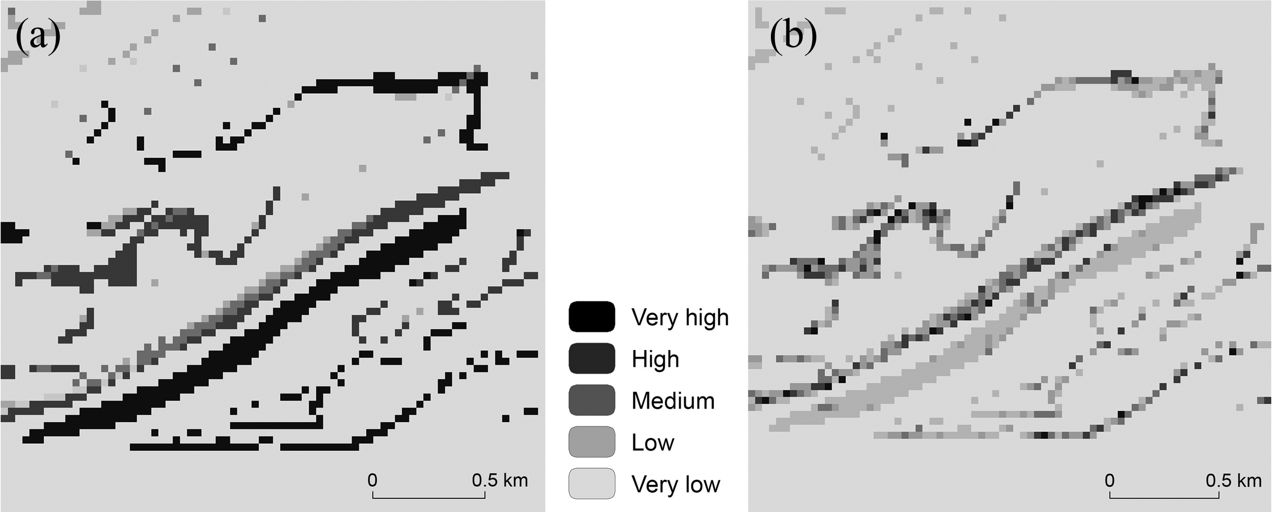
Geodiversity maps at 32 m × 32 m grid unit: (a) total geodiversity map; (b) geodiversity index map.

The exploratory linear regression model (Table 2) ran at 32 m resolution shows that the geodiversity index is best correlated with the WT roughness and slope data as follows: (i) a positive correlation with the slope dataset, indicating a higher geodiversity index with increasing slopes’ steepness; (ii) a positive correlation with the WT roughness values, resulting in co-increasing in geodiversity index values with terrain roughness values. Similar to the case of the exploratory regression, the Spatial Lag regression model (Table 3) indicates the same types of correlations of the geodiversity index with the best correlated explanatory variables, namely the WT roughness (positive) and slope data (positive), and a highly significant goodness of fit through the lag coefficient (ρ = 0.89; p < 0.0000). Both AIC and SC have high values (although AIC is significantly smaller than in the case of exploratory regression), not unusual for the large dataset we used (Anselin, 2005).

OPEN IN VIEWER

Table 2.

Summary of the exploratory regression model outcomes for the geodiversity index at 32 m.

Dependent variable	Predictors	Variable significance (%)	VIF	p-value	AIC	ACR (Moran’s I)	z-score	RN (J-B test)
Geodiversity index	Slope	100	1.19	<0.0000	17,688,969.2	0.9844	103.7658 Clustered distribution	<0.0000
	WT roughness	100	1.19	<0.0000				<0.0000

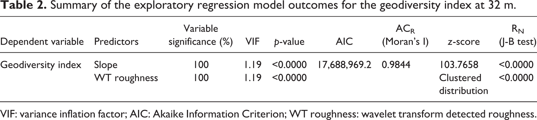
VIF: variance inflation factor; AIC: Akaike Information Criterion; WT roughness: wavelet transform detected roughness.

In the case of the exploratory regression model, AC_R assessed with the Global Moran’s I test (Table 2) has a value close to 1 (0.98), E(I) = −0.00017), and a significant R_N (J-B) test. The AC results obtained through the Spatial Lag regression (Table 3) yield the value of Univariate Moran’s I coefficient approaching zero, and a negative value of E(I). The z-score is also negative (−0.0218). The scatterplot matrix displaying all of the linear relationships used in the exploratory regression model at the 32 m decomposition level (Figure 5) suggests a strong correlation between the WT roughness and slope distribution.

OPEN IN VIEWER

Table 3.

Summary of Spatial Lag regression model results for geodiversity index at 32 m.

Dependent variable	Predictors	β	p-value	ρ	AIC	SC	AC (Univ. Global Moran’s I)	z-score	Pseudo p-value
Geodiversity index	Slope	0.84	<0.00000	0.89	14,700,300	14,700,400	0.0000	–0.0218 Random distribution	0.495
	WT Roughness	0.03	<0.00000

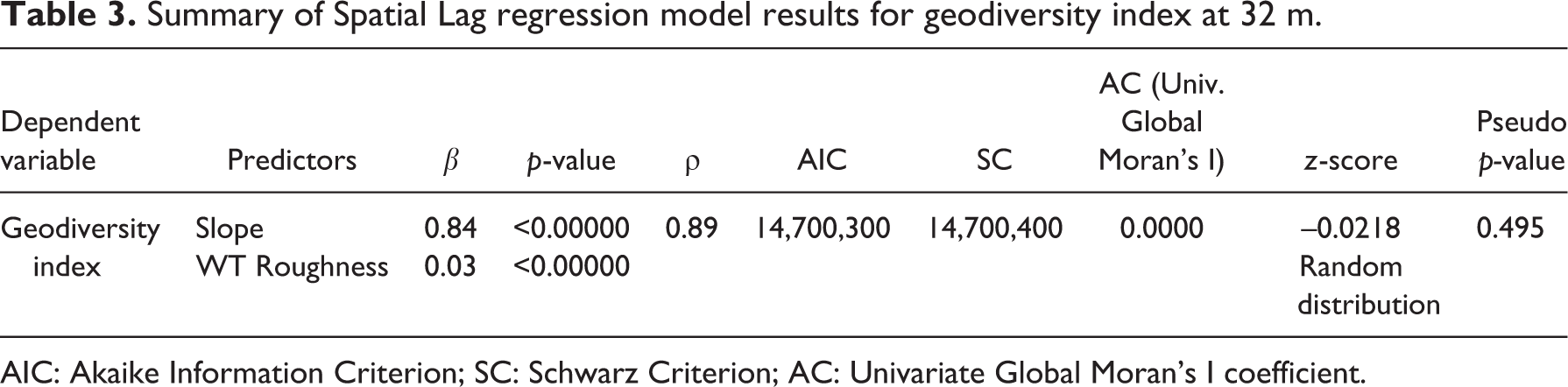
AIC: Akaike Information Criterion; SC: Schwarz Criterion; AC: Univariate Global Moran’s I coefficient.

OPEN IN VIEWER

Figure 5.

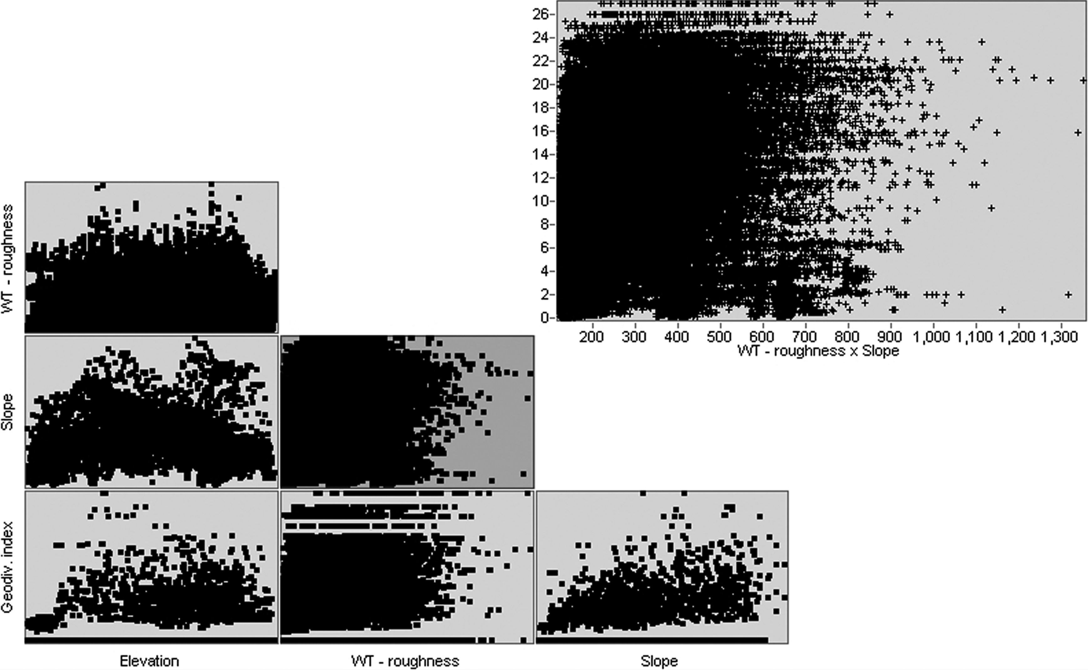
Scatter plot matrix displaying the linear relationships among the geodiversity index, slope, elevation and wavelet transform detected roughness.

V Discussion

At first glance, this case of a low mountain landscape represents terrain with very low geodynamics and long erosion periods. For such sites, it is a challenge to properly quantify and assess the geodiversity (Hjort and Luoto, 2010; Serrano and Ruiz-Flaño, 2007b). The method presented in this paper relies on an interdisciplinary approach. In this approach, WT-based image processing techniques were used to assess the geodiversity patterns of the landscapes by detecting the topographical features and underlying geology with the use of fractional wavelet transform.

High-pass coefficient maps and WT roughness maps (Figures 2 and 3) show important concentrations of terrain discontinuities that become less aggregated as the resolution decays. The flat areas alternate with steep areas as well as the dominant direction of the terrain discontinuities, following long parallel lines and indicating a geomorphological pattern. The Jurassic deposits (∼98% from the total surface) are cut by two thrust faults, separating the Inferior Portlandian limestone deposits from Sequanian limestones deposits (in NW) and the Inferior Portlandian limestone deposits from the Kimeridgian marls (in SE; Figure S1). Visually, the tectonic and geological evolution of the area is currently almost impossible to recognize at the surface because the terrain has been flattened through long-term erosion and is well-covered by forests and pastures (Figure 1). As a result, the maps depict the cumulative high-pass coefficient distribution, which was built with fractional wavelets, and helped us to extract elements related to the landscape structure that are not visible on the topographical and geological maps. Once the map resolution became coarser, we were able to identify the extent of these elements and their nested structures. Moreover, via wavelet transformation, we managed to identify the best defined tectonic slope in the central part of the study area (Figures 2 and 3). Fractional wavelet transform seems to be capable of reconstructing the geological history of the area and of clearly indicating the anticlines and synclines that cross the study area. These results are consistent with those of previous findings, such as those by Jordan and Schott (2005), who showed the ability of wavelet transform to detect geological faults and overlaid morphotectonic lineaments for a flat area.

Kalbermatten et al. (2012) used inverse wavelet transform to extract the decomposition levels of a terrain surface model with an active landslide. In our case, the study area does not reference any specific dynamics of geomorphological processes (the terrain does not contain dynamic structures), and we decided to enlarge the domain of the terrain roughness from 4 to 8 m resolution (considering the feature resolution interval from 1 to 20 m resolution). We kept the domain on relevant topographical structures and phenomena from 16 to 32 m resolution (with feature resolution ranging from 25 up to 60 m). Within this scale interval, we managed to capture and redefine very important tectonic lineaments and fractures that were otherwise unrecognizable to human perception. The small size study area, as well as the resolution of the original signal, indicates some difficulties and restrictions related to the number of decomposition levels as well as the display of the coarser results and their high-pass coefficient. Larger areas are more suitable to wavelet transform decomposition into coarser resolutions than 32 m to explore the extent and size of the topographical and tectonical features (Jordan and Schott, 2005; Kalbermatten et al., 2012). However, our study shows good results for detecting hidden topographical features when applied to smaller areas.

The total geodiversity map (Figure 4(a)) provides a rough estimate of the distribution of its elements. The geodiversity index map (Figure 4(b)) resulted in a more complex composition, as the computing formula (2) includes the roughness detected through wavelet analysis. Furthermore, the total geodiversity map alone does not accurately express local geodiversity. The geodiversity index (Gd) better refines the topography map with the help of WT roughness and changes the distribution of the areas with low to high values detected on the total geodiversity map (Figure 4(a)). All of these elements became more obvious on a multiscale approach, making it easier to quantify them and to statistically correlate them with their derived morphometrical parameters. As a result, the wavelet-based approach enabled the detection of hidden geodiversity. In turn, this could address further questions related to the presence of Jurassic limestones (as a determinant factor) and the probability of an active karst system. According to Figure 1, this slope is covered entirely by forest. When analysing the association of the multi-resolution wavelet high-pass coefficients (Figure 2) and multi-resolution WT roughness maps (Figure 3), the edge effect became obvious. At the surface, this effect is marked by separation between different types of land cover (forest on the steep tectonic slopes and pastures on the quasi-flat areas, Figures 1 and S2; Brierley et al., 2013). The hidden geodiversity, which was mapped with the help of wavelet transform to detect roughness, helps to complement traditional modelling approaches (Gray, 2008; Hjort and Luoto, 2010; Serrano and Ruiz-Flaño, 2007b) and shows promising results when applied to landscapes that lack obvious patterns (Cullum et al., 2015). The proposed method in this study offers in-depth interdisciplinary analysis through the multiscale approach, which involves terrain wavelet-detected discontinuity assessments.

At the coarse resolution of 32 m, the geodiversity index is best explained by the increase in the slope steepness, most likely resulted from the reduction of the similar neighbouring pixels. The steeper the slope, the higher the geodiversity index (Figure 5). The increase in the WT roughness values explains the increase in the geodiversity index, too. Previous studies also indicate that the slope and roughness are the main variables for mapping surface geodiversity using high-resolution elevation models (Hjort and Luoto, 2010; Serrano et al., 2009). The Spatial Lag method was suggested as the best option for regression models applied on large datasets (Anselin, 2005). The high significance of the two best correlated variables from the exploratory regression model was also maintained in the Spatial Lag regression model.

For the exploratory regression, the Global Moran’s I autocorrelation test resulted in a clustered distribution of the residuals (interpreted by a value of Moran’s I close to 1 and a high significance of the p-values of the R_N (J-B) test; Rosenshein et al., 2011). The Univariate Global Moran’s I (Anselin, 2005) ran in the Spatial Lag regression model showing negative values for both the estimates and z-score, suggesting no spatial autocorrelation in the distribution of the residuals (Goodchild, 1986). Furthermore, this represents a confirmation of the presence of hidden geodiversity when the slope and WT roughness are positively correlated.

VI Conclusions

Geodiversity analyses offer a complete inventory of abiotic layers. A high geodiversity value is associated with landscapes that have variability in geological, geomorphological, hydrographical and pedological elements. Quantifying geodiversity is necessary for landscape management as well as for land use planning. In this study, we proposed a tool to map geodiversity that can quickly and accurately estimate landscape variability in terms of geodiversity patterns and elements (i.e., related to tectonics and topography). This tool combines high-resolution terrain models and image processing wavelet-based techniques to detect the geodiversity patterns of a landscape. Our approach relies on the capacity of wavelets to accurately “read” the non-stationary nature of natural phenomena and geomorphological processes within high-resolution terrain models.

The multiscale wavelet-based model was tested on a small area from the Swiss Jura range. It was able to detect important geodiversity patterns, such as nested and hidden topographical features and geodiversity elements that are not directly visible on very high-resolution DTMs. The method showed promising results related to the identification of tectonic and topographical elements. Combined with other datasets (e.g., pedology and hydrography) and suitable techniques, it was able to better link geodiversity and biodiversity. Moreover, the underlying geology was better emphasized with the use of the fractional spline wavelet analysis decomposition.

Our research tool is relevant for detecting and assessing the hidden geodiversity of a landscape as a key element to better preserve its most important features through precise landscape planning and management guidance.