
Abstract
Turbidity of water due to the presence of suspended sediment is measured and interpreted in a variety of ways, which can lead to the misinterpretation of data. This paper re-examines the physics of light scattering in water, and exposes the extent to which the reporting of turbidity data is inconsistent. It is proposed that the cause of this inconsistency is the fact that the accepted turbidity standards USEPA Method 180.1, ISO 7027 and GLI Method 2 are mutually inconsistent, as these standards give rise to a large number of measurement units that are not based on the optical properties of light absorption and scattering by suspensions in water, but by the arbitrary definition of the degree of turbidity being due to a concentration of formazin or other similar polymer-based calibration standard. It is then proposed that all turbidity-measuring devices should be calibrated with precise optical attenuators such as neutral density filters. Such calibration would allow for the definition of a beam attenuation coefficient for every turbidity-measuring instrument which would be cross-comparable with any other instrument calibrated in the same way. The units for turbidity measurements should be based on attenuation and reported as dB m−1. It is also proposed that a new standard should be drafted according to this attenuation-based method, and this new standard should also define the nomenclature for reporting data collected at any specific scattering angle in terms of an attenuation in dB m−1. The importance of multi-parameter turbidity measurements for the improvement of the quality of turbidity data and the application of parameter-rich data sets to new methods of sediment characterization are discussed. It is suggested that more research into multi-parameter turbidity measurements is needed, as these new methods will facilitate an increase in parity between turbidity and suspended sediment concentration, a relationship that is subjective.
I. Introduction
The term ‘turbidity’ is used widely throughout the physical sciences, and is interpreted in different ways in different contexts. It is commonly used to describe the optical clarity of a fluid (e.g. the atmosphere), but for the purposes of this paper it refers to another common usage of the term which is the optical clarity of water. The presence of suspended particulates, dissolved inorganic chemical species, organic matter content and temperature can all affect the turbidity of a body of water. Investigators from different fields (wastewater treatment, drinking water quality, forestry, civil engineering, aquaculture and ecology), and from the sub-disciplines within physical geography (fluvial, marine, glacial, coastal and estuarial), use turbidity measurement as a surrogate relative indicator of some other physical property, typically suspended sediment concentration (SSC) or total suspended solids (TSS). The amount of literature available on the subject of water turbidity is large, and a number of reviews have already been undertaken by investigators from some of the sub-disciplinary groups (Bilotta and Brazier, 2008; Davies-Colley and Smith, 2001; Kerr, 1995; Ziegler, 2002). There is however, some disagreement about what turbidity actually means, partly due to the different sub-disciplinary contexts in which the term is used, and partly because of the way in which the various measurement standards are assumed to be based on a correct a priori understanding of the physical processes of light-scattering and absorption.
Why is turbidity measurement important? The answer to this question depends on the perspective of the investigator. Some researchers are purely interested in the effect that the attenuation of light has on, for example, aquatic ecosystems, so that knowledge of the mass concentration of the suspended particles is not always the primary concern. In this case other parameters of interest include the reduction of visual range in water (affecting the ability of predators to hunt), and the amount of light available for photosynthesis (Bilotta and Brazier, 2008). Other investigators are concerned directly with the study of sediment-transport processes, in which case knowledge of the mass concentration of the suspended particles and other parameters such as the particle size distribution (PSD) is highly desirable for a number of reasons. Turbidity measurement is important in this context, as although the turbidity measurement itself is heavily biased by the PSD (Gippel, 1989), it is not specifically designed to provide detailed information about the PSD. For example, knowledge of particle size is important as the transport of fine sediment derived from different land uses through catchments will impact directly on ecosystem services, such as the provision of drinking water. Fine sediment delivery into river systems is also known to cause problems such as irritation to fish gills whilst it is in suspension (Davies-Colley and Smith, 2001). Bilotta and Brazier (2008) summarize the effects of what they refer to as suspended solids (SS) on periphyton and macrophytes, invertebrates and salmonid fish species. The displacement of many fish species can often be due to an increase in turbidity caused by the cumulative effects of fine sediment introduced into the riparian environment as a direct result of human activities such as deforestation (Kerr, 1995), or by natural events such as sediment transport by stormwater runoff. The use of turbidity measurement as a surrogate indicator for parameters such as SSC has been explored by many researchers, as reviewed by Ziegler (2002). It has been shown that the PSD of a homogenous sediment can vary temporally from its source (e.g. hillslope runoff) as it is transported through a catchment into a stream, due to a variation in the relative proportion of aggregates (flocs) present in the measured flux (Slattery and Burt, 1997). Therefore knowledge of how the PSD varies dynamically in this fluvial context due to variability in the degree of flocculation (DOF) is important for the study of the transport processes of both sediment and organic species in flocs (Williams et al., 2007). There is clearly some variation in the importance given to the parameters of turbidity by the different sub-disciplinary groups, and so the aim of this paper is to evaluate how relevant turbidity measurement is to the study of sediment-transport processes specifically, and to propose methods for the improvement of the measurement and reporting of turbidity in a general context. The steps required to achieve this evaluation are given by the following list of objectives: To analyse critically the measurement methodologies described in the literature including any inconsistencies in nomenclature of measurement principles. To review briefly the physics of light absorption and scattering processes in water in order to provide an underpinning for the discussion of the definition of terms according to various investigators from different sub-disciplinary groups. To present a critique of the measurement units, calibration methods and standards applicable to the measurement of turbidity, SSC and TSS, and to examine the origins of the relationship between turbidity measurements and the implied properties of suspended sediment. This step is vital because the cross-comparability of turbidity data obtained in the field is often invalid due to a widespread reliance on the assumed integrity of Formazin calibration methods. To propose, based on objective 3, that a new turbidity instrumentation standard is required, and to describe its fundamental content.
II. Turbidity measurement principles and nomenclature
The measurement of turbidity is split into two basic methodologies: turbidimetry, in which the degree of transmission of light is determined, and nephelometry, in which the degree of light-scattering is evaluated (see reviews by Lawler, 1995, and Ziegler, 2002). This division has its roots in the mathematical descriptions employed to model the various phenomena. In the case of turbidimetry, the appropriate theories are due to Beer (1852) and Lambert (1760); as for nephelometry, many theories and models have been developed to describe a range of scattering processes, and these models are mostly derived from Mie theory (Mie, 1908). Nephelometry itself is sub-divided into three further categories which are forward-scattering, side-scattering and back-scattering. Side-scattering is generally accepted to be a measurement angle of 90° to the incident beam, although the existing standards impose different upper and lower bounds on that value (see Table 3). Forward-scattering (0° < θ < 90°) and back-scattering (90° < θ < 180°, often referred to as optical back-scattering or OBS) however, do not have a well-defined relative measurement angle. Different instruments employ different measurement angles, and these values are not always reported.
Before continuing with the discussion another ambiguity in terminology must be addressed. The definition of the scattering angle in terms of where the 0° position is located spatially also varies throughout the literature (Table 1). For example, in some cases a forward-scattering angle is stated, which implies that the transmitted (direct) beam is located at 0° (Agrawal et al., 2008; Jansson, 1992). Contradictory to this position, Bilro et al. (2010) define the transmitted beam as being located at the 180° position. In one instance two contradictory diagrams are presented in the same paper (Sadar, 2004, pp.8–9), and in many other cases the scattering-regime nomenclature is not associated with a specific scattering angle (e.g. Fugate and Friedrichs, 2002).
A selection of turbidity literature references illustrating the ambiguity associated with the assignment of scattering-regime nomenclature to the actual scattering-angle.
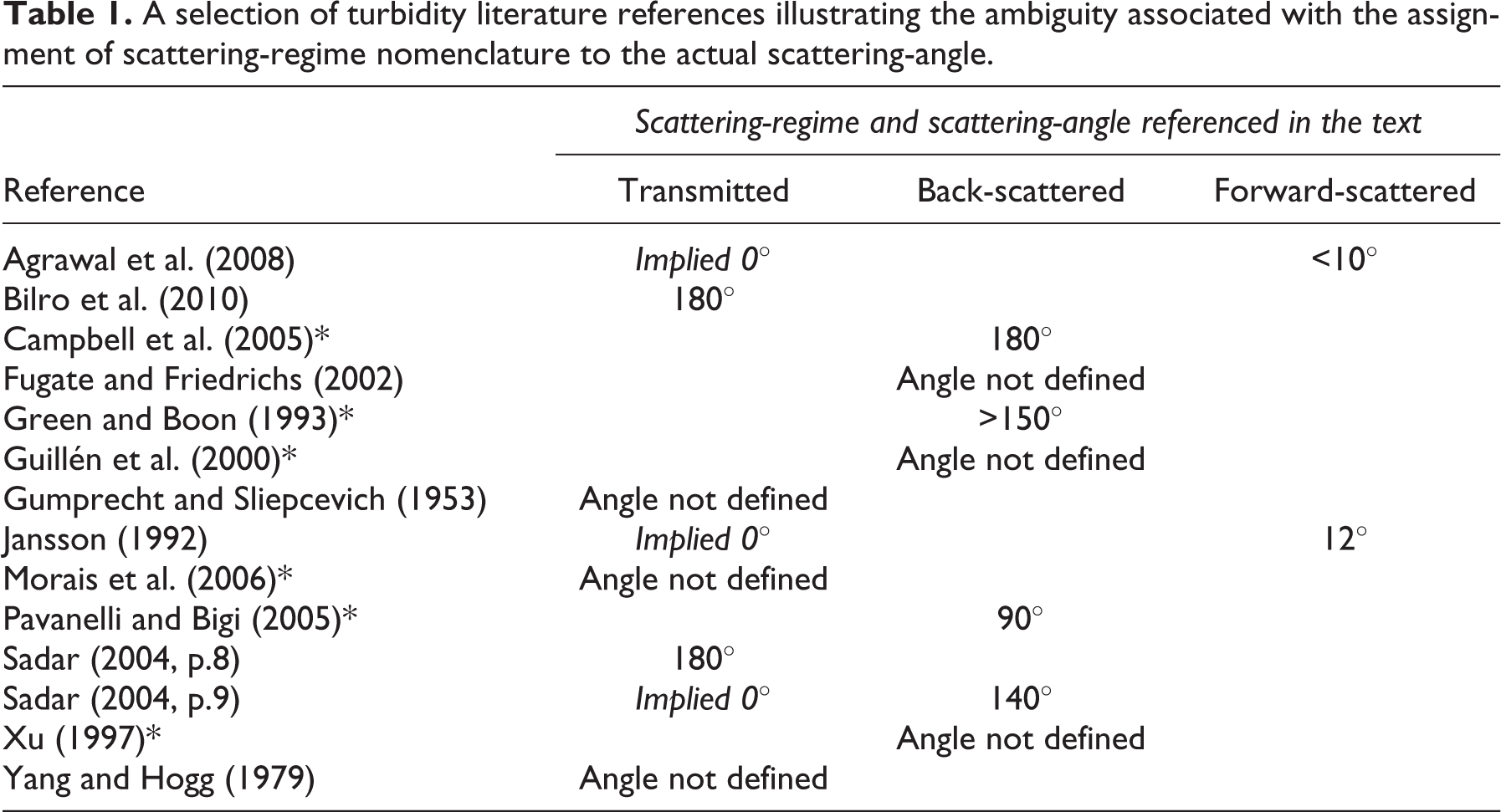
The interpretation that is adopted throughout this paper is that the scattering-angle is specified in terms of a detector placed at a position with respect to the incident beam after a physical interaction has occurred in the sample, i.e. the direct beam detector is placed at the 0° position (denoting ‘pure’ attenuation measurement), forward-scattering detectors are placed anywhere from 0° ≤ θ < 90°, a side-scattering detector is placed at exactly 90°, and back-scattering detectors are placed at 90° < θ ≤ 180°.
III. The physics of light absorption and scattering through turbid water
1. A brief review of optical theories
To understand the physics of light scattering by particles suspended in water, it is necessary to have some knowledge of the mathematical models employed to describe the various absorption and scattering processes. Fundamental theory and mathematical model development are continually progressing in this area, but the basic points of interest pertinent to the understanding of turbidity in water for the practical investigator are summarized in this section. Three main theories are discussed: Rayleigh theory, Mie theory and geometric optics. Also discussed are two theories that can be considered as approximations to Mie theory for specific conditions. These are the Fraunhofer diffraction theory (FDT) and the anomalous diffraction theory (ADT) of Van De Hulst (1957). The reason that these two theories are considered here is that they both yield computationally fast algorithms that are utilized by laser-based particle-sizing instruments. These instruments are used widely in suspended particle analysis (organic and inorganic) both in situ and off-line in laboratories, and are extensively employed for suspended sediment characterization.
Rayleigh and Mie scattering
The third Baron Rayleigh formulated his scattering theory to account for the blue colour of the sky (Strutt, 1871). Rayleigh scattering involves particles that are much smaller than the wavelength of the incident light, and are also defined as being optically soft – meaning that the particles are limited to having a refractive index very close to 1 (air molecules in the case of Rayleigh’s model). Rayleigh demonstrated that scattering from small particles is strongly wavelength dependent in favour of the shorter wavelengths and is spatially isometric (i.e. scattered equally in all directions), hence the blue colour of the sky. He determined that this blue colour is predominant because the scattered light intensity is inversely proportional to the fourth power of the incident light wavelength, i.e. the shorter wavelengths of light (e.g. blue end of the visible spectrum) are scattered more readily than the longer wavelengths of light (e.g. red end of the visible spectrum).
Gustav Mie originally developed his theory to explain the colouration of metals in the colloidal state (Mie, 1908). Mie theory successfully explains the dominance of forward scattering where particles are of a similar size to or larger than the incident wavelength of light, unlike the case of isotropic scattering of light by much smaller particles as in Rayleigh scattering.
In order to get some sense of the particle size ranges that are applicable to the different scattering regimes it is first necessary to define the dimensionless size parameter x,
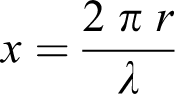
where r is the spherical particle radius (m) and λ is the wavelength of the incident light (m). Figure 2 shows how the forward-lobed nature of a set of light intensity distribution functions develops as x increases from 0.1 to 10. These spatial intensity distribution functions are also known as scattering phase functions, which are calculated using Mie theory.
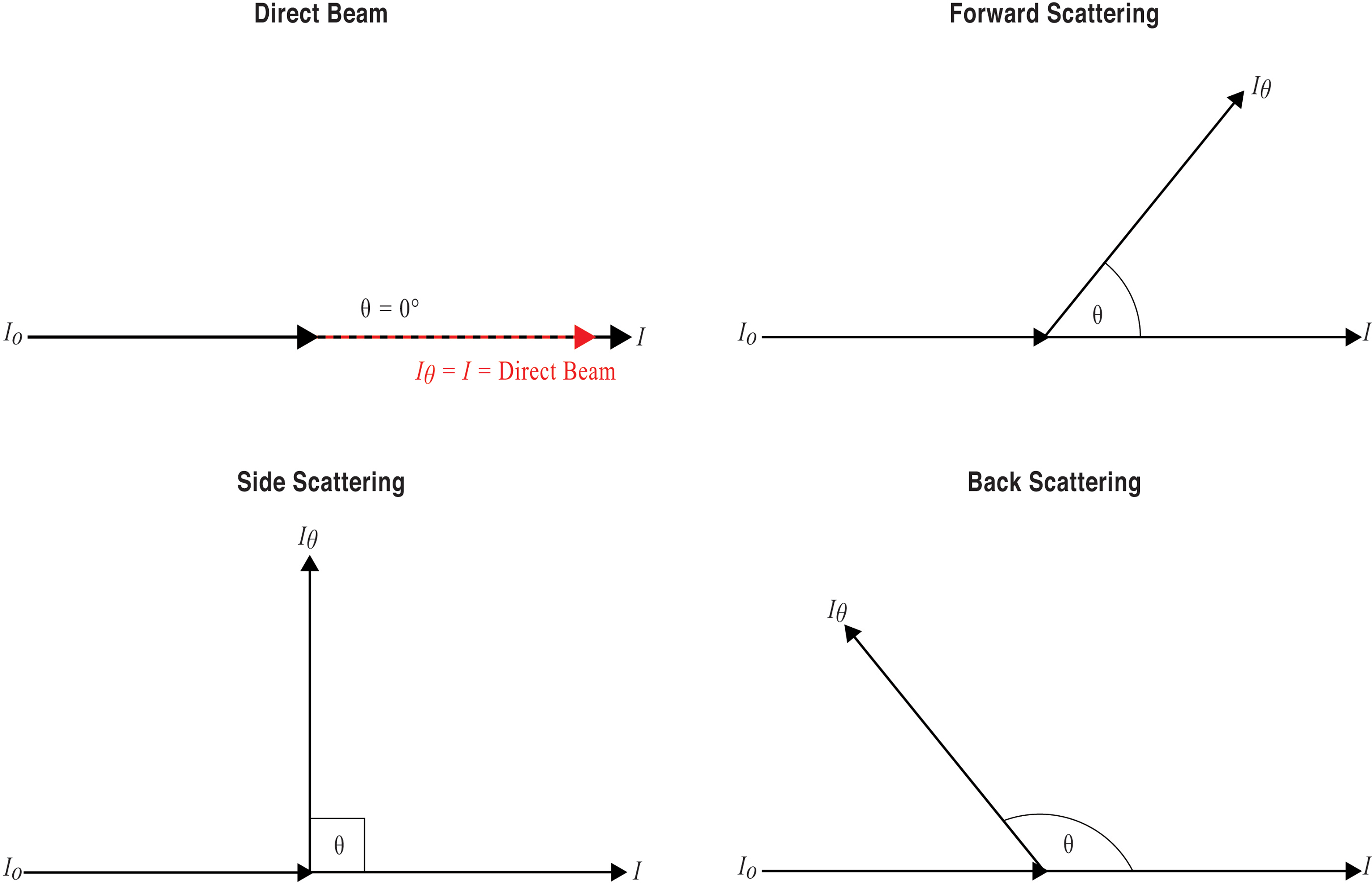
Illustrations of the light-scattering angle convention: the ‘direct beam’ where I θ = I, forwardscattering, side-scattering and back-scattering. The incident beam is denoted I 0 and the direct transmitted beam at 0° to the incident beam is denoted I. The scattered beams are denoted I θ, where θ is the scattering angle with respect to the incident beam.
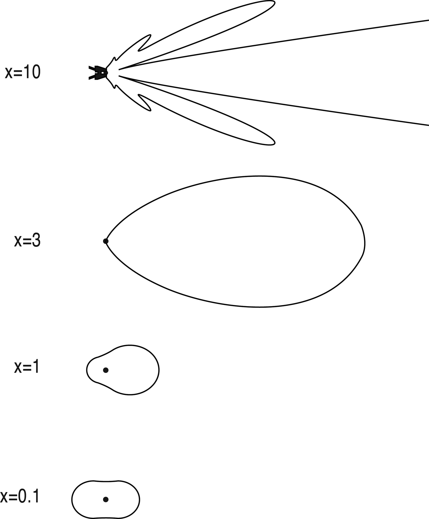
Scattering phase functions derived from Mie theory, with light incident from the left of the diagrams. Forward scattering becomes more pronounced as x increases.
Geometric optics
Geometric optics, otherwise known as ray optics, describes the light traversing a medium in terms of a straight path (hence ‘ray’). It explains refraction, in which there is a change in direction of a light ray at the interface between two regions with differing refractive indices. It also accounts for reflection and absorption, and is best applied in situations where the wavelength of light is much less than the size of the scattering particle. Figure 3 depicts a simplified diagram of scattering and absorption processes of a particle suspended in water as viewed from the perspective of ray optics.
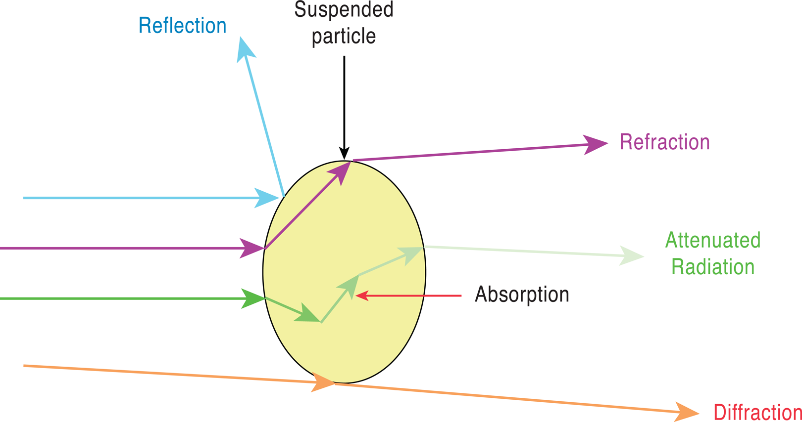
The scattering processes of reflection, refraction and diffraction, and the attenuation process of absorption of light due to a particle suspended in water.
Fraunhofer diffraction theory (FDT)
Fraunhofer diffraction occurs at small angles to the forward-scattered beam, i.e. <30°. Under these conditions of wavelength and scattering angle, FDT is a useful approximation to Mie theory, and is popular due to the relative simplicity of its algorithms. Due to the wavelength and particle size restrictions FDT cannot be applied to sub-micron sized particles. For example, the smallest sized sediment particle that could exhibit Fraunhofer diffraction when illuminated by a beam of red light (wavelength 630 nm) would be 6.3 µm, i.e. well above the sub-micron size limit.
Anomalous diffraction theory (ADT)
ADT (Van De Hulst, 1957) is a computationally efficient method by which the scattering from small particles can be modelled. The caveat is that the particles must be optically soft as in Rayleigh scattering (i.e. they must have a refractive index close to 1), and they must also have a large size parameter x >> 1.
2. The single scattering albedo
The single scattering albedo, denoted ω, is a useful unitless quantity defined as the ratio of scattering efficiency to total extinction efficiency. If the attenuation observed by a detector placed in the ‘direct beam’ configuration as in Figure 1 was due entirely to absorption, then ω = 0. When the observed attenuation is due to scattering processes alone, then ω = 1. The scattering albedo is useful when describing the particle size range that can be effectively modelled by the various regimes (Rayleigh, Mie, etc.). A graph of scattering albedo (ω) versus size parameter (x) is presented by Moosmüller and Arnott (2009, p.1031), which shows the particle size ranges covered by Rayleigh and Mie theory for particles with a refractive index of 1.55 (similar to that of silica). On this graph, the approximate scattering-model regime boundaries are observed, as shown in Figure 4. The large particle limit of Mie theory is also shown, and the size parameter at which Mie theory converges with this limit is the point at which geometric optics (not shown on the graph) becomes an alternative scattering model (at x ≈ 2000).
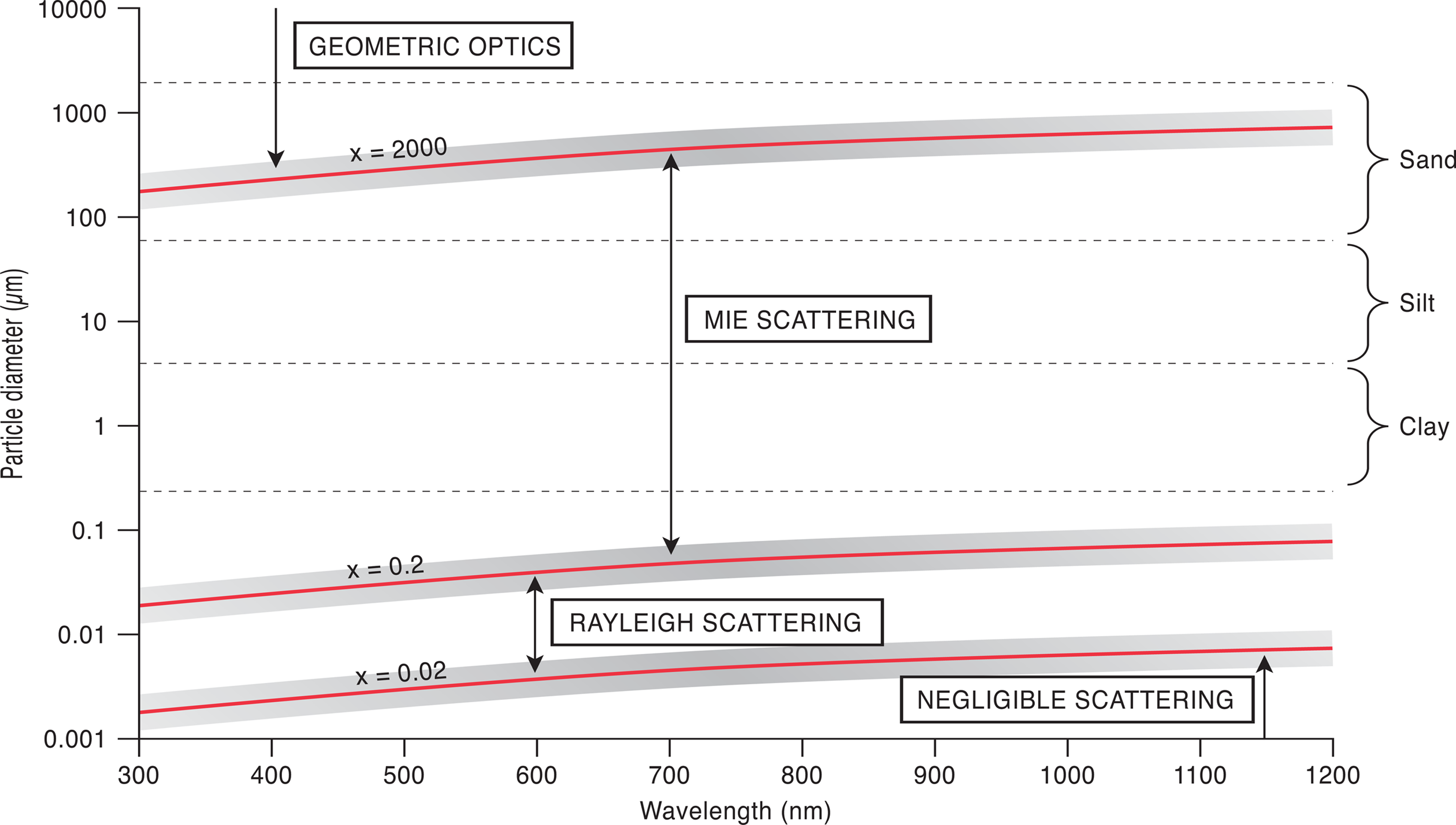
Light scattering theory regimes as a function of particle diameter and wavelength of light. Also shown are sediment particle size bands according to the American Geophysical Union Sediment Classification System.
IV. Light absorption and scattering by suspensions in water
In the terminology of physical optics absorption is a non-parametric process, i.e. one that is inherently lossy – meaning that energy is dissipated in the absorbing medium. The parametric processes that are to be considered do not involve any imparting of energy to the physical system through which the radiation is traversing, i.e. the wavelength of the scattered light is not altered (elastic scattering). The pertinence of these (and other) theories to the study of suspended particles in general, and suspended sediment specifically, must be considered. Rayleigh theory is applicable to small, non-absorbing (dielectric) spherical particles. Mie theory is the most ubiquitous of the models that is applied to the study of light scattering by suspensions in water. It represents a general solution to scattering from absorbing or non-absorbing spherical particles, with no limits on particle size. Rayleigh theory is less complex to apply than Mie theory, but is limited to small particles. The dimensionless size parameter x (equation (1)) for the scattering regimes, and the equivalent approximate particle size ranges are:
The graph of wavelength vs. particle diameter (Figure 4) shows the accepted boundaries between the various scattering regimes, as adapted from Lelli (2014) and confirmed by Moosmüller and Arnott (2009). Also plotted on the graph are the clastic sediment size ranges that are of interest in this paper.
Interpretation of this plot must however be considered carefully, as the data it represents are limited to a single scattering event from a purely spherical particle. The regime boundaries located at x = 0.02, x = 0.2 and x = 2000 (Lelli, 2014; Moosmüller and Arnott, 2009) are not strict demarcation lines (i.e. Mie theory includes Rayleigh theory as x → 0), but are there to suggest the generally accepted view of where the various models are used with respect to particle size parameter x. These boundaries should be considered to be somewhat blurred when applied to multiple-scattering from non-homogenous suspended sediment particles. Considerable model development is needed to account for scattering from large, non-spherical sediment particles. This work will lead to a redefinition of the scattering regime boundaries as depicted in Figure 4, with new models specific to suspended sediment being represented on the graph. There would also be one omission from the graph, namely Rayleigh scattering. As far as light scattering from suspended sediment is concerned, this theory has no application due to the restrictions in particle size (i.e. very small: <76.4 nm) and refractive index (i.e. n ≈ 1). Although Mie theory is limited to small, spherical particles only, it has many extensions that describe much more complex scattering regimes (including multiple-scattering and scattering from small non-spherical particles), and also simpler scattering regimes such as FDT (valid for particle diameter d ≥ 10λ, and scattering angle θ ≤ 30°). Other theories such as ADT which as with Rayleigh theory was originally designed for optically soft particles (but in this case with a large x value), are also adaptable to cope with higher refractive indices and non-spherical particles (Liu et al., 1998).
There is clearly a need to find a light-scattering model framework that is consistent with both small and large particle scattering, and which is also extensible to many-particle analysis. In the case of back-scattering from suspended sediment it has been shown that the reflectivity of the sediment also has a direct effect on the scattered light intensity (Sutherland et al., 2000), suggesting that geometric optics may play a part in future model development. Without a comprehensive understanding of the complex manner by which particle size, shape and concentration affect the absorption and scattering of light, it will not be possible to interpret what a turbidity measurement actually means.
V. The definition of the beam attenuation coefficient
The attenuation coefficient, Σ, is commonly referred to as the beam attenuation coefficient (BAC) in the turbidity literature, but these two quantities are defined in different ways by different authors. It is important that the ambiguities in both the definition and application of the BAC as a method for comparing turbidity data obtained by different methods are appreciated, as these ambiguities can lead to the misinterpretation of that data. The following discussion focusses on how the a priori Σ is defined, and then leads on to a definition of the BAC as an expression of Σ in terms of observable quantities, i.e. a measured attenuation and the optical path-length of the measurement instrument.
1. The attenuation coefficient Σ
Light is absorbed by water and this absorption is a function of the wavelength of the incident light (Figure 5). The strongest absorption occurs at a wavelength of λ = 417.5 nm (Pope and Fry, 1997) which gives a maximum reduction in transmitted light intensity of 0.05% over a distance of 0.1 m, which is the typical limit to the optical path length of existing turbidity instruments. As this is the worst-case scenario, the absorption of light by water is considered to be negligible in the context of turbidity measurement.
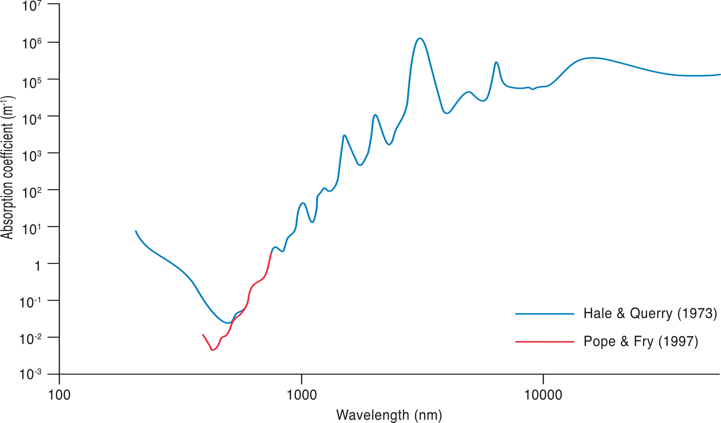
The light absorption spectrum of water. After Hale and Querry (1973) and Pope and Fry (1997).
Light is also absorbed by any other material that may be suspended in the water. In order to determine practically a value for absorption it is necessary to measure the amount of light transmitted through a given sample of water. This is termed the transmittance, T, which is defined as the ratio of the transmitted light intensity I to the light source intensity I0 , and has units of Wm-2. The transmittance is also related to the optical depth, τ (effectively the opacity of the medium), and the absorbance, A:
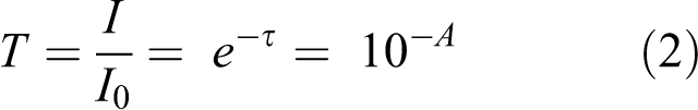
A quantitative measure of the optical depth τ can be expressed in terms of the natural logarithm of the transmittance or in terms of the absorbance:

This in turn leads to a definition of absorbance with units of the neper:

or in terms of the base-ten logarithm yielding a decibel quantity:

This definition of absorbance as a logarithmic function of transmittance is useful as it facilitates a linear relationship with the optical path-length. When a linear relationship between transmittance and path-length is established it then becomes theoretically easier to relate the absorbance to the concentration of a suspension, which will consequently itself be a linear function.
The a posteriori description of the attenuation of light through a homogeneous medium is credited to Bouguer (1729) and is also associated with Lambert. It has been called Bouguer’s law, Lambert’s law (Lambert 1760) and the Bouguer–Lambert law. It states that the attenuation is proportional to the distance travelled through the absorbing medium. The extension to this law which includes a term for the concentration of absorbers is known as Beer’s law, or more ubiquitously as the Beer–Lambert law, which states that the attenuation is proportional to the concentration of the absorbers (Beer, 1852).
The Beer–Lambert law allows the absorbance to be stated under ideal conditions, including the assumption that there are no scattering processes occurring in the sample, and that the attenuation is linear along the light path. This law enables the absorbance to be directly related to the concentration of absorbers, c, and the path length l:

where ∊ is the absorptivity (m2, or m2 kg−1) of the absorbers in suspension, and is a constant dependent on the physical properties of the absorbers (i.e. dielectric properties). Equation (7) expresses the same quantity as a transmittance:

When defined in these terms, the attenuation coefficient Σ can be stated as the product of the absorptivity and the concentration of the absorbers:

Substituting equation (8) into equation (6) gives the absorbance in terms of the attenuation coefficient:

The attenuation coefficient can be expressed in Naperian terms or as a decadic quantity (i.e. in decibels). The measured luminance (Cd m−2) represents the power delivered by the transmitted light beam per unit area. In electronic design it is more common to use decadic terminology to specify measurement instrument parameters such as those used for the determination of light attenuation. If equation (7) is substituted into equation (5), then the absorbance can alternatively be stated in decibels:


It is worth noting that the absorbance A is a dimensionless parameter, and the attenuation coefficient Σ has units of reciprocal length (m−1). However, the absorptivity ∊ may have different units depending on the context in which the concentration c is expressed (equation (11). For example, in the case where the concentration is simply the number of absorbers N per unit volume, then the units of concentration are reciprocal volume, i.e. m−3 or l−1. Therefore, absorptivity ∊ in this instance has units of m2. In the case of suspended sediment, the absorptivity ∊ would have units of m2 kg−1. It is important to recognize the units stated for absorptivity, as other nomenclature could potentially refer to the same physical quantity. For example, the mass attenuation coefficient used in chemistry also has units of m2 kg−1. Hence it is prudent to examine the mathematical definition being used within a given text to determine what physical quantity is actually being discussed, and not to rely on the accuracy of the nomenclature at all. Another example of ambiguous nomenclature is highlighted by Figure 5, which shows the graph of the light absorption spectrum of water. The range of this function is referred to as the absorption coefficient, and as it has units of reciprocal length (m−1) it is equivalent to the Σ of this discussion (i.e. the attenuation coefficient). This multiplicity of measurement units has the potential to cause confusion, since the absorption coefficient has the same units as the attenuation coefficient Σ. This is an important point as absorption is not the same as attenuation. Attenuation is the end result of the effects of the physical properties of the medium on the propagation of the light waves, and represents a loss of measureable light intensity. Any measured attenuation cannot be presumed to be due to absorption alone (Figure 3). Scattering of light can occur in all directions, and reflection and refraction of light can also distort any attenuation measurement. For example, Gumprecht and Sliepcevich (1953) suggested that forward scattering can distort a true attenuation measurement by adding to the transmitted light intensity observed by a detector. This forward-scattering component is referred to as the extinction coefficient by Clifford et al. (1995, p.774), who describe it as ‘the re-formation of light after scattering behind the particle’, and attribute this effect to the presence of suspended particles of diameter less than approximately 4 µm.
2. BAC – the beam attenuation coefficient
The attenuation coefficient Σ is defined for ideal conditions, i.e. situations in which the attenuation of light obeys the Beer–Lambert law and is thus concerned with absorption only, although some definitions of BAC include a term for light-scattering (Kirk, 1985). However, light-absorption cannot be measured directly; only the attenuation of a light source can be determined by direct measurement of light transmitted through a sample. As this attenuation could be affected by other processes besides absorption (e.g. scattering), the absorption itself is not directly observable. The absorption and scattering processes that occur within the sample do not have any bearing on how a transmitted light intensity is measured at a given angle with respect to the incident beam, as the only available parameters are the measurement angle θ, and I / I0 for each θ. It is crucial that the BAC is accepted only as a measurement of light attenuation, and it cannot by itself be used to infer any a priori mechanism of absorption or scattering. It is however conceptually convenient to consider the definition of the BAC as being based purely on the effects of absorption alone (i.e. the ideal conditions of the Beer–Lambert law). The measurement of transmissivity and hence the attenuation of light due to the turbidity of water is referred to in the literature as turbidimetry or transmissometry. The class of device for performing this measurement is consequently termed a turbidimeter or a transmissometer.
3. A practical definition of the BAC
Many devices exist for the measurement of optical transmissivity in water, and in this sense the word ‘transmissivity’ is synonymous with attenuation and refers to the measurement of I/I 0 at an angle θ of 0° with respect to I 0, i.e. the ‘direct beam’ (Figure 1). This measurement leads to the derivation of the BAC by application of equation (4), such that the BAC in decibels per metre (dB m−1) can be stated as
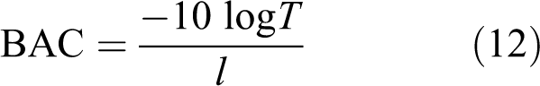
where l is the optical path length (m) as determined by the particular instrument used for the measurement.
VI. Turbidity measurement units, calibration methods and standards
1. A summary of the major turbidity standards
The following three standards are in common use throughout the sub-disciplines of water quality assessment. Although other standards do exist, these three are the most commonly cited by researchers into the properties of natural waters. The summaries of these standards are presented in order to highlight some of the technical imprecision inherent in their measurement methodologies.
US EPA method 180.1
This standard has been in use in various revisions since the early 1970s. The most recent revision being 2.0 (US EPA, 1993), which states that it is applicable to the measurement of turbidity in ‘drinking, ground, surface, and saline waters, domestic and industrial wastes’ (US EPA, 1993, p.1). The standard employs the comparison between the light scattered by the test sample to the light scattered by a ‘standard reference suspension’ (US EPA 1993, p.1). This reference suspension consists of a defined mixture of two chemicals, hydrazine sulphate and hexamethylenetetramine, to produce a ‘stock standard suspension’ known as formazin (US EPA, 1993, p.3). A primary standard suspension is then created by diluting 10 ml of stock standard in 100 ml of reagent water. This concentration is defined as having a turbidity of 40 nephelometric turbidity units (NTU). Another acceptable commercially available primary standard based on styrene divinylbenzene polymer is also stated.
The instrumentation parameters for the measurement of scattered light by this standard are the use of a tungsten light source with a colour temperature from 2200–3000 K, and a beam path-length of not greater than 0.1 m. The detector response should peak at 400–600 nm, and the measurement angle should be 90° ± 30°. Note that this is a very broad range of light wavelengths and scattering angles which encompass forward-, side- and back-scattering geometries.
ISO 7027
This standard has been in effect in Europe since 1994. It relies in part on the use of light scattering and attenuation by standard suspensions for comparison with the same measurements in a test sample, as with EPA Method 180.1. A notable difference between the two standards is that ISO 7027 (1999) dictates the use of near infrared light (λ = 860 nm) for all measurements. The standard suggests that at wavelengths greater than 800 nm the interferences caused by natural colouration of the water (e.g. by dissolved humic substances) can be significantly reduced, an effect which has been observed by Hongve and Akesson (1998).
In addition to the measurement of diffuse radiation (i.e. nephelometry) expressed in formazin nephelometric units (FNU – in the range 0–40), the standard also defines a method for the ‘measurement of the attenuation of a radiant flux, more applicable to highly turbid waters (for example waste or polluted waters)’ (ISO, 1999). This measurement is expressed in formazin attenuation units (FAU), in the range 40–4000 FAU.
GLI method 2
This method is explicitly for the determination of turbidity in drinking water. It is a nephelometric and attenuation-based ratio-metric method based on infrared light of 860 nm wavelength, in common with ISO 7027. The use of dual-beam instruments that have two light sources and two detectors is specified. Each light source is pulsed sequentially, and for each measurement phase a 90° active intensity and a 0° reference intensity measurement is acquired (Figure 6). A ratio-based algorithm is then used to calculate an NTU value based on the four data points (i.e. two 0° and two 90° measurements). The accepted reason for employing this method is that it improves instrument stability due to interferences caused by the degradation of the light source, the fouling of sensor windows, and the effects of water colouration. It must be noted that the ratio algorithm is not defined in the standard, which implies that the implementation is left to the instrument designer (the topic of ratio methods is considered in greater detail later). As in the previously discussed standards, formazin suspensions are used for calibration. This is an example of a multiple parameter measurement method.
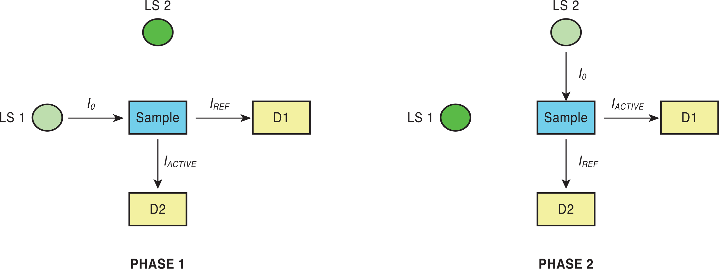
Beam-ratio process as described in GLI Method 2. LS 1 & LS 2 are the light sources; D1 and D2 are the detectors. I 0 is the light beam incident on the sample; I ACTIVE is the 90° scattered light and is considered to be the actual nephelometric measurement; I REF is the 0° transmitted light and is used purely as a reference value for use in a ratio-metric calculation.
2. A summary of turbidity measurement units
The US Geological Survey has summarized currently used turbidity units and their associated standards as reproduced in Table 2 (USGS, 2013), with amendments for the scattering angle convention in use throughout this paper.
Units of measurement for turbidity sensors, after USGS website (USGS, 2013).
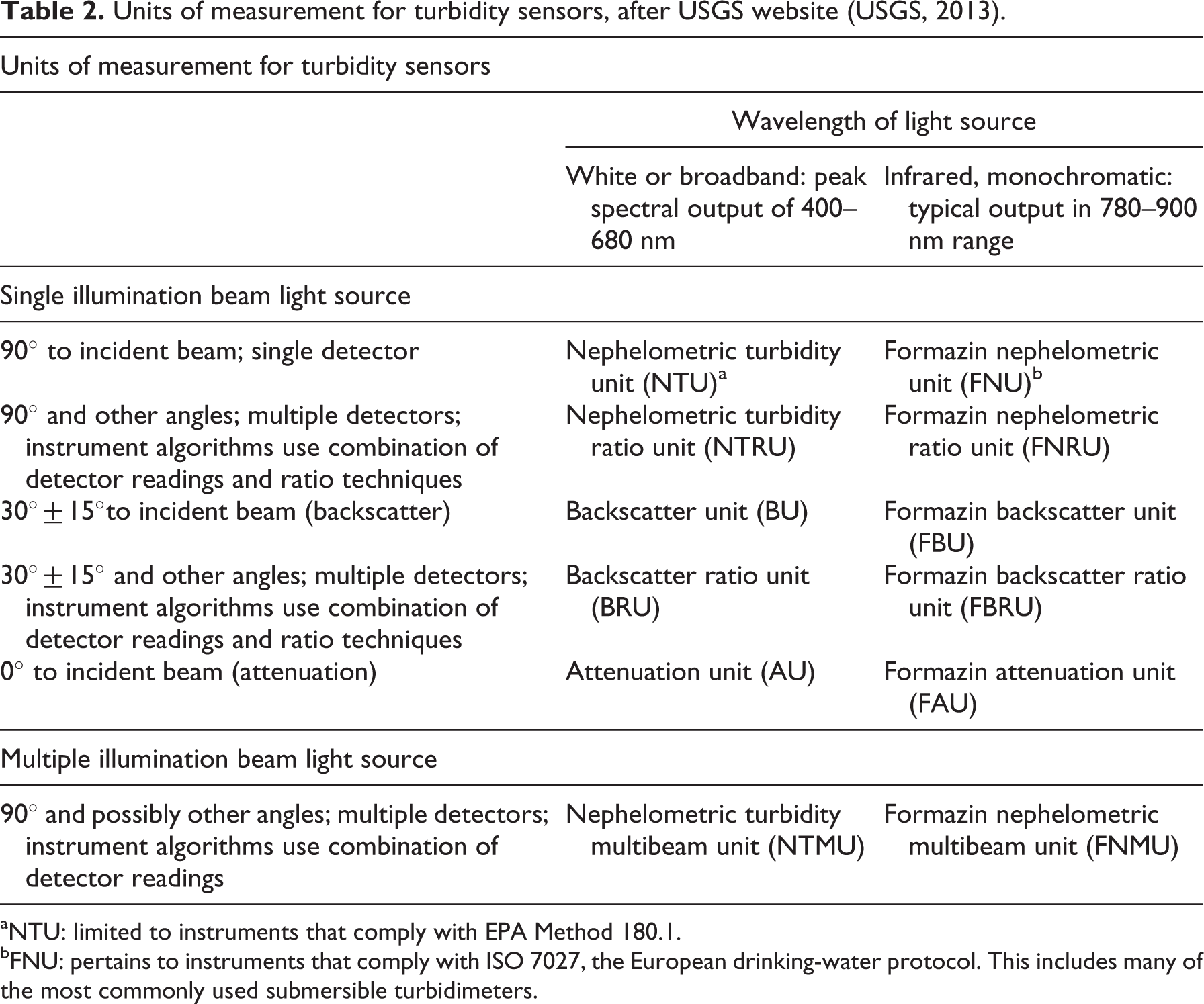
aNTU: limited to instruments that comply with EPA Method 180.1. bFNU: pertains to instruments that comply with ISO 7027, the European drinking-water protocol. This includes many of the most commonly used submersible turbidimeters.
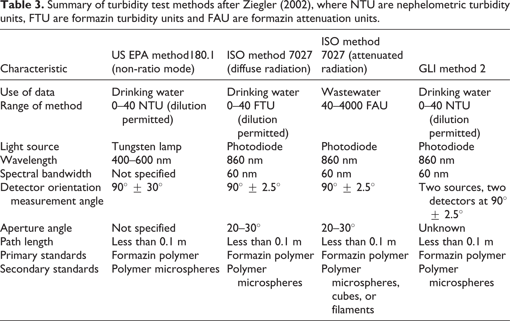
Most of the material reviewed for this paper pertains to measurements taken by turbidity instruments that comply with either USEPA Method 180.1 or ISO 7027, and hence the measurement units that are most commonly encountered in the literature are NTU, FNU (specifically for drinking-water assessment) and FAU (specifically for waste-water assessment). The USGS considers these units to be the ones that are most commonly applied to submersible turbidimeters. The other units listed in Table 2 are rarely encountered in the turbidity literature. In addition to the USGS website, another useful summary containing greater detail regarding the applications of the different turbidimeter designs is presented by Sadar (2004). A more concise summary of the standards discussed in this paper is presented by (Ziegler, 2002), and this summary is reproduced here (Table 3) as it provides pertinent and useful aid to the context of this discussion.
Summary of turbidity test methods after Ziegler (2002), where NTU are nephelometric turbidity units, FTU are formazin turbidity units and FAU are formazin attenuation units.
3. The problem with formazin
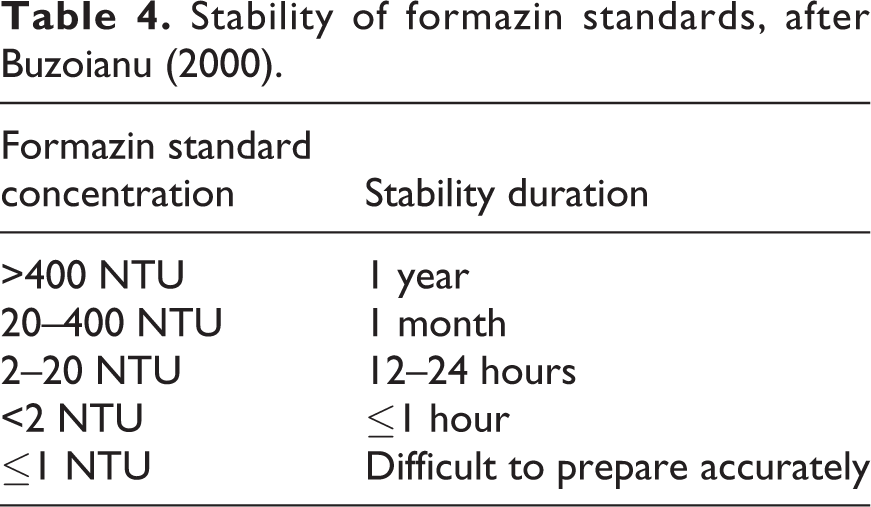
Formazin is useful as a turbidity standard as it can be reproducibly prepared from raw materials to within ±1%, and comprises a wide range of particle shapes and sizes ranging from 0.1 µm to 10 µm (Buzoianu, 2000). However, it also has a number of drawbacks as highlighted by Buzoianu (2000): The preparation temperature affects the resulting PSD. Formazin is carcinogenic. Formazin primary standards do not usually state the concentration uncertainty. The stability of formazin standards decreases as the concentration decreases (Table 4). The dilution ratio can be very high which leads to high uncertainty at low concentrations. This necessitates the use of secondary standards with longer shelf lives, and these standards can have poor repeatability of preparation, they are not formazin (e.g. latex), and they have different (narrow) PSDs. Hence, the use of secondary standards produces more variation in the response of different measurement instruments to the same nominal turbidity level.
Stability of formazin standards, after Buzoianu (2000).
It is a key fact that all of the units described in the previous section (Tables 2 and 3) are derived from a chemical concentration level of formazin or a secondary polymer-based standard. By this methodology an increase in concentration is defined as an increase in turbidity. There is no defined relationship between the stated turbidity and the measured light intensity. The word ‘concentration’ has effectively been replaced by ‘turbidity’ in the definition of these measurement units. For example, Section 7.3 of US EPA Method 180.1 states ‘Primary calibration standards: Mix and dilute 10.00 ml of stock standard suspension (Section 7.2) to 100 ml with reagent water.
This definition is a serious issue as ‘turbidity’ in these standard techniques no longer refers to an optical property of water, but rather a chemical concentration of what is in terms of particle classification an unknown distribution of both particle sizes and particle shapes. As the PSD is not known, it is therefore not repeatable between measurements due to factors such as chemical degradation and flocculation during storage of the ‘stock standards’. Also, the fact that it is deemed acceptable to use secondary standards that will not have the exact same optical response as formazin (Rice et al., 1997, p.110) suggests a flaw in the methodology at its root, as these ‘stock standards’ are clearly not consistent nor are they traceable.
The sphericity of the suspended formazin particles is also not quantified. Sadar (1999) states when describing formazin ‘the polymer in solution consists of random shapes and sizes’. Both PSD (Baker and Lavelle, 1984; Ziegler, 2002) and sphericity (Gibbs, 1978) have been shown to have a significant effect on the light-scattering characteristics of a suspension. Referring back to Figure 1, the dimensionless size parameter x has a large effect on the scattering phase function. For example, nephelometric instruments are most sensitive to particles of <1 µm diameter as in this size-range there is a significant amount of side-scattering, yet the standards do not state the PSD limits required for reference solutions.
It has been demonstrated that different instruments measure different turbidity values when calibrated with the same primary standard, due to the differences in instrument design (Buzoianu, 2000). This is a situation that can occur even when the different instruments are made to comply with the same measurement standard (e.g. EPA Method 180.1), due to the wide design tolerances (e.g. a measurement angle of 90° ± 30°). In view of the large uncertainties in the concentrations (and PSDs) of the calibration standards, augmented by the variation in measurement instrument response, there is then a scenario in which one stock standard and two different measurement instruments (made to the same or different standards) could potentially give rise to not two, but multiple different initial calibration results (Figure 7). An inaccurate surrogate model of turbidity has now effectively become synonymous with turbidity itself by definition in these standards. This calibration problem has implications for the measurement of turbidity in the field. The cross-comparability of measurements made by different researchers at different sites using different instrumentation is now questionable, even if each researcher has a self-consistent set of repeatable calibration data for their own particular measurement instrument. It is therefore necessary to take a step back and to re-define the chain of measurement at its first and weakest link, which is the formazin standard, and to establish a new methodology based purely on the calibration of measurement instruments to well-defined light intensities at well-defined wavelengths.
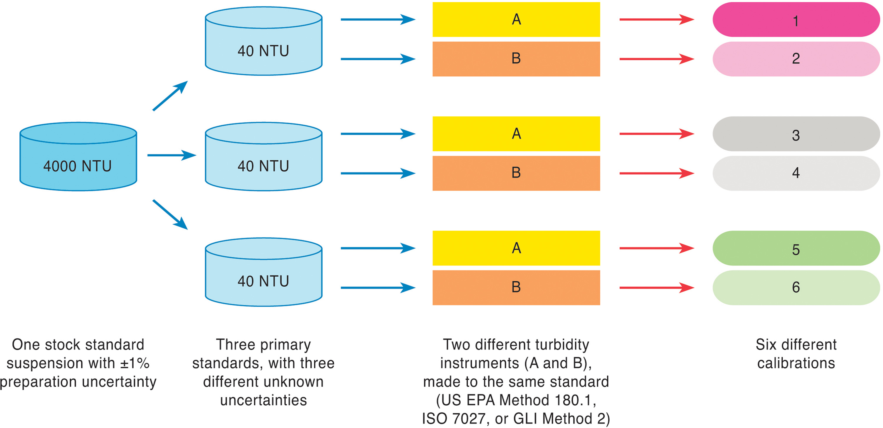
An example of the effect of indeterminate PSD due to identically defined but potentially physically dissimilar primary turbidity standards on the calibration of turbidity instruments. Results are further confounded by the variability in response between different instruments to the same PSD.
VII. Towards a new turbidity instrumentation standard
In order to move towards a new standard for the design of turbidity instrumentation it is first necessary to take a step back from the accepted suspension-based calibration methods as prescribed by the existing standards. The following discussion attempts to clarify the misconceptions associated with the relationship between SSC, TSS and turbidity, and leads on to a proposed calibration methodology based on the measurement of light-attenuation due to the presence of optical neutral density (ND) filters in the optical beam path. To complete the new standard, a new nomenclature based on the BAC is proposed for the reporting of turbidity at multiple scattering angles and wavelengths of light. To conclude the discussion, some suggestions for the contents of potential secondary standards (based on the newly proposed instrumentation standard) for surrogate SSC determination are then outlined briefly.
1. SSC and TSS: their relationship with turbidity and the importance of the PSD
The surrogacy of physical properties for intrinsic optical properties as is the case regarding chemical concentration becoming a surrogate for optical turbidity has raised the possibility of further misinterpretation, due to the undefined PSD of the calibration standards and the inconsistent response of different measurement instruments to the same PSD (Buzoianu, 2000). In this section it is necessary to take a step back from turbidity to examine the meanings of the pre-existing terminology for suspensions (of sediment or otherwise) in water. It is important to understand this terminology as the descriptive acronyms actually refer to documented test methods for the determination of sediment concentration and suspended solids concentration. An understanding of these methods will then facilitate a deeper appreciation of the reasons for the conceptual conflation of sediment concentration with turbidity.
The US convention regarding the attribution of documented test methods to the acronyms ‘SSC’ and ‘TSS’ has been adopted in this paper. Regarding this terminology, as with that of turbidity, the differences in use in different disciplinary areas arises again. For example, Holliday et al. (2003) suggest TSS to mean ‘total suspended sediment concentration’, rather than ‘total suspended solids’, i.e. the acronym SSC may have been a better choice.
The field techniques and laboratory methods for the measurement of SSC and TSS were reviewed by Gray et al. (2000), who cite Method D 3977-97 (ASTM, 1998) for SSC and Method 2540 D (APHA, 1971) for TSS. They describe the two different analytical methods as follows: SSC data are produced by measuring the dry weight of all the sediment from a known volume of a water-sediment mixture. TSS data are produced by several methods, most of which entail measuring the dry weight of sediment from a known volume of a subsample of the original.
After an analysis of 3235 paired SSC and TSS measurements was performed, it was concluded that SSC was the more reliable methodology (Gray et al., 2000), especially when the amount of sand in a sample exceeds approximately one quarter of the dry sediment mass. The main reason given for this disparity of results is that the SSC analytical method utilizes the entire sample (including all sediment present), whereas the TSS methods typically involve the analysis of only a sub-sampled aliquot of the total sample. The decanting and pipetting techniques employed to obtain this aliquot do not capture a complete representation of the sediment population of the original sample. The resulting sub-sample is therefore sediment deficient, particularly of the larger sand-sized sediment fraction. Gray et al. (2000) go on to suggest that the reason for this loss of sediment during TSS analysis arises from the fact that TSS methods were originally designed for analysis of waste-water samples that were to be collected after an initial settling phase, hence larger sediment particles were never intended to be part of the analysis. They finally conclude that SSC and TSS analysis of natural water samples are not comparable, and that SSC is the only viable method for the determination of the sediment concentration of natural waters.
In order to relate a subjective turbidity reading to a real physical property such as SSC, a calibration procedure is typically performed. This relationship between the optical properties of suspended sediment and its mass concentration must therefore be understood, requiring the characterization of its lithology. The size of the sediment particle is frequently measured either directly (e.g. filtering and sieving), or analytically (by laser diffraction) in the case of smaller size fractions. Laser-based particle size measurements give a volume concentration value, which then requires further knowledge of the specific density and mineralogy of the sample in order for an estimate of the mass concentration to be obtained. This process is known as end-member calibration.
The problem now arises that the detector response has been pre-calibrated to a primary standard, with arbitrary units for turbidity based on unstable calibration methods. It has already been suggested (Figure 7) that these units (NTU, etc.) are not comparable between calibrations made on instruments constructed to the same standard. It is therefore highly unlikely that calibrations made by different instruments (constructed to the same or different standards) can ever be accurately compared due to the invalidity of these extrinsic turbidity units. It is therefore necessary to determine the true instrument response by a different method entirely. Only then can an end-member calibration have any chance of being meaningful.
Optical ND filters are regularly employed for the calibration of transmission-based optical instruments, but are seldom employed in turbidimetry or nephelometry. These filters provide a consistent optical density (OD) which in turn will attenuate a well-defined percentage of the transmitted light. One such example of an attempt to calibrate a turbidimeter against a known light attenuator is that by Finlayson (1985). By not only calibrating a turbidimeter against Formazin suspension, but also against ND filters, Finlayson has devised a method by which direct comparison between attenuation measurements made on the same sample by different devices could potentially be developed. It can be seen that Formazin concentration does not in fact have a linear relationship to measured light attenuation (Figure 8). Although the calibration data are sparse in the upper range of the instrument in this case (Finlayson, 1985), there is a good fit of the data to a power law (R2 = 0.9954). The only two useful axes on this graph are ‘meter reading’ and ‘neutral density filters’, as these two alone are all that is required to accurately establish the response of the instrument to attenuation (Figure 9). Only when this detector attenuation curve has been established can further selective end-member calibrations be performed to determine the effect the PSD has on the response of a particular instrument to a given sediment. Each ND filter represents an optical density, d, which is directly equivalent to the absorbance A, as in equation (4). So in order to calculate the BAC in dB m−1 for an instrument with path-length l, the following equation can be applied:
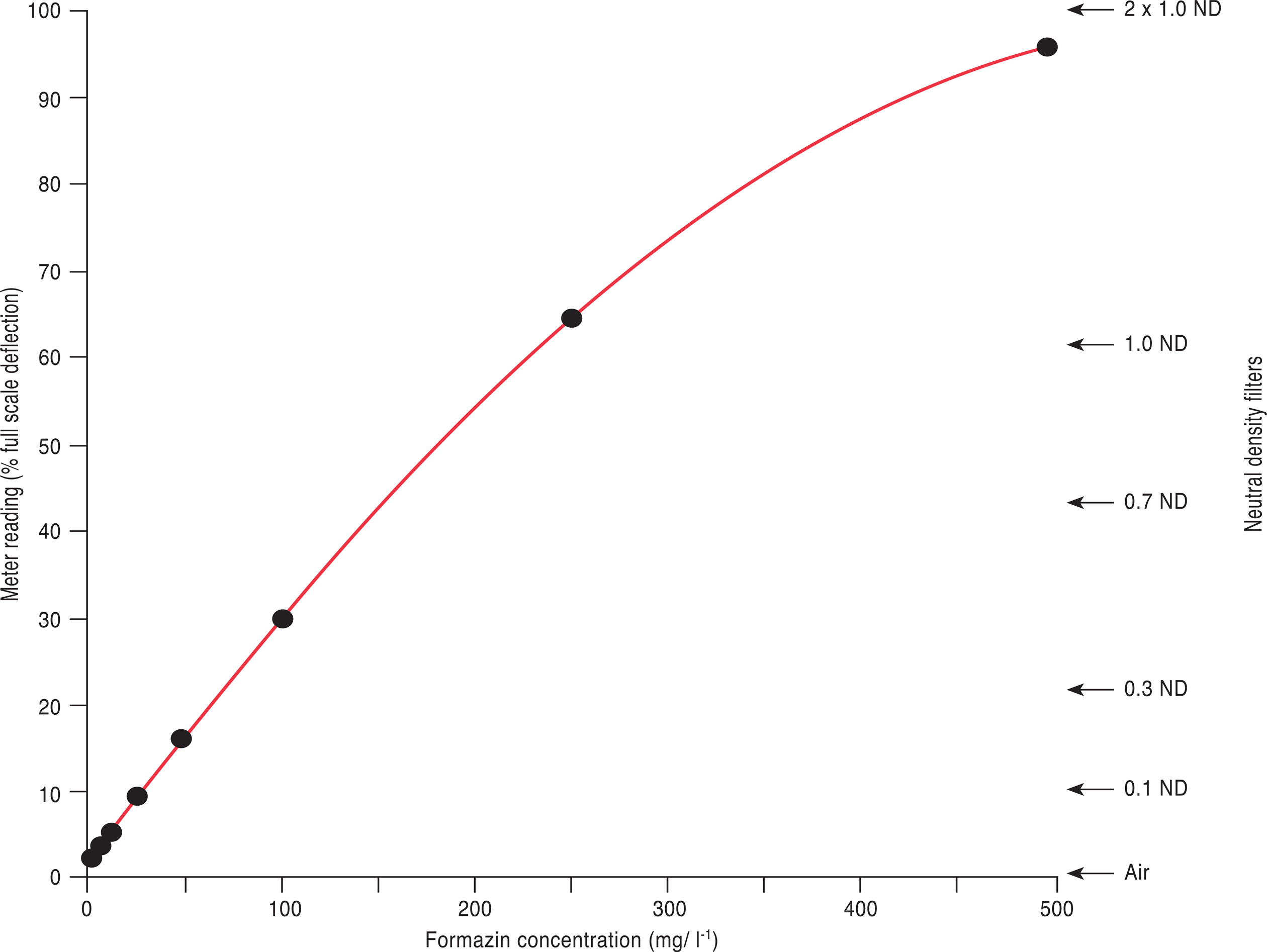
Laboratory calibration of a turbidity meter with formazin standards. Meter readings of the neutral density filters used in the field are shown also (Finlayson, 1985).
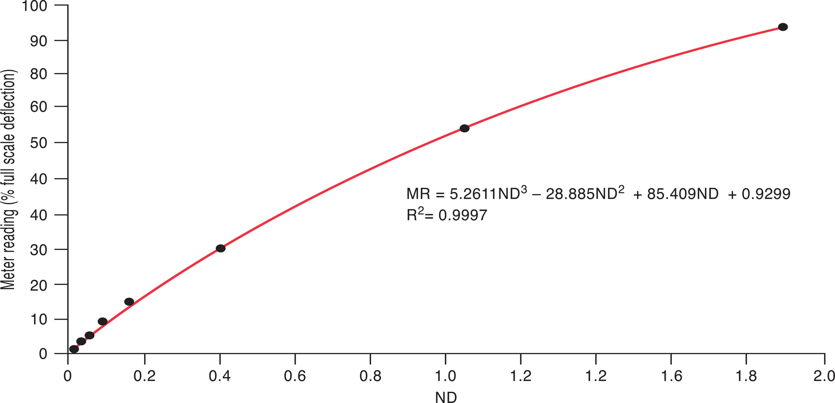
A reproduction of the data contained in Figure 8 showing the meter reading vs. the ND filter value (after Finlayson, 1985). The ND value is equivalent to d, the optical density.
2. Instrumentation parameters and calibration methods
To arrive at a consistent methodology for the measurement of turbidity it is necessary to accept that the only quantity that can be readily measured optically in this context is the transmitted light intensity, and hence attenuation with respect to the light source (i.e. I/I 0). It is the methodology for taking this measurement that should be rigorously specified, regardless of the measurement angle θ with respect to I 0. The implementation section of the standard should address this methodology, and focus purely on the desired response of the instrument to light at defined intensities and wavelengths. This aspect of work would involve the definition of parameters such as sensor type, variable intensity light source specification (including coherence and polarization), detector amplifier gains and ranges, ND filter calibration procedure involving multiple beam paths, beam path-length and collimation arrangements. It is then necessary to decide which instrument parameters (e.g. θ, λ and l) should be specified as mandatory for all turbidity measuring instruments, and which ones should be considered as being application-specific.
VIII. The reporting of turbidity measurement data
The standardization of the reporting of turbidity as attenuation data (Ziegler, 2002) and the use of a more descriptive nomenclature is proposed, which will allow for the easy identification of application-specific data such that incompatible measurements will not be inadvertently compared to each other. It is suggested that significant progress could be made if the measurement concepts for turbidimetry and nephelometry were unified, i.e. by treating them both as an attenuation process. The only difference being that for scattered light measurement the effective concentration of scatterers is inversely proportional to the BAC measured at a specific angle to the incident beam. However, for that to be achieved formulations of the BAC at specific angles must then be defined, for example BAC0 for a standard transmissivity measurement and BAC90 for the nephelometric counterpart at 90°. For the nephelometric case the relationship between the scattered light intensity and the concentration could be viewed as an inverse attenuation, since a higher concentration of particles will produce stronger scattering (until the concentration is too high, at which point multiple-scattering and grain-shielding will dominate and interfere with the measurement of the side-scattered light). Measurement-instrument calibration now becomes somewhat critical, as any drift in the incident light intensity or the sensor response will affect the sensitivity of the system to the low light intensities that need to be detected due to side- or back-scattering. This nephelometric BAC90 measurement results in potentially larger percentage errors than those that are likely for measurements based on BAC0, as greater electronic amplification is required to detect the weaker scattered-light signal which can be inherently noisy. In order to formulate a generic equation for the BAC as a function of measurement angle it is necessary to include two terms: one for attenuation and one for scattering. The use of these terms is in no way a new idea (e.g. Kirk, 1985); however, the interpretation of scattered light intensity as an inverse absorbance has not been previously considered. In this new method the same measurement units could be employed for practical comparison between data obtained under different conditions using different instruments, so long as those instruments complied with the same instrumentation standard, and the reporting of said data is consistent (Ziegler, 2002). For example, Kirk (1985) suggested using the correct description of the measurement method, such as ‘side-scattering’, when stating results – or preferably BAC90 in this case.
IX. Standards for surrogate SSC determination
Further standards for the determination of surrogate properties such as SSC should refer to instruments that are specified according to the new instrumentation standard. In order to estimate SSC accurately, optical instruments must be capable of producing data rich enough to facilitate suspended sediment characterization. Methods for the determination of the PSD (and other properties) of a suspended sediment by multi-parameter measurements need to be developed, which could include the use of laser diffraction techniques. Other potential methods of sediment characterization should also be explored more thoroughly.
1. Suspended sediment characterization
For a deeper understanding of sediment transport to be realized, it is essential to know how the different size classes of sediment respond to different flow conditions, especially the larger sand-sized particles that can be transiently in suspension long enough to affect turbidity measurements. A knowledge of sediment particle shape in terms of sphericity and roundness can also provide an insight into the distance travelled by sediment particles that have previously been entrained in a flow of water. There is a clear need therefore to characterize the suspended sediment to determine the particle sizes present. This characterization can be achieved by traditional gravimetric sampling methods, but there is an increasing need to gather data for research purposes in-situ and quickly. In some cases, these measurements could be made ‘off-line’ by optical means, which would still be much faster than can be achieved by gravimetric methods. Laser-based optical measurements are the most commonly employed for this purpose, although there have been attempts to derive particle-size information from multi-parameter turbidity measurements. The effect that particle shape has on such measurements could also be exploited as a characterization technique.
2. Measurement ratios and multi-parameter method development
The designers of some turbidity meters (i.e. any commercially available instrument that claims compliance with GLI Method 2) have adopted the use of multi-parameter measurements in order to improve instrument performance. This innovation has included the measurement of light intensities at multiple scattering angles, and the use of the ratios of those intensities to infer some of the physical properties of the scattering suspension, e.g. sphericity (Gibbs, 1978), or to negate the effect of water colour as an interference to the turbidity measurement (Lambrou et al., 2009; Lawler, 1995). An example of another multi-parameter approach to turbidity measurement is presented by Yang and Hogg (1979), wherein two different wavelengths of light are used to predict the PSD of the scattering suspension. These and other multi-parameter approaches to turbidity measurement should be the focus of further research, and will aid the development of new turbidity standards.
X. Conclusions
The use of turbidity purely as an indicator of water clarity is entirely acceptable assuming the development of more consistent standards. The problem is that the existing standards have introduced a set of measurement units that actually represent a surrogate for turbidity and therefore cannot be used to describe water clarity.
Simple turbidity measurements when used as a surrogate for SSC are only viable under highly constrained conditions. Bias toward the fine sediment fraction is usually considered unimportant, but this is not always the case.
Sand-sized sediment fractions are not consistently accounted for by existing turbidity measurements, due to their high settling velocities. The SSC method is also required in order to quantify the sand fraction fully.
The development of new light-scattering models will permit more sophisticated approaches to turbidity measurement, in particular by the use of parameter-rich data sets obtainable from multi-parameter methods. This approach will facilitate the improvement of turbidity standards, and could increase the accuracy of large sediment particle detection.
A new turbidity instrumentation standard needs to be drafted, based purely on the principle of attenuation for calibration and reporting purposes. It should specify the reporting of the BAC in dB m−1 (or derived units) for a range of measurement angles and wavelengths of light. This standard should be a root standard from which other secondary standards are derived, e.g. standards for suspended sediment characterization or TSS assessment by optical turbidity measurement.
A further standard for suspended sediment determination by simple multi-parameter turbidity measurements needs to be devised (leading on from point 4 above). This standard should include basic sediment characterization as an outcome of optical turbidity measurements (e.g. PSD and sphericity).
Footnotes
Declaration of Conflicting Interests
The authors declared no potential conflicts of interest with respect to the research, authorship, and/or publication of this article.
Funding
The authors received no financial support for the research, authorship, and/or publication of this article.