A review of spatial statistical approaches to modeling water quality

Abstract

We review different regression models related to water quality that incorporate spatial aspects in their model. Spatial aspects refer to the location of different sites and are usually characterized by the distance between different points and directions by which they are related to each other. We focus on spatial lag and error, spatial eigenvector-based, geographically weighted regression, and spatial-stream-network-based models. We evaluated different studies using these methods based on how they dealt with clustering (spatial autocorrelation) of response variables, incorporated those clustering in the error (residual spatial autocorrelation), used multi-scale processes, and improved the model performance. The water-quality-based regression modeling approaches are shifting from straight-line distance-based spatial relations to upstream–downstream relations. Calculation of spatial autocorrelation and residual spatial autocorrelation was dependent upon the type of spatial regression used. The weights matrix is used as available in the software and most of the studies did not attempt to modify it. Different scale processes like certain distance from rivers versus consideration of entire watersheds are dealt with separately in most of the studies. Generally, the capacity of the predictor variables to predict the response variable significantly improves when spatial regressions are used. We identify new research directions in terms of spatial considerations, weights matrix construction, inclusion of multi-scale processes, and identification of predictor variables in such models.

Keywords

Water quality hydrology watershed spatial statistics spatial autocorrelation scale

I Introduction

Water quality, defined as the physical, chemical, and biological characteristics of water, is directly associated with human and ecosystem health. Water quality itself is dependent on various factors, including land cover, land use, land management, atmospheric deposition, geology and soil type, climate, topography, and catchment hydrology (Lintern et al., 2018). Water-quality parameters vary across space and time as a consequence of variations in these different factors. For effective water-quality management, it is crucial to understand these factors and the pathways by which they affect water quality. Understanding the spatial patterns of water-quality parameters and factors affecting them, therefore, is crucial in pinpointing locations of interventions for improving water quality in surface water bodies.

The most common approach of water-quality research involves the statistical method, which typically process raw quantitative data using mathematical models, formula, and techniques to extract information and generate meaningful output (Nature Statistics, 2019). Regressions are the most common statistical methods to understanding the relationship between water quality and watershed characteristics (Chang, 2008; Shi et al., 2016; Zhou et al., 2012). Regression approaches may or may not include spatial aspects of water-quality parameters (Ullah et al., 2018). Spatial aspects refer to location and relative position to each other, usually analyzed using spatial statistical methods. A relatively new sets of spatial statistical approaches, which typically extend from linear regression analysis, attempt to incorporate spatial processes to identify environmental and spatial determinants of water quality in surface water (Blanchet et al., 2008; Legendre, 1993).

Many studies have examined spatial aspects of water quality (e.g. spatial autocorrelation and distribution of high and low values along a river network) using various modeling techniques to explore the effect of landscape-level variables in the water quality. These studies include several review papers that synthesized different aspects of water-quality research. Giri and Qiu (2016) reviewed the current understanding of the relationship between land use and water quality, while Ullah et al. (2018) examined different statistical approaches to modeling water quality using land-use types as predictor variables. Lintern et al. (2018) conducted a comprehensive review of key factors affecting the spatial patterns of water quality, while Guo et al. (2019) reviewed various factors affecting temporal patterns of water quality. Isaak et al. (2014) conducted a review of research on a group of spatial statistics, spatial-stream network (SSN)-based models. However, there is not any comprehensive review related to the spatial aspects of water-quality modeling that offers water-quality researchers a way to understand the basic concept of the spatial statistics and help them choose an appropriate modeling approach.

We carry out this review to compare different statistical models based on their effectiveness in addressing spatial aspects of water quality. We specifically examine spatial autocorrelation of the water-quality parameters, residual spatial autocorrelation (RSAC), use of weights matrix, and incorporation of directional spatial processes in the model. First, we discuss how these methodologies have evolved, and later we perform a systematic literature review to identify knowledge gaps related to spatial autocorrelation, the use of multi-scale processes, and directional spatial processes. We review papers related to spatial lag and error model, spatial eigenvector-based models, geographically weighted regression (GWR), and SSN-based models. We recognize that there are other spatial modeling approaches that are not covered in this review, including spatial kriging, P-splines, and several spatial autoregressive models (e.g. McLean et al., 2019).

II Spatial statistical approaches in water-quality studies

In watershed science, watershed, basin, or sub-basin are considered units of analysis. Extracting predictor variables that affect surface water quality mostly involves consideration of the entire watershed. Several ways exist to incorporate different scales in the water-quality modeling endeavor (Allan, 2004; Mainali and Chang, 2018). One of the most common involves creating a buffer of a specified distance from stream or lakes. Some studies also use a threshold distance upstream from the sampling point (e.g. Shi et al., 2017). Some new methods provide higher weight to the landscape factors close by the streams based on Euclidean (straight line) distance, flow distance, or flow accumulation (Grabowski et al., 2016; King et al., 2005; Peterson et al., 2011).

Spatial variations in the watershed properties draining into the river result in variable water quality across different parts of the river, which typically lead to a specific spatial pattern of water quality. As nearby places are more alike than distant spaces (Tobler, 1970), there might be a cluster of high or low values of water-quality parameters. This phenomenon, spatial autocorrelation, is a measure of whether a data value of one location is independent of the data values of other locations (Sokal and Oden, 1978). Spatial autocorrelation can be positive when similar data values are close to each other, or negative when dissimilar data values are neighbored (Legendre, 1993; Sokal and Oden, 1978). Spatial autocorrelation opens new avenues to statistically analyze seemingly obvious but ignored spatial patterns of water quality and their relations with the watershed attributes (Legendre, 1993).

A family of statistical tools is being used to analyze spatial autocorrelation among sampling stations. Moran’s I is the most commonly used measure to evaluate the pattern of the attributes as clustered, dispersed, or random in space. This is a global statistics, one that offers a single set of statistics for the entire set of data. Moran’s I has been used to analyze different water-quality attributes in order to identify whether the water-quality attributes show any global pattern of spatial dependence (Liu et al., 2016; Miralha and Kim, 2018; Pratt and Chang, 2012). As Moran’s I statistics only offer information about the level of spatial autocorrelation for an entire set of data, we cannot use it to identify any local clusters. There are a few statistical approaches developed to identify local clusters in spatial data and they are also being used to explore clusters of sites with degraded or not-degraded water quality. Getis–Ord’s G_i and local Moran’s I are commonly used in such local statistics (Anselin, 1995; Getis and Ord, 1992). These methods identify whether or not similar high or low values are clustered together locally and identify those clusters in geographical space. Many water-quality-analysis works have used these statistics to explore local relations in a sampling space (Brody et al., 2005; Mainali and Chang, 2018; Tu and Xia, 2008).

The spatial autocorrelation in any data is associated with spatial dependence among neighboring data points, resulting in a spatially biased trend and violating the assumption of independence of most standard parametric statistical procedures (Cliff and Ord, 1972; Legendre, 1993; Sokal and Oden, 1978). In regression analysis, biases due to such neighboring data points need to be accounted for, as they can produce autocorrelated residuals (differences between actual and predicted values) and ultimately inflate Type I error, leading to wrongfully rejecting the null hypothesis (Bini et al., 2009; Cliff and Ord, 1972; Miralha and Kim, 2018). It is not possible to account for such influence only using traditional simple linear regression approaches that assume that data points are randomly distributed in the sampling space, and that model residuals are not autocorrelated. Several spatial regression approaches that account for such spatial dependence are being used in water-quality modeling, including spatial lag model, spatial error model, GWR, spatial eigenvector mapping, and SSN-based models (Blanchet et al., 2008; Borcard and Legendre, 2002; Brunsdon et al., 1998; Getis and Griffith, 2002; Ver Hoef and Peterson, 2010; Ver Hoef et al., 2018).

III Spatial weights matrix and spatial regression models in water-quality studies

1 Spatial weights matrix

The spatial dependence between sampling points is formally expressed as a weights matrix and is a necessary element of spatial regression models (Anselin, 2001; Getis and Aldstadt, 2004). Each spatial weight refers to the relative influence of different spatial units under consideration to the candidate spatial unit. These weights matrices can be defined in several ways, according to spatial interactions among different factors under consideration, and the hypotheses of interest (Sokal and Oden, 1978). The most essential aspect of the weights matrix is defining a neighborhood set for each location. The neighborhood sets are specified for each location as the row and the neighbors as the columns in a matrix. Non-zero weight is assigned when observations are within a given number of nearest neighbors or a specified distance. In the spatial statistics literature, the weight can be specified based on Euclidean distance, economic distance, number of nearest neighbors, or empirical flow matrices (Anselin, 2001). The weights matrices use several approaches to incorporate the effect of adjacent observations. Sometimes, a certain number of nearest neighbors is used, while in other cases only observations within a certain distance are used, with the same weight to all the observations within that distance (Figure 1). Spatial regression models usually differ in terms of conceptualizing the spatial relationships, usually through the weights matrix. In this section, we discuss how these different spatial regression approaches are conceptualized and used in water-quality modeling endeavors (Figure 2).

Figure 1.

Conceptualization of different weights matrices. 1) Spatial contiguity: a spatial weights matrix is created based on whether polygons share a common boundary or not (a binary decision with 0 or 1). For example, for P1, four polygons (i.e. P2, P3, P6, P8, and P9) are considered as neighbors based on Queen’s connectivity), or P6 will not be included if a zero-distance common boundary (i.e. point connectivity) does not count (Rook’s connectivity). A contiguity-based spatial weights matrix can be specified with either the length of a common boundary or the area of an adjacent polygon instead of 0–1 binary values. For example, for the length of a common boundary, P9 has the longest common boundary with P1 and, thus, will have the largest weight, while P8 shares the shortest common boundary with PI and has the smallest weight. For the area of an adjacent polygon, P3 is the largest adjacent polygon of P1 and will have the largest weight, while P2, which is the smallest adjacent polygon of P1, has the smallest weight. 2) Nearest neighbor: sometimes weight can also be provided based on the numbers of neighbors for each candidate polygon (k-nearest neighbor). If we only use one closest neighbor, polygons (first order) defined in the Queen’s case (P2, P3, P6, P8, and P9) are considered. If two nearest neighbors (second order) are considered, in addition to the polygons adjacent to P1, the polygons sharing a boundary with those (P2, P3, P6, P8, and P9) are also included during the weights matrix construction for the candidate polygon (P1), which results in the inclusion of P4, P7, and P10, but not P5. Nearest neighbors (which are often called k-nearest neighbors) are specified with a fixed number of neighbors. It is often adoptively utilized for a case in which observations are not (relatively) evenly distributed. For example, one remote point (it is often specified for points) may not have any neighbor, which is a problem in spatial analysis. To avoid this problem, k-nearest neighbors can be utilized. 3) Threshold distance: spatial neighbors can be specified based on a preset distance from the centroid of a polygon. Here, with a threshold distance d1, polygons inside the circle of radius d1 are considered as spatial neighbors for polygon P1. In this case, P1 has four neighbors: P2, P3, P8, and P9. If d2 is used for a threshold distance, all polygons but P4 and P5 are neighbors of P1 and have a non-zero weight.

Figure 2.

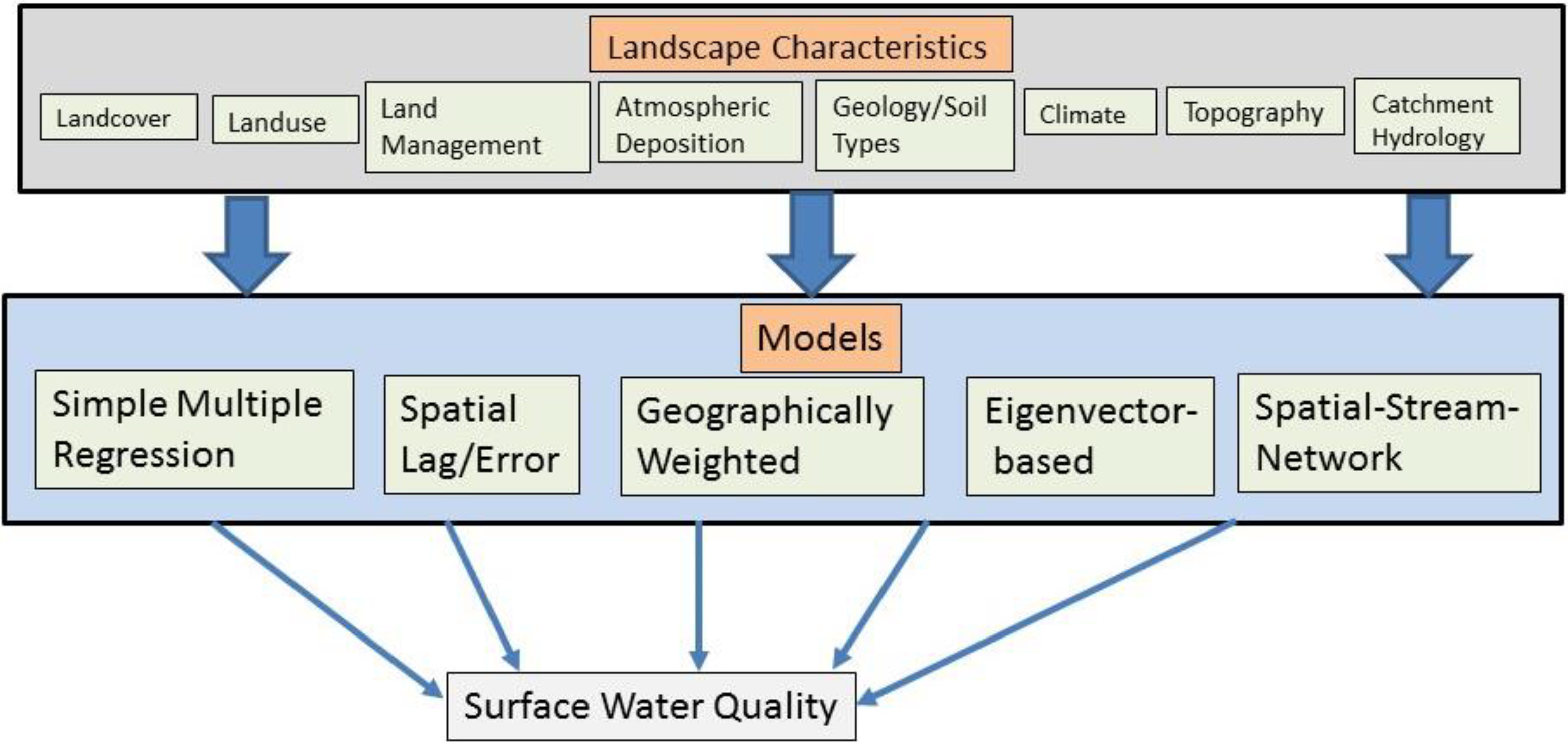
Use of different landscape characteristics (Lintern et al., 2018) in different spatial statistical modeling approaches considered in this review.

2 Spatial lag and error model

Spatial lag models and spatial error models are the most commonly used global regression models that account for spatial dependence among observations in a model specification. Global models refer to the regression models that produce a single set of model parameters for a set of data. A spatial lag model (Anselin, 1988, 2001) is applied when response variables suffer from significant spatial autocorrelation. A spatially lagged variable is created by averaging the values of the response variable at neighboring locations (Figure 3). The spatial lag model includes a spatially lagged dependent variable with a weights matrix to account for the spatial autocorrelation. Such a weights matrix is often constructed without consideration of a stream network, so it tends to have more neighboring sites than that of a stream network (Figure 3(a)). A spatial error model (Anselin, 2001) is used when model residuals suffer from significant spatial autocorrelation. This is similar to the spatial lag model except that it accounts for spatial autocorrelation in the error term.

Figure 3.

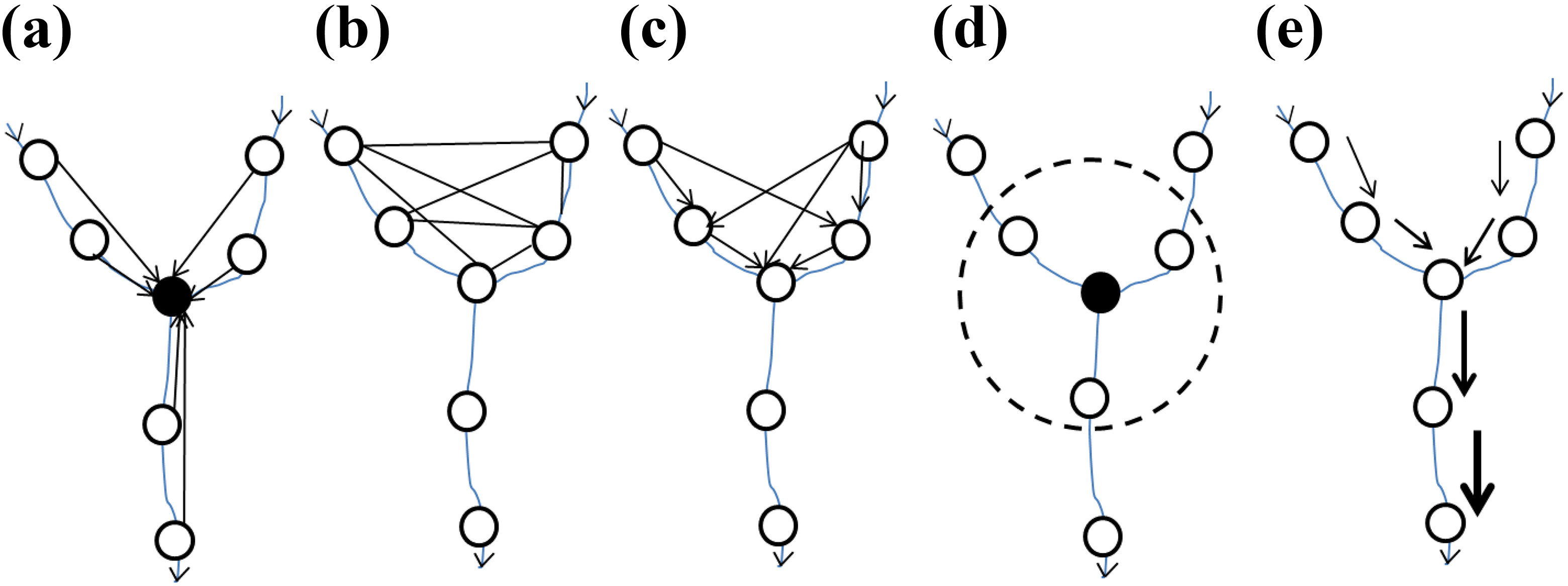
Spatial relations among sampling stations for a spatial weights matrix creation in different types of spatial modeling for surface water quality. The black arrows refer to directionality of the spatial relations and the dotted circle represents a certain bandwidth. (a) Both upstream and downstream stations affect a station of interest. (b) All surrounding stations are considered with no directionality between upstream and downstream stations (modified from Sharma et al., 2011). (c) Asymmetrical configuration: only upstream stations are considered, but stations in different tributaries could affect each other. (d) Only neighbors within a threshold distance are considered with no specific upstream and downstream relationships. (e) SSN model: arrows in SSN models refer to the direction of the relation and moving average function; the width of the arrow refers to the strength of the influence for each potential neighborhood location; spatial autocorrelation occurs when the moving average function overlaps (modified from Peterson and Hoef, 2010).

Several researchers have been using these methods to model water quality and reported a general improvement in model performance when such spatial models are used (Chang, 2008; Huang et al., 2016; Miralha and Kim, 2018). This improvement in the model performance typically relates to the degree of spatial autocorrelation and RSAC (Kim and Shin, 2016; Kim et al., 2016; Miralha and Kim, 2018).

3 GWR

Global spatial regression models, such as spatial lag models and spatial error models, are used to develop a spatially rectified global regression model by accounting for the spatial dependence of an entire dataset. They only produce a single set of statistics for the entire dataset under consideration. Therefore, they are a member of global spatial regression models. In reality, a relationship between predictors and a response variable can vary within a catchment, and the strength of those relations might also be different across regions. In order to address this issue, GWR can be used to allow model coefficients to vary for each observation and create a set of local models based on the location of sampling sites (Brunsdon et al., 1998). The observed data included in each local model are geographically weighted, depending on the proximity of the location, and are used to estimate local R ² and coefficients for each sample observation. The number of samples included for each data point is defined using a bandwidth function (e.g. Figure 3(d)). Although a fixed-distance band can also be used, a flexible bandwidth that adapts to the spatial pattern of the data can be more effective, particularly when data are not evenly distributed over space (Fotheringham et al., 2002). During the modelling process, the nearby data points are weighted more heavily than those from more remote locations using a kernel function. GWR is increasingly used in water-quality modeling, not only to estimate the model parameters but also to explore the variabilities of those relationships in different watersheds (Chen et al., 2016; Chang and Psaris 2013; Pratt and Chang, 2012; Tu, 2011).

4 Moran’s eigenvector maps and spatial filtering

Eigenvector-based models are spatial models in which the vectors are derived using neighborhood criteria or distance with neighbors. In these models a matrix can be constructed based on the geographical distance between locations. This matrix is transformed into eigenvectors by eigenfunction decomposition (e.g. Figure 3(b)). This method was originally proposed by Borcard and Legendre (2002) as the principal component of neighborhood matrix, also called Moran’s eigenvector maps (MEMs). This method incorporates spatial autocorrelation in modeling ecological processes. Eigenvectors corresponding to positive eigenvalues are used as spatial descriptors in regression or canonical analysis (Borcard and Legendre, 2002). Vrebos et al. (2017) modeled the water quality of 75 stations in the Kleine Nete catchment in northern Belgium and reported that about 30% of variation was explained by catchment land cover while about 11% was explained by spatial eigenvectors created from Moran's Eigenvector Maps.

There are both distance-based eigenvector maps and spatial filtering based upon a geographic connectivity matrix (Borcard and Legendre, 2002; Getis and Griffith, 2002; Griffith, 2010; Griffith and Peres-Neto, 2006). Eigenvector-based spatial filtering is used to separate spatial effects in regression modeling from model residuals so that a standard regression model can be used without suffering from spatial autocorrelation (Getis and Griffith, 2002). Similar to the eigenvector mapping approach, it also uses “eigenfunctions of spatial configuration matrices to derive the spatial eigenvectors” (Griffith and Peres-Neto, 2006). This approach has been used to model soil attributes (Kim et al., 2016), plant diversity (Kim and Shin, 2016), crime patterns (Chun, 2014), and diseases (Jacob et al., 2008). Mainali and Chang (2018) used this approach to model the water-quality trends of the Han River Basin, South Korea, reporting that it significantly increased model performance and removed the RSAC.

5 Asymmetrical eigenvector maps (AEMs)

All of the spatial statistical approaches discussed in the previous section assume that the relations among sampling sites are multi-directional. The spatial associations of different points along the river are usually unidirectional as the water flows downstream (e.g. Figure 3(c)). Therefore, upstream water quality affects downstream water quality but not vice versa. Recently, new spatial statistical methods have been developed in order to account for such directionality in water-quality modeling. Blanchet et al. (2008) modified the MEM approach in order to incorporate the directional process of rivers and streams as AEMs. They propose that “gradients influencing spatial distribution can be studied via spatial variables (eigenfunctions) that represent directional spatial processes”. This is also a part of the eigenfunctions-based spatial filtering framework, with the added feature that it “constructs space in an asymmetric way” by only accounting for the sites connected through the water flow. The modeling involves defining a connection diagram based on the directional spatial process and creation of sites-by-edges matrix, which are transformed into spatial eigenvectors.

6 Spatial-stream network (SSN)

A river can be effectively represented as a dendritic network, and any scientific inquiries and management decisions related to river networks should acknowledge this (Peterson et al., 2013). Dendritic networks use points and lines in geographical space, and typically have a directional component (Peterson et al., 2013). The modification of the autocovariance model that incorporates the dendritic network structure of rivers is dubbed a SSN model (Ver Hoef et al., 2006, 2014). It uses a set of autoregressive functions to derive the predictor variables to be used in the regression modeling. The weight of those directional processes can be river distance, flow volume, or catchment size, or any relevant variables for the watershed of interest (e.g. Figure 3(e)). The SSN allows users to test spatial autocorrelation and develop models for various scenarios like flow-connected, flow-unconnected, and Euclidean distance (Isaak et al., 2017; Neill et al., 2018; Scown et al., 2017). It not only allows the development of models but also lets users explore the spatial properties of the data in relation to various in-stream processes (e.g. McGuire et al., 2014).

IV A systematic review of current studies

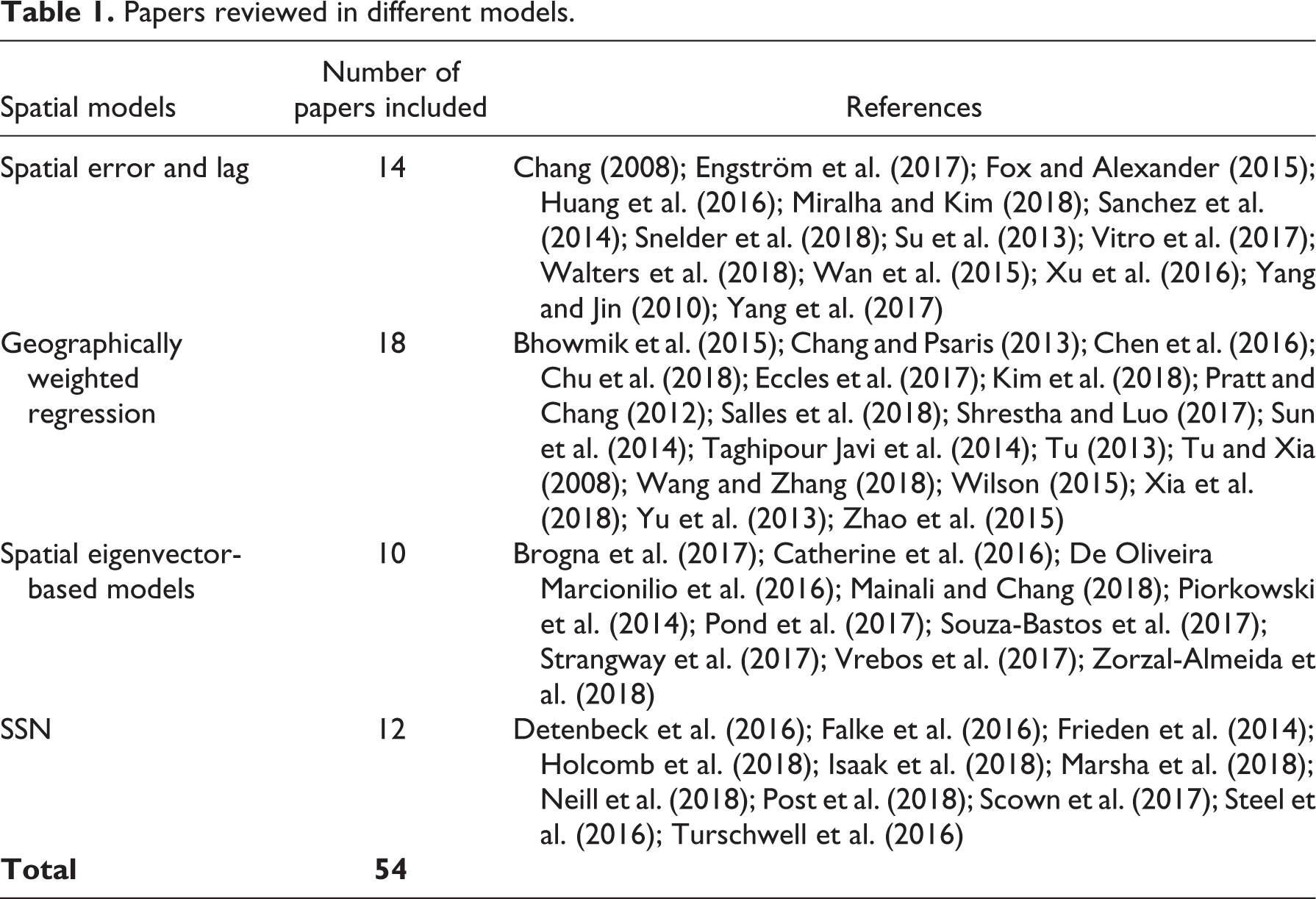
We carried out a systematic review of articles related to different types of spatial regression of water quality published from 2000 to 2018, using the Web of Science database on November 9, 2018 (Table 1). The search phrases we used included “water quality” and “spatial regression”, “water quality” and “eigenvector”, “water quality and “autocorrelation”, and “water quality” and “spatial-stream network”. We identified 54 articles with a water-quality focus that used at least one type of spatial regression (Table 1). Note that it may not be a comprehensive list, as we only searched for the term “water quality”. The water-quality information might well be published as water pollution, or in terms of individual parameter names such as temperature, pH, nitrogen, or phosphorus. These names were not included in our search terms. We also removed studies that did not have spatial regression approaches. Although we mostly focused on surface water, we also included a few groundwater-quality works in this review. We focused our review on the use of spatial statistical methods to account for spatial autocorrelation and RSAC, weights matrix construction, scale considerations, and improvements in model performance in different types of spatial statistical modeling. We also attempted to identify the spatial pattern of these studies to explore where such research efforts have been concentrated.

Table 1.

Papers reviewed in different models.

Spatial models	Number of papers included	References
Spatial error and lag	14	Chang (2008); Engström et al. (2017); Fox and Alexander (2015); Huang et al. (2016); Miralha and Kim (2018); Sanchez et al. (2014); Snelder et al. (2018); Su et al. (2013); Vitro et al. (2017); Walters et al. (2018); Wan et al. (2015); Xu et al. (2016); Yang and Jin (2010); Yang et al. (2017)
Geographically weighted regression	18	Bhowmik et al. (2015); Chang and Psaris (2013); Chen et al. (2016); Chu et al. (2018); Eccles et al. (2017); Kim et al. (2018); Pratt and Chang (2012); Salles et al. (2018); Shrestha and Luo (2017); Sun et al. (2014); Taghipour Javi et al. (2014); Tu (2013); Tu and Xia (2008); Wang and Zhang (2018); Wilson (2015); Xia et al. (2018); Yu et al. (2013); Zhao et al. (2015)
Spatial eigenvector-based models	10	Brogna et al. (2017); Catherine et al. (2016); De Oliveira Marcionilio et al. (2016); Mainali and Chang (2018); Piorkowski et al. (2014); Pond et al. (2017); Souza-Bastos et al. (2017); Strangway et al. (2017); Vrebos et al. (2017); Zorzal-Almeida et al. (2018)
SSN	12	Detenbeck et al. (2016); Falke et al. (2016); Frieden et al. (2014); Holcomb et al. (2018); Isaak et al. (2018); Marsha et al. (2018); Neill et al. (2018); Post et al. (2018); Scown et al. (2017); Steel et al. (2016); Turschwell et al. (2016)
Total	54

1 Geographic distribution of studies

The majority of study sites of research related to spatial statistical modeling of water quality are concentrated in the USA and China, with a few exceptions: Canada, Brazil, South Korea, Australia, and some countries in Europe (Figure 4). This is likely because of the fact that these countries have relatively dense networks of monitoring stations over a large area. Only 15 nations were represented from 54 studies. Although developing countries are most vulnerable to water-quality degradation (Schwarzenbach et al., 2010), very little research has been carried out there. This list may not be comprehensive, but we assume that this map represents the spatial pattern of current research related to spatial aspects of water quality.

Figure 4.

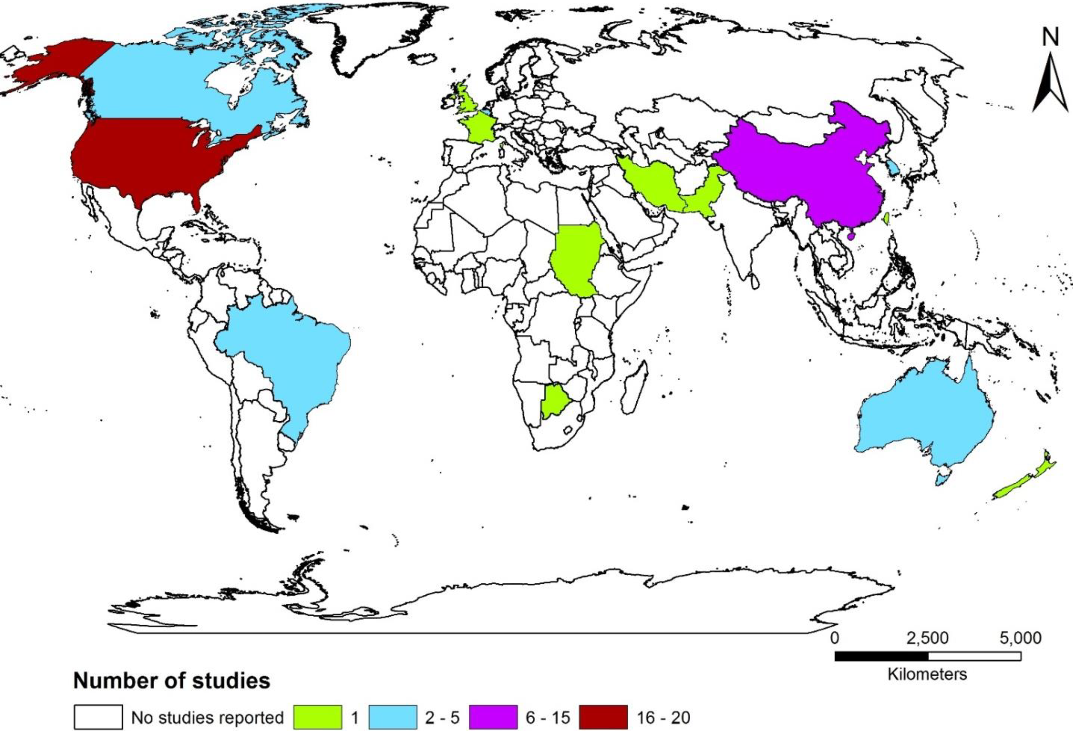
Country-wise distribution of the sites of the studies included in this review (n = 54).

2 Spatial autocorrelation in different spatial regressions

Theoretically, exploring the spatial autocorrelations of the dependent variables and residual autocorrelations, and examining the significance of spatial autocorrelations, are the first steps in incorporating spatial relations into the models. Although the relationship between RSAC and variation of the model (pseudo-) R ² and coefficients is discussed in most of the studies, the relationship with the spatial autocorrelation of dependent variables is usually not taken into consideration. Many latest studies have reported that the spatial autocorrelation of dependent variables and RSAC are usually related; the choice of covariates also affects the significance of RSAC (Mainali and Chang, 2018; Miralha and Kim, 2018).

We find that the use of spatial autocorrelation statistics of the dependent variable is generally associated with the type of spatial regressions used. Approximately 43% of papers that used either a spatial lag model or a spatial error model calculated the spatial autocorrelation of the dependent variable, while only 30% of papers using an eigenvector-based model did so. Similarly, 43% of papers using GWR calculated the spatial autocorrelation of the dependent variable, while about 75% of Spatial Stream Network Model (SSNM) papers did so. Forty eight percent of spatial-error/lag papers, 70% of eigenvector-based papers, 61% of GWR papers, and 100% of SSN model papers tested for RSAC.

The analysis of spatial autocorrelation in water quality leads to a better understanding of the extent of spatial organization (clustered, dispersed, or random) of water-quality variables, and also helps explore the capacity of the independent variables to predict the water-quality pattern (e.g. Miralha and Kim, 2018). Accounting for spatial autocorrelation in regression can correct bias in parameter estimation and, hence, helps avoid an incorrect conclusion for potential factors. A higher percentage of RSAC testing in more recent studies stems from the fact that the independent variables might not explain all the spatial autocorrelation and results in RSAC – that is, it is the spatial autocorrelation in residuals that should be examined. A high level of spatial autocorrelation in the response variable may give a hint for spatial autocorrelation in residuals, but is not necessarily a reason to use spatial regression as long as there is no significant RSAC. A future research suggestion in this field would be checking for RSAC before using spatial regression models if the researchers are concerned that the regression model does not account for the spatial autocorrelation.

3 Spatial weights matrix

All spatial statistical modeling approaches are based on some form of spatial weights matrix. The most common type of weights matrix – distance matrix – is constructed using the distance among the sampling sites based on geographical coordinates; sites are weighted based on distance, number of neighbors, or other relevant attributes. The other attributes include Euclidean distance upstream, river distance upstream, catchment size, and river flow (Isaak et al., 2018). There are several standard distance matrices available for different types of spatial regression approaches. For example, spatial lag and spatial error methods use nearest-neighboring stations (Chang, 2008; Huang et al., 2014); the spatial filtering approach uses at least one neighbor; the geographically weighted approach mostly uses adaptive bandwidth to include the desired number of sites; and SSN uses river distance, flow volume, or upstream catchment area. However, spatial statisticians recommend modifying the weights matrix based on the hypothesis being tested, the scale of analysis, the spatial distribution of the sampling station, and spatial issues being addressed (Blanchet et al., 2008; Sokal and Oden, 1978).

Based on our review, we find that most of the papers use a “standard” weights matrix provided by the software on which the model is being implemented. Traditionally, spatial lag models use observations in all directions to create a spatial lag variable. Some studies attempted to modify the existing weights matrix to incorporate hydrologic connectivity. For example, Vitro et al. (2017) modified a spatial weights matrix to incorporate the effect of only upstream stations in a spatial lag model. They provided relative weights to upstream stations based on the proximity to the candidate station being considered. Engström et al. (2017) used two different weights matrices, one with all proximate stations and the other with proximate and upstream stations. Most other studies used only a set number of nearby stations to define weights. For example, Chang (2008) and Huang et al. (2014) used four closest stations, Su et al. (2013) used 10 such stations, and Yang and Jin (2010) used only adjacent stations. However, no study has tested how the study results might be sensitive to changes in weights matrices.

GWR uses an exponential (or Gaussian) distance decay function to create spatial weights among the sampling sites included within the specified distance defined by the bandwidth. A majority of the GWR papers use flexible (or adaptive) bandwidth to derive the spatial weights to be used in the regression models. An adaptive bandwidth allows the band (or buffer) around a sampling station to vary according to the number of nearby sampling stations. The bandwidth is small for clustered data and large for scattered data, based on the distance between sampling stations. Most of these papers use a software-defined standard bandwidth approach (mostly adaptive bandwidth) available in ArcGIS. We did not find any studies that use GWR by including the effect of only upstream stations. However, Tu (2013) used sampling stations only from mutually exclusive watersheds, thereby avoiding any complexity that would be caused by upstream stations in the model. While this approach avoids the issue of upstream influence on downstream water quality, the sample size will be lowered as many spatially dependent stations are discarded for analysis. Additionally, most studies did not address the potential issues of a small sample size when GWR models were used for water-quality studies. This can be a new research direction where researchers define the band only towards the upstream stations and weight those values to derive the local models, which, hypothetically, would better explain the local patterns. Our hypothesis is based on the general understanding of the river flow where most of the physical and chemical components flow downstream.

The research papers using MEM and AEM approaches also use a standard weights matrix based on the Borcard and Legendre (2002) method. As scale can be an issue in these kinds of weights matrices, some researchers construct eigenvectors at different scales. For instance, De Oliveira Marcionilio et al. (2016) calculated their weights matrix using eight different distance classes (50–450 m, with an interval of 50 m) to incorporate the effect of scale on their analysis. The SSN modeling approach was initially proposed to incorporate weights based on the stream distance, flow volume, or stream order. When flow volumes are not available, the catchment area is commonly used as a weight attribute (Ver Hoef and Peterson, 2010), but other attributes such as slope, Shreve’s stream order, and Euclidean distance among stations are also used depending upon the nature of the watershed and the availability of data.

We notice from this review that a spatial weights matrix typically does not gain enough attention, in spite of its being the backbone of spatial modeling. Most previous studies rely on a weights matrix readily available in the “standard” tools offered in software packages, rather than putting additional effort into generating a revised weights matrix that considers water flow along the hydrologic network. Therefore, researchers ought to be mindful of the spatial relations of water quality in the sampling space, and design the weights matrix to best capture such spatial relations. We also need to be aware of the spatial relations of water-quality sampling sites to source, mobilization process, delivery mechanism, and in-stream movement, and use appropriate weighting schemes to capture those processes.

4 Use of multi-scale processes

The predictor variables for regression analysis are generally derived using a watershed because all of the water flowing in the river comes from some part of the watershed, and watershed characteristics are reflected in river water quality (Allan, 2004). Researchers have worked to identify the scale at which water quality is best correlated with watershed characteristics (Figure 5). Although a majority of researchers used spatial lag/error, GWR, or MEM to extract predictor variables at different scales, they did not compare the effect of different scales in model prediction (Table 2). They rarely used different scaled data under the same regression model. The papers using SSN models, however, recognized the effects of variables at different scales and incorporated those in the models.

Figure 5.

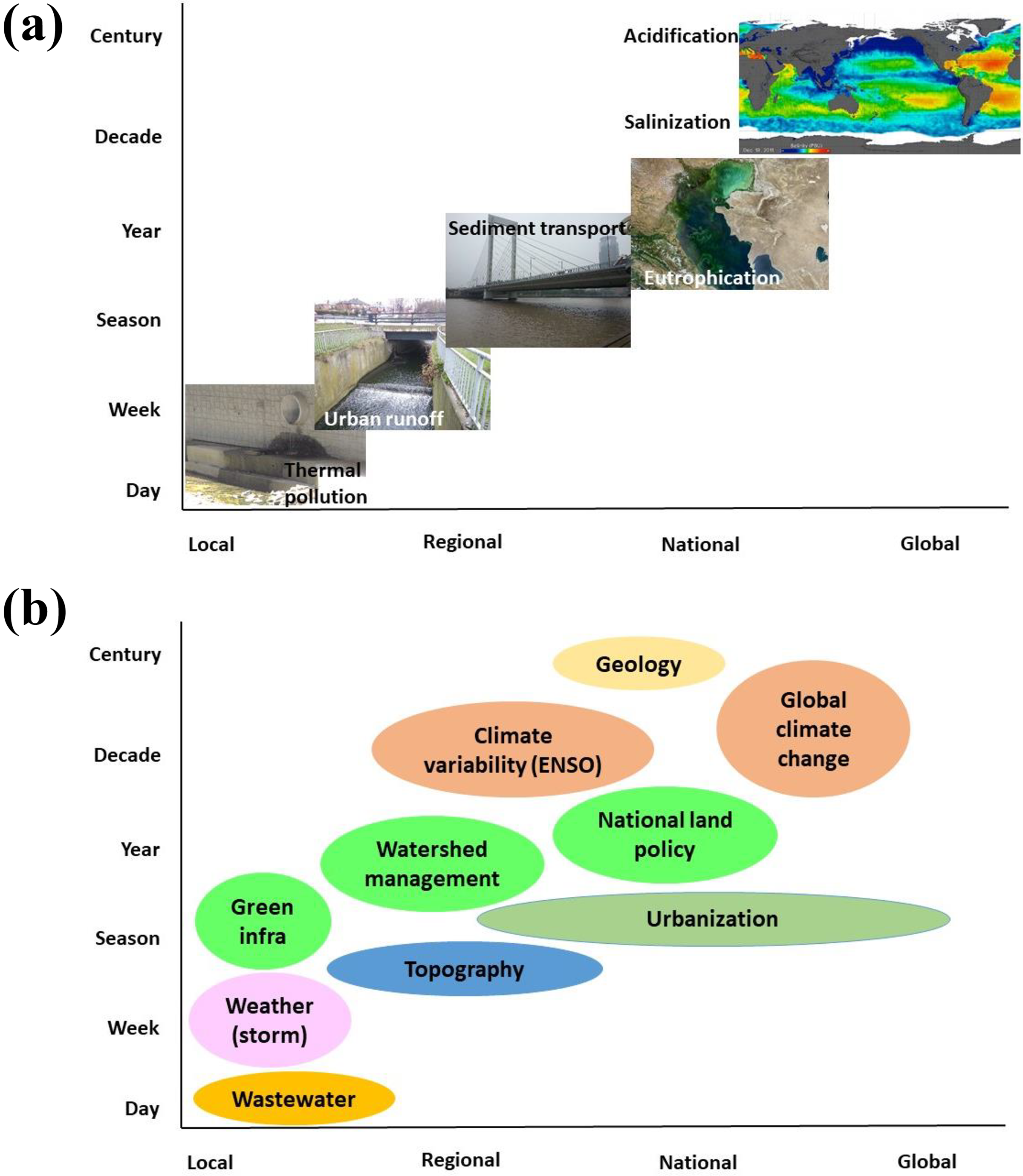
(a) Scale-dependent water-quality processes; (b) factors affecting water quality at different space and time scales.

Table 2.

Consideration of weights matrix, spatial autocorrelation, and residual spatial autocorrelation.

Model type	Scale	Spatial autocorrelation (SAC)	Weights matrix	Residual spatial autocorrelation (RSAC)
Spatial lag/spatial error	Predictor variables extracted at multiple scales. Entire catchments (Yang and Jin, 2010), a buffer of a certain distance (Chang, 2008), circular upstream buffer, multi-scale (Chang, 2008; Su et al., 2013).	About 60% of the papers evaluate the SAC of the response variable before pursuing these models.	Most of the papers use a weights matrix based on the Euclidean distance between neighboring stations, while some modify it to test a different hypothesis (e.g. Engström et al., 2017; Vitro et al., 2017).	Most of the papers do not evaluate whether RSAC has been an issue or not. Only a couple of papers used it (Engström et al., 2017; Miralha and Kim, 2018).
Eigenvector-based (MEM/AEM/spatial filters)	Some papers only used the watershed while the majority used different scales (Mainali and Chang, 2018; Strangway et al., 2017). Scale information derived from eigenvectors is also used (Vrebos et al., 2017).	Only about a quarter of papers that appeared in our list explored global or local SAC.	Most papers used a standard weights matrix derived using a binary coded sites-by-edges table and distance between the sites. Some modify it based on the distance classes (De Oliveira Marcionilio et al., 2016).	The majority of papers report RSAC of the model, except Strangway et al. (2017). RSACs are removed when this modeling approach is used.
Geographically weighted regression (GWR)	Although the majority of papers only use the watershed or some distance from the sampling station, some of the papers used different scales (Pratt and Chang, 2012).	The autocorrelation of the response variable is tested scantly.	Mostly an adaptive- or fixed-bandwidth approach is used, as available in the software. Shrestha and Luo (2017) ensured that there are statistically large number of stations considered as neighbors for each station (119) nearest neighbors in each local models.	As there is an inbuilt function to test RSAC in the ArcGIS interface of GWR, most of the papers mention it in their model.
Spatial-stream network (SSN) model	Most of the papers using SSN use a multi-scale approach where relevant covariates are extracted from either the whole watershed, or buffer, or using distance-weighted approaches (Isaak et al., 2018; Turschwell et al., 2016).	Semivariograms and Torgegrams are used to explore SAC almost exclusively, although some papers do not discuss it explicitly.	Different attributes are used as weights, like river distance, discharge, and catchment size, with different spatial connectivity considerations, like flow connected, not connected, and Euclidean matrix.	The RSAC of the models is tested almost exclusively and SSN models have been found to remove it.

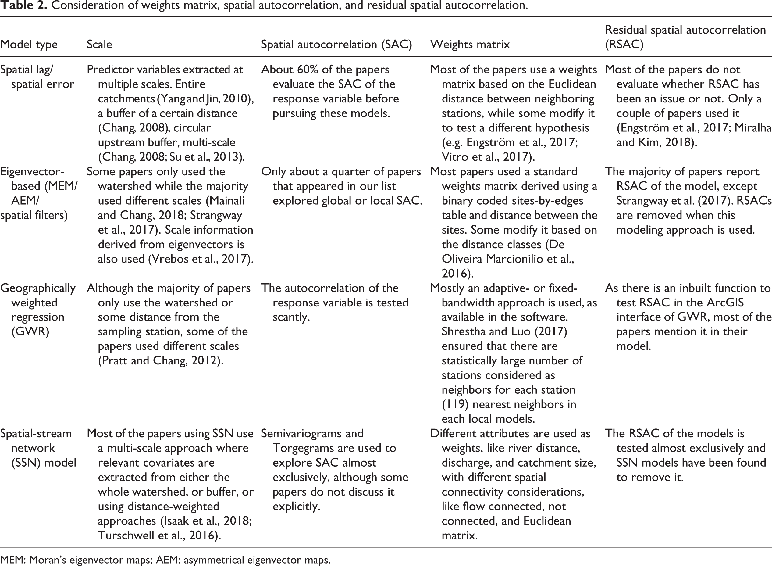
MEM: Moran’s eigenvector maps; AEM: asymmetrical eigenvector maps.

Some researchers have used different buffer distances from the river and/or sampling station. For example, vegetation cover within a 10 m buffer is used for temperature modeling by Isaak et al. (2018), while other variables were used at the watershed scale. Turschwell et al. (2016) used a 10 m buffer for riparian vegetation and additionally used inverse-distance-weighted effects of grazing land cover, while other variables were used as the lump attributes at the watershed scale, and reported significantly higher R ² values when SSN models were used.

Like any other natural processes, the factors affecting water quality operate at different scales. These factors have to be identified based on the understanding of the scale related to the source, mobilization, delivery, and instream processes related to these parameters (Lintern et al., 2018). This also depends on the scale at which disturbances drive water quality (Pond et al. 2017). If an “upland disturbance” is a driving factor of deteriorating water quality, using data derived only at the riparian buffer scale does not work (Pond et al., 2017). Our review also shows that the scale effects in water-quality modeling using landscape characteristics are not universal, as they vary by parameters studied, location, seasons, and covariates used (Liu et al., 2017; Mainali and Chang, 2018).

Isaak et al. (2018) argue that the covariates used in modeling approaches should come from a review of the literature and an understanding of a plausible mechanism that could cause a variation in a particular water-quality parameter. If the scale is not clear for the parameter, it is always safe to start with the watershed scale and incorporate other scales (e.g. Mainali and Chang, 2018). In large-scale analysis, the availability of particular datasets also determines the scale at which covariates are extracted. Our review shows that the researchers should be able to provide explanations for the reasons behind choosing a particular covariate, its scale, and the need for any weights treatment in the spatial statistical modeling of water quality.

Water flowing from various parts of a watershed drains into surface water bodies via multiple pathways. Water quality along the stream network, therefore, depends on the sources of the parameter, their delivery, and instream processes occurring in the vicinity of an area where water flows (Lintern et al., 2018). To best capture such spatial variations, researchers need to collect data or install the monitoring network carefully. The spatial and temporal scale of data collection and monitoring should be informed by the available geographical information of the watershed related to land use, human impact, geology, and hydrological characteristics of the stream. While increasing the spatial and temporal scale of analyses could help improve our understanding of the relationship between water quality and landscape variables, such effort requires time and resources (both human and computation resources). To make optimum use of time and resources, a selection of the data collection sites and appropriate scale should incorporate all the relevant characteristics of the range of watershed conditions (Jackson et al., 2015).

While it is beyond the scope of this paper to list all of the different scales at which predictor variables are extracted, here we list different statistical methods to effectively include different scale processes in water-quality modeling identified in the papers we reviewed. Multi-scale datasets can be treated with principal component analysis to reduce the dimension of the data and include the variability of different scale processes (Miralha and Kim, 2018). Redundancy analysis can identify which variables at what scale can explain variation in water quality, and use them as a predictor in the spatial regression (Strangway et al., 2017). To avoid overfitting the data that identify the best subset of the covariates, a “Best Subset Regression” can be used (Scown et al., 2017). The Best Subset Regression uses Akaike information criteria (AIC) variation to identify a maximum number of covariates set by the analyst. A review of the potential factors affecting water quality is of the utmost importance before undertaking any water-quality modeling efforts. From our review, we notice that there might be dozens of such candidate covariates. An appropriate variable reduction or selection method should be used in order to include a manageable number of water-quality parameters representing different scales.

5 Comparison of model performance

As expected, the spatial regression models typically explain the variation of the dependent variable better than their aspatial counterparts (Table 3). Studies using spatial lag and error models generally reported improved model performances from an aspatial linear regression model. An increase in R ² and a decrease in AIC indicate the improved model performance of these models over an aspatial one (Chang, 2008; Engström et al., 2017; Huang et al., 2014; Yang and Jin, 2010). While using an eigenvector-based spatial filtering approach, Mainali and Chang (2018) reported that the model strengths (R ²) significantly increase when an aspatial model suffered from RSAC. However, most of the eigenvector-based spatial statistical models we reviewed did not make an explicit comparison between aspatial and spatial models, as they used landscape characteristics and eigenvectors in the same model and used redundancy analysis to parse out the effect of “environmental” and “spatial” predictors (Souza-Bastos et al., 2017; Vrebos et al., 2017). GWR-based models consistently showed higher model strengths than linear regression. Chu et al. (2018) reported that GWR performed better than linear regression, which was superseded by geographically and temporally weighted regression. Similarly, Tu (2013) reported that the model performance increased by up to 10-fold when GWR was used against linear regression models. Tu and Xia (2008) also found some “dramatic” increases in R ² when GWR models were used. Most other papers using GWR for water-quality modeling also reported a significant increase in model performance (Kim et al., 2018; Pratt and Chang, 2012; Shrestha and Luo, 2017; Sun et al., 2014; Yu et al., 2013). The SSN-based models have shown to produce high R ² values in modeling water-quality parameters. An R ² value of higher than 0.9 was reported for modeling summer temperature using SSN (Isaak et al., 2018). Turschwell et al. (2016) found SSN performing strongest among different models used. However, in some cases, SSN-based models did not significantly improve model performance (e.g. Frieden et al., 2014). These varying results appear to be associated with the choice of water-quality parameters, landscape variables, the scale of analysis, sample size, and watershed conditions.

Table 3.

Improvement of model performance using spatial statistical models.

Source	Water-quality parameters	Predictor(s)	Change in model performance
Spatial lag and error model
(Yang et al., 2017)	TN	Land-use types and hydrological soil groups	Increases in R ² values ranged from 0.06 to 0.12
(Miralha and Kim, 2018)	pH, temp, SC, DO, TDS, TN, DIN, KjN, TP, tur, Br, Cl, Mg, Na, Ca, SiO₂, Fe, K, CO₂, Mn, Alk, SO₄, F, Csu, Chla, TOC, DOC, As, Cd, Zn, PO₄, NO₃, Al	Land cover, elevation, slope, hydrological soil groups	Increases in R ² values ranged from 0.03 to 0.29
(Vitro et al., 2017)	FC	Demographic, sewer lines, land cover, policy dummies	R ² values increased by 0.027
(Engström et al., 2017)	Microbiological contamination	Distance to informal settlement, share of informal settlement, different land use, distance to marshland	Reduction in model AIC from 158.31 to 153.2
(Sanchez et al., 2014)	Different components of biological integrity	Race, income, education, housing, population size, household size	DIC decreased in spatial model compared to non-spatial models (2131 vs 2064, 1848.7 vs 1673.8, 2428 vs 2270, 1252 vs 1143)
(Huang et al., 2014)	NH₄, NO₃, COD, SRP, Cl, Na, K, and Mg	Landscape composition, pattern, topography, geology, population, GDP	Increases in R ² ranged from 0.003 to 0.2
(Su et al., 2013)	DO, NH₃, and TP	Population, GDP, soil, land use	R ² values not compared. Only spatial regressions run
(Yang and Jin, 2010)	NO₃, NO₂	Land use/cover, soil, slope, area of watershed	Increase in R ² values ranged from 0.04 to 0.1
(Chang, 2008)	Temp, TN, TP, pH, COD, BOD, SS, DO	Land use, topography, soil	R ² values generally increased up to 0.3
(Fox and Alexander, 2015)	E. coli, TSS, DO, cond, temp	Land use, Floodplain, wildlife, elephant-specific fecal count, wildlife species	Quantitative change in R ² is not reported. But spatial models performed better
(Walters et al., 2018)	TP	Land-use composition and pattern, area, precipitation	Only results of spatial regressions reported
(Snelder et al., 2017)	TN, NO₃, TP, DRP	Climate, topography, geology, land cover	No comparisons were made
(Xu et al., 2016)	Nitrogen loss	Morphometric variables and soil drainage of each land-cover type	No comparisons, only spatial lag model was reported
Eigenvector-based models
(Souza-Bastos et al., 2017)	Hematocrit, plasma osmolality, sodium, Cl, Mg, K, cortisol, glucose	Different water-quality parameters	Spatial factors accounted for about 2% variation of dependent variables
(Wan et al., 2015)	Macroinvertebrates	Different water-quality parameters	Spatial factors (eigenvectors) more important than environmental factors. Overland distance worked better (6.7 to 9.5, and 10.2 to 10.7%)
(Brogna et al., 2017)	DO, DOC, TP, NH₄, NO₂, NO₃, pH, Cl, SO₄	Forest cover	Variability explained by forest covers when elevation is included accounts for 9.3% of variation in water quality, which would be 33.8 if elevation was not included
(Vrebos et al., 2017)	T, pH, O, NO₃, NO₂, NH₄, TP, CL, CO₂, BSi, Ca, Fe, K, Mg, Na, SiO₂, Zn, COD, SS, Chl-a, cond	Land use, soil	Space (Euclidean distance-based MEM) explained for both analyses circa 22% of variance. But none of the AEMs were significant predictors
(Strangway et al., 2017)	TP, OP, E. coli, KjN, DOC, pH, cond, various metals, NO₃, DO, Br, Ca, Mg, and SO₄, F, Hg, Sb, As, B, Se, Si, tellurium	Land use, road density	River-network-based model explained the greater variations than non-network-based model
(Catherine et al., 2016)	Phytoplankton species	Water-quality parameters, land use, rainfall, water temperature, and altitude	No significant effect of MEMs were reported in the model performance
(Mainali and Chang, 2018)	TN, TP, COD, SS	Land use, topography, soil, population	Increase in R ² ranged from –0.16 to 0.31
(De Oliveira Marcionilio et al., 2016)	Chl-a	Water-quality parameters, depth, vegetation cover	Addition of spatial factors as eigenvector slightly increased the model performance (39% vs 28%)
(Zorzal-Almeida et al., 2018)	Trans, CO₂, DO, cond, pH, NH₄, NO₃, TN, PO₄, TP, Chla, TOC, TN, TP, C/N, δ13C, δ15N	Land-use index	AEM R ²s are higher from 0.13 to 0.24 over MEM
(Piorkowski et al., 2013)	E. coli	Organic carbon, water velocity	MEMs explain 26.9% of the population variance during baseflow and 31.7% post stream flow
Geographically weighted regression (GWR)
(Xia et al., 2018)	Cu, Zn, Pb, Cr, and Cd	Land use	GWR didn’t always increase R ² values. R ² change ranged from –0.029 to 0.663
(Kim et al., 2018)	Cyanobacteria	Bands 2, 4, and 5 of Rapid Eye imagery	R ² increased to 0.719 from 0.615, AIC reduced from 1735 to 1710
(Salles et al., 2018)	Amplitude of the water table variation	Soil water, soil types, drainage network, slope	0.22 in OLS vs 0.9 in GWR
(Wang and Zhang, 2018)	Water Quality Index (12 different parameters)	Landscape pattern matrix	Global R ² of GWR models were not reported but increase in R ² in GWR models can be inferred from the results
(Chu et al., 2018)	TB, which refers to the haziness of fluid caused by suspended solids in flowing water	Red, green, and blue reflectances	R ² values of linear regression, GWR, and GTWR are 0.37, 0.44, and 0.87, respectively
(Shrestha and Luo, 2017)	NO₃	Fertilizer, manure, crop, permeability, precipitation, slope, DO, clay, iron, Mg	GWR regression increased by 0.05
(Eccles et al., 2017)	Total coliform, E. coli	Aquifer depth, hydraulic connectivity, flood hazard types, land cover, abandoned well, population and dwelling density, number of farms, farmland area	R ² increased from 0.013 to 0.11, 0.099 to 0.155
(Chen et al., 2016)	TN, TP, DO, COD	Different land-use types, census	Corresponding GWR models had adjusted R ² values at an average of 59.2% higher than the optimal OLS models
(Chang and Psaris, 2013)	Temperature-related matrix	Base flow, precipitation, stream order, distance to coast, topography, land cover	R ² values increased from 0 to 0.08
(Zhao et al., 2015)	COD, BOD, NH₃, TP, Hg	Land-use change intensity	R ² change not compared as no OLS were run
(Sun et al., 2014)	Temp, pH, DO, chla, Sal, cond, TOC, TN, TP	Land-use composition and matrix, topography	Global value of GWR R ² was not reported
(Yu et al., 2013)	Temp, pH, DO, PP, BOD, NH₃, TP, TN, FC, anionic surfactant, DO	Land-use composition and matrix	About 59% of GWR models have significantly higher explanatory power for water quality than the corresponding OLS models
(Tu, 2013)	SC, DO, OC, TN, KjN, NO₃, NO₂	Land use	R ² values sometimes increased by 10-fold
(Pratt and Chang, 2012)	Cond, DO, NO₃, pH, TP, TS, T	Land cover, topography, built structure	R ² values increased from 0.04 to 0.44
(Tu and Xia, 2008)	SC, NH₃, NO₂, KjN, NO₃, P, Ca, Mg, Na, K, Cl, SO₄, TDS	Land use and population	A dramatic improvement in R ² of GWR over OLS is observed for every pair of models
(Taghipour Javi et al., 2014)	Groundwater level changes and groundwater withdrawal differences (GWD)	Land use/cover	Increase in R ² ranged from 0.11 to 0.48
(Bhowmik et al., 2015)	As, Cd, Cr, Cu, Fe, Mn, Hg, Ni, Pb, Zn	Land use, soil, elevation	Not compared
(Wilson, 2015)	TSS, TP	Different water-quality parameters, land use, negativity, rainfall, water temperature, altitude	Only temporal changes of GWR models are presented not compared with aspatial model
Spatial-stream network (SSN)-based models
(Neill et al., 2018)	E. coli	Land use, soil, Anthropogenic Impact Index	R ² values increased from 0 to 0.2. R ² value neared 1 when random effects were included
(Marsha et al., 2018)	Temp	Elevation	Quantitative comparisons not made. Linear model and SSN had mixed effects in different kinds of matrices
(Isaak et al., 2018)	Temp	Elevation, slope, lake percentage, glacier, precipitation, northing, base flow index, drainage area, riparian canopy, air temperature, discharge, tailwater	No comparisons were made, but the overall model performance of SSN was more than 90%
(Scown et al., 2017)	TP	Area, stream category, slope, soil area, land use, septic systems, NPDES permit address	AIC value slightly reduced (from 134.98 to 133.76)
(Steel et al., 2016)	Temp	Elevation, mean annual discharge, % commercial area	Explicit comparisons not made
(Frieden et al., 2014)	Macroinvertebrates	Air temperature, catchment area, soil, direction, land use	No substantial increase in model performance over non-spatial models
(Turschwell et al., 2016)	Temp	Elevation, air temperature, riparian vegetation within 100 m buffer, grazed land, solar radiation	SSNM, random forest, and non-spatial R ²s are 0.825, 0.81, and 0.824, respectively
(Detenbeck et al., 2018)	Temp	Land cover, air temperature, slope, drainage, imperviousness, etc.	Improved compared against non-spatial model
(Falke et al., 2015)	Temp	No landscape predictors	No comparisons made
(Holcomb et al., 2018)	Microbial water quality	Land use, rainfall	The OLS model and three SSN-based spatial models performed similarly, with the OLS model faring slightly worse by all three metrics. The Euclidean space-only model performed slightly better by AIC
(Post et al., 2018)	DO, temp, and salinity	Space–time predictors	Spatial and non-spatial model R ²s were similar

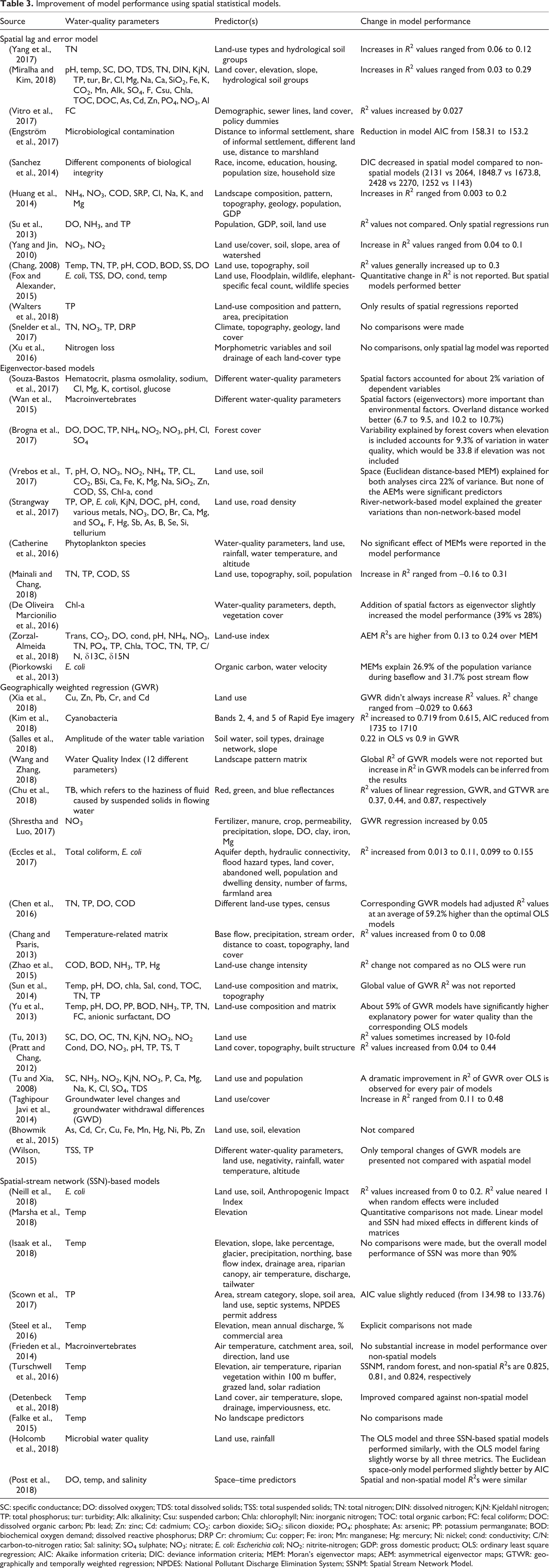
SC: specific conductance; DO: dissolved oxygen; TDS: total dissolved solids; TSS: total suspended solids; TN: total nitrogen; DIN: dissolved nitrogen; KjN: Kjeldahl nitrogen; TP: total phosphorus; tur: turbidity; Alk: alkalinity; Csu: suspended carbon; Chla: chlorophyll; Nin: inorganic nitrogen; TOC: total organic carbon; FC: fecal coliform; DOC: dissolved organic carbon; Pb: lead; Zn: zinc; Cd: cadmium; CO₂: carbon dioxide; SiO₂: silicon dioxide; PO₄: phosphate; As: arsenic; PP: potassium permanganate; BOD: biochemical oxygen demand; dissolved reactive phosphorus; DRP Cr: chromium; Cu: copper; Fe: iron; Mn: manganese; Hg: mercury; Ni: nickel; cond: conductivity; C/N: carbon-to-nitrogen ratio; Sal: salinity; SO₄ sulphate; NO₃: nitrate; E. coli: Escherichia coli; NO₂: nitrite-nitrogen; GDP: gross domestic product; OLS: ordinary least square regression; AIC: Akaike information criteria; DIC: deviance information criteria; MEM: Moran’s eigenvector maps; AEM: asymmetrical eigenvector maps; GTWR: geographically and temporally weighted regression; NPDES: National Pollutant Discharge Elimination System; SSNM: Spatial Stream Network Model.

V Conclusions

Spatial modeling of water quality is gaining increased attention, and researchers have been using novel and creative ways to incorporate spatial aspects into surface-water-quality modeling. Our review identifies a few aspects of these methods of modeling that stood out:

Research in this field is dominated by resource-rich countries like the US and China. This may be associated with the availability of data over a large geographical area.

There is still insufficient emphasis on spatial autocorrelation and RSAC, which deserve more attention as these techniques can help understand unidirectional, multidirectional, and river-network-based spatial attributes of the dependent variable and overall models of surface water quality. A suggestion based on this review would be to check for RSAC before performing spatial regression models if the researchers are concerned with the regression model not being able to account for the spatial autocorrelation.

Weights matrices have great potential in informing spatial autocorrelation of dependent variables at different scales, and in helping test several hypotheses of spatial eco-socio-hydrological processes in relation to surface water. Thus, testing the model’s sensitivity to different weights matrices needs further investigation. However, no study considered in our review has tested the sensitivity of a model against the changes in weight metrics.

Our reviews show that the modification of a weights matrix should be informed by spatial organization of water-quality data points, understanding of the source, mobilization, and delivery of a particular water-quality parameter, the hypothesis being tested, and the scale of analysis.

In most regression models except SSNs, predictor variables extracted from different scales are used differently to compare the model strength. A fusion of predictor variables extracted from different scales, such as in a multi-scale model, might be better suited to predict water quality, as different processes occur at several different scales simultaneously.

A thorough review of source, mobilization, delivery, and instream flow mechanism of the water-quality parameters under consideration might be necessary in order to include suitable predictor variables, multi-scale processes, and identify appropriate weights matrix in the model. This should be accompanied by proper variable reduction statistics, like brute-force reduction, in order to include manageable and meaningful predictors.

Although most of the spatial models recognize and incorporate the directional aspects of water flow, we did not find any papers using GWR. Researchers can attempt to modify GWR to incorporate directional process and river-network structures.

Researchers should also explore different spatial representations of the landscape matrix (e.g. composition, patterns, distance weighting, and hydrological weighting) in order to identify an appropriate approach to using them in the spatial modeling of water quality.

See Appendix 1 for a list of the software available for implementing the spatial statistical approaches reviewed in this paper.

Footnotes

Acknowledgements

We appreciate Dr. Anna Linton, who provided constructive comments on an earlier version of the manuscript. Barbara Brower and Alexander Ross at Portland State University helped improve the language of the manuscript. Views expressed are our own and do not necessarily reflect those of the sponsoring agency.

Declaration of conflicting interests

The author(s) declared no potential conflicts of interest with respect to the research, authorship and/or publication of this article.

Funding

The author(s) disclosed receipt of the following financial support for the research, authorship, and/or publication of this article: This material is based upon work supported by the US National Science Foundation NSF-GSS Grant #1560907.

ORCID iD

Heejun Chang

Appendix 1

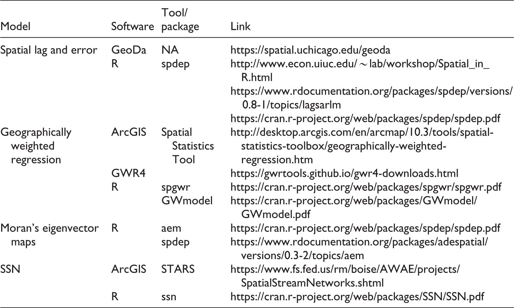
Model	Software	Tool/package	Link
Spatial lag and error	GeoDa	NA	https://spatial.uchicago.edu/geoda
Spatial lag and error	R	spdep	http://www.econ.uiuc.edu/∼lab/workshop/Spatial_in_R.html https://www.rdocumentation.org/packages/spdep/versions/0.8-1/topics/lagsarlm https://cran.r-project.org/web/packages/spdep/spdep.pdf
Geographically weighted regression	ArcGIS	Spatial Statistics Tool	http://desktop.arcgis.com/en/arcmap/10.3/tools/spatial-statistics-toolbox/geographically-weighted-regression.htm
	GWR4		https://gwrtools.github.io/gwr4-downloads.html
	R	spgwr	https://cran.r-project.org/web/packages/spgwr/spgwr.pdf
	R	GWmodel	https://cran.r-project.org/web/packages/GWmodel/GWmodel.pdf
Moran’s eigenvector maps	R	aem	https://cran.r-project.org/web/packages/spdep/spdep.pdf
Moran’s eigenvector maps	R	spdep	https://www.rdocumentation.org/packages/adespatial/versions/0.3-2/topics/aem
SSN	ArcGIS	STARS	https://www.fs.fed.us/rm/boise/AWAE/projects/SpatialStreamNetworks.shtml
SSN	R	ssn	https://cran.r-project.org/web/packages/SSN/SSN.pdf

References

Allan

(2004) Landscapes and riverscapes: The influence of land use on stream ecosystems. Annual Review of Ecology, Evolution, and Systematics 35(1): 257–284. DOI: 10.1146/annurev.ecolsys.35.120202.110122.

Anselin

(1988) Spatial Econometrics: Methods and Models. Kluwer Academic, Dordrecht.

Anselin

(1995) Local indicators of spatial association—LISA. Geographical analysis 27(2): 93–115.

Anselin

(2001) Spatial Econometrics. In: Baltagi

(ed.) A Companion to Theoretical Econometrics. New Jersey, USA: Blackwell Publishing Ltd., pp. 310–330.

Bhowmik

Alamdar

Katsoyiannis

, et al. (2015) Mapping human health risks from exposure to trace metal contamination of drinking water sources in Pakistan. Science of The Total Environment 538: 306–316. DOI: 10.1016/j.scitotenv.2015.08.069.

Bini

Diniz-Filho

JAF

Rangel

TFLVB

, et al. (2009) Coefficient shifts in geographical ecology: an empirical evaluation of spatial and non-spatial regression. Ecography 32(2): 193–204. DOI: 10.1111/j.1600-0587.2009.05717.x.

Blanchet

Legendre

Borcard

(2008) Modelling directional spatial processes in ecological data. Ecological Modelling 215(4): 325–336. DOI: 10.1016/j.ecolmodel.2008.04.001.

Borcard

Legendre

(2002) All-scale spatial analysis of ecological data by means of principal coordinates of neighbour matrices. Ecological Modelling 153(1): 51–68.

Brody

Highfield

Peck

(2005) Exploring the mosaic of perceptions for water quality across watersheds in San Antonio, Texas. Landscape and Urban Planning 73(2–3): 200–214. DOI: 10.1016/j.landurbplan.2004.11.010.

10.

Brogna

Michez

Jacobs

, et al. (2017) Linking forest cover to water quality: A multivariate analysis of large monitoring datasets. Water 9(3): 176. DOI: 10.3390/w9030176.

11.

Brunsdon

Fotheringham

Charlton

(1998) Geographically weighted regression. Journal of the Royal Statistical Society: Series D (The Statistician) 47(3): 431–443.

12.

Catherine

Selma

Mouillot

, et al. (2016) Patterns and multi-scale drivers of phytoplankton species richness in temperate peri-urban lakes. Science of The Total Environment 559: 74–83. DOI: 10.1016/j.scitotenv.2016.03.179.

13.

Chang

(2008) Spatial analysis of water quality trends in the Han River basin, South Korea. Water Research 42(13): 3285–3304. DOI: 10.1016/j.watres.2008.04.006.

14.

Chang

Psaris

(2013) Local landscape predictors of maximum stream temperature and thermal sensitivity in the Columbia River Basin, USA. Science of The Total Environment 461–462: 587–600. DOI: 10.1016/j.scitotenv.2013.05.033.

15.

Chen

Mei

Dahlgren

, et al. (2016) Impacts of land use and population density on seasonal surface water quality using a modified geographically weighted regression. Science of The Total Environment 572: 450–466. DOI: 10.1016/j.scitotenv.2016.08.052.

16.

Chu

H-J

Kong

S-J

Chang

C-H

(2018) Spatio-temporal water quality mapping from satellite images using geographically and temporally weighted regression. International Journal of Applied Earth Observation and Geoinformation 65: 1–11. DOI: 10.1016/j.jag.2017.10.001.

17.

Chun

(2014) Analyzing space–time crime incidents using eigenvector spatial filtering: an application to vehicle burglary. Geographical Analysis 46(2): 165–184. DOI: 10.1111/gean.12034.

18.

Cliff

Ord

(1972) Testing for spatial autocorrelation among regression residuals. Geographical analysis 4(3): 267–284.

19.

de Oliveira Marcionilio

SML

Machado

Carneiro

, et al. (2016) Environmental factors affecting chlorophyll-a concentration in tropical floodplain lakes, Central Brazil. Environmental Monitoring and Assessment 188(11): 611. DOI: 10.1007/s10661-016-5622-7.

20.

Detenbeck

Morrison

Abele

, et al. (2016) Spatial statistical network models for stream and river temperature in New England, USA. Water Resources Research 52(8): 6018–6040. DOI: 10.1002/2015WR018349.

21.

Eccles

Checkley

Sjogren

, et al. (2017) Lessons learned from the 2013 Calgary flood: Assessing risk of drinking water well contamination. Applied Geography 80: 78–85. DOI: 10.1016/j.apgeog.2017.02.005.

22.

Engström

Mörtberg

Karlström

, et al. (2017) Applying spatial regression to evaluate risk factors for microbiological contamination of urban groundwater sources in Juba, South Sudan. Hydrogeology Journal 25(4): 1077–1091. DOI: 10.1007/s10040-016-1504-x.

23.

Falke

Dunham

Hockman-Wert

, et al. (2016) A simple prioritization tool to diagnose impairment of stream temperature for coldwater fishes in the great basin. North American Journal of Fisheries Management 36(1): 147–160. DOI: 10.1080/02755947.2015.1115449.

24.

Fotheringham

Brunsdon

Charlton

(2002) Geographically Weighted Regression: The Analysis of Spatially Varying Relationships. Chichester, England; Hoboken, NJ, USA: Wiley.

25.

Fox

Alexander

(2015) Spatiotemporal variation and the role of wildlife in seasonal water quality declines in the chobe river, Botswana. PLOS ONE 10(10): e0139936. DOI: 10.1371/journal.pone.0139936.

26.

Frieden

Peterson

Angus Webb

, et al. (2014) Improving the predictive power of spatial statistical models of stream macroinvertebrates using weighted autocovariance functions. Environmental Modelling & Software 60: 320–330. DOI: 10.1016/j.envsoft.2014.06.019.

27.

Getis

Aldstadt

(2004) Constructing the spatial weights matrix using a local statistic. Geographical Analysis 36(2): 90–104. DOI: 10.1111/j.1538-4632.2004.tb01127.x.

28.

Getis

Griffith

(2002) Comparative Spatial Filtering in Regression Analysis. Geographical Analysis 34(2): 130–140. DOI: 10.1111/j.1538-4632.2002.tb01080.x.

29.

Getis

Ord

(1992) The analysis of spatial association by use of distance statistics. Geographical Analysis 24(3): 189–206. DOI: 10.1111/j.1538-4632.1992.tb00261.x.

30.

Giri

Qiu

(2016) Understanding the relationship of land uses and water quality in Twenty First Century: A review. Journal of Environmental Management 173: 41–48. DOI: 10.1016/j.jenvman.2016.02.029.

31.

Grabowski

Watson

Chang

(2016) Using spatially explicit indicators to investigate watershed characteristics and stream temperature relationships. Science of The Total Environment 551–552: 376–386. DOI: 10.1016/j.scitotenv.2016.02.042.

32.

Griffith

(2010) Spatial Filtering. In: Fischer

Getis

(eds) Handbook of Applied Spatial Analysis. Springer, Berlin, Heidelberg, pp. 301–318. DOI: 10.1007/978-3-642-03647-7_16.

33.

Griffith

Peres-Neto

(2006a) Spatial modeling in ecology: the flexibility of eigenfunction spatial analyses. Ecology 87(10): 2603–2613.

34.

Griffith

Peres-Neto

(2006b) Spatial modeling in ecology: the flexibility of eigenfunction spatial analyses. Ecology 87(10): 2603–2613.

35.

Guo

Lintern

Webb

, et al. (2019) Key factors affecting temporal variability in stream water quality. Water Resources Research 55(1): 112–129. DOI: 10.1029/2018WR023370.

36.

Holcomb

Messier

Serre

, et al. (2018) Geostatistical prediction of microbial water quality throughout a stream network using meteorology, land cover, and spatiotemporal autocorrelation. Environmental Science & Technology 52(14): 7775–7784. DOI: 10.1021/acs.est.8b01178.

37.

Huang

Zhang

(2014) Coupled effects of natural and anthropogenic controls on seasonal and spatial variations of river water quality during baseflow in a coastal watershed of southeast China. PLoS ONE 9(3): e91528. DOI: 10.1371/journal.pone.0091528.

38.

Huang

Han

Zeng

, et al. (2016) Effects of land use patterns on stream water quality: a case study of a small-scale watershed in the Three Gorges Reservoir Area, China. Environmental Science and Pollution Research 23(4): 3943–3955. DOI: 10.1007/s11356-015-5874-8.

39.

Isaak

Peterson

Ver Hoef

, et al. (2014) Applications of spatial statistical network models to stream data: Spatial statistical network models for stream data. Wiley Interdisciplinary Reviews: Water 1(3): 277–294. DOI: 10.1002/wat2.1023.

40.

Isaak

Ver Hoef

Peterson

, et al. (2017) Scalable population estimates using spatial-stream-network (SSN) models, fish density surveys, and national geospatial database frameworks for streams. Canadian Journal of Fisheries and Aquatic Sciences 74(2): 147–156. DOI: 10.1139/cjfas-2016-0247.

41.

Isaak

Wenger

Peterson

, et al. (2018) The norwest summer stream temperature model and scenarios for the western u.s.: a crowd-sourced database and new geospatial tools foster a user-community and predict broad climate warming of rivers and streams. Water Resources Research 53(11): 9181–9205. DOI: 10.1002/2017WR020969.

42.

Jackson

Malcolm

Hannah

(2015) A novel approach for designing large-scale river temperature monitoring networks. Hydrology Research 47(3): 569–590. DOI: 10.2166/nh.2015.106.

43.

Jacob

Muturi

Caamano

, et al. (2008) Hydrological modeling of geophysical parameters of arboviral and protozoan disease vectors in Internally Displaced People camps in Gulu, Uganda. International Journal of Health Geographics 7(1): 11. DOI: 10.1186/1476-072X-7-11.

44.

Kim

Shin

(2016) Spatial autocorrelation potentially indicates the degree of changes in the predictive power of environmental factors for plant diversity. Ecological Indicators 60: 1130–1141. DOI: 10.1016/j.ecolind.2015.09.021.

45.

Kim

Hirmas

McEwan

, et al. (2016) Predicting the Influence of Multi-Scale Spatial Autocorrelation on Soil–Landform Modeling. Soil Science Society of America Journal 80(2): 409. DOI: 10.2136/sssaj2015.10.0370.

46.

Kim

Seo

Baek

(2018) Modeling spatial variability of harmful algal bloom in regulated rivers using a depth-averaged 2D numerical model. Journal of Hydro-environment Research 20: 63–76. DOI: 10.1016/j.jher.2018.04.008.

47.

King

Baker

Whigham

, et al. (2005) Spatial considerations for linking watershed land cover to ecological indicators in streams. Ecological Applications 15(1): 137–153. DOI: 10.1890/04-0481.

48.

Legendre

(1993) Spatial autocorrelation: Trouble or new paradigm? Ecology 74(6): 1659–1673. DOI: 10.2307/1939924.

49.

Lintern

Webb

J a.

Ryu

, et al. (2018) Key factors influencing differences in stream water quality across space. Wiley Interdisciplinary Reviews: Water 5(1): e1260. DOI: 10.1002/wat2.1260.

50.

Liu

Zhang

Xia

, et al. (2016) Characterizing and explaining spatio-temporal variation of water quality in a highly disturbed river by multi-statistical techniques. SpringerPlus 5(1): 1171.

51.

Mainali

Chang

(2018) Landscape and anthropogenic factors affecting spatial patterns of water quality trends in a large river basin, South Korea. Journal of Hydrology 564: 26–40. DOI: 10.1016/j.jhydrol.2018.06.074.

52.

Marsha

Steel

Fullerton

, et al. (2018) Monitoring riverine thermal regimes on stream networks: Insights into spatial sampling designs from the Snoqualmie River, WA. Ecological Indicators 84: 11–26. DOI: 10.1016/j.ecolind.2017.08.028.

53.

McGuire

Torgersen

Likens

, et al. (2014) Network analysis reveals multiscale controls on streamwater chemistry. Proceedings of the National Academy of Sciences 111(19): 7030–7035. DOI: 10.1073/pnas.1404820111.

54.

McLean

Evers

Bowman

, et al. (2019) Statistical modelling of groundwater contamination monitoring data: A comparison of spatial and spatiotemporal methods. Science of The Total Environment 652: 1339–1346. DOI: 10.1016/j.scitotenv.2018.10.231.

55.

Miralha

Kim

(2018) Accounting for and predicting the influence of spatial autocorrelation in water quality modeling. ISPRS International Journal of Geo-Information 7(2): 64. DOI: 10.3390/ijgi7020064.

56.

Nature Statistics (2019) Statistical methods - Latest research and news | Nature. Available at: https://www.nature.com/subjects/statistical-methods (accessed 28 February 2019).

57.

Neill

Tetzlaff

Strachan

NJC

, et al. (2018) Using spatial-stream-network models and long-term data to understand and predict dynamics of faecal contamination in a mixed land-use catchment. Science of The Total Environment 612: 840–852. DOI: 10.1016/j.scitotenv.2017.08.151.

58.

Peterson

Sheldon

Darnell

, et al. (2011) A comparison of spatially explicit landscape representation methods and their relationship to stream condition. Freshwater Biology 56(3): 590–610. DOI: 10.1111/j.1365-2427.2010.02507.x.

59.

Peterson

Ver Hoef

Isaak

, et al. (2013) Modelling dendritic ecological networks in space: an integrated network perspective. Ecology Letters 16(5): 707–719. DOI: 10.1111/ele.12084.

60.

Piorkowski

Jamieson

Hansen

, et al. (2014) Characterizing spatial structure of sediment E. coli populations to inform sampling design. Environmental Monitoring and Assessment 186(1): 277–291. DOI: 10.1007/s10661-013-3373-2.

61.

Pond

Krock

KJG

Cruz

, et al. (2017) Effort-based predictors of headwater stream conditions: comparing the proximity of land use pressures and instream stressors on macroinvertebrate assemblages. Aquatic Sciences 79(3): 765–781. DOI: 10.1007/s00027-017-0534-3.

62.

Post

Cope

Gerard

, et al. (2018) Monitoring spatial and temporal variation of dissolved oxygen and water temperature in the Savannah River using a sensor network. Environmental Monitoring and Assessment 190(5). DOI: 10.1007/s10661-018-6646-y.

63.

Pratt

Chang

(2012) Effects of land cover, topography, and built structure on seasonal water quality at multiple spatial scales. Journal of Hazardous Materials 209–210: 48–58. DOI: 10.1016/j.jhazmat.2011.12.068.

64.

Salles

L de A

Lima

JEFW

Roig

, et al. (2018) Environmental factors and groundwater behavior in an agricultural experimental basin of the Brazilian central plateau. Applied Geography 94: 272–281. DOI: 10.1016/j.apgeog.2018.02.007.

65.

Sanchez

Nejadhashemi

Zhang

, et al. (2014) Development of a socio-ecological environmental justice model for watershed-based management. Journal of Hydrology 518: 162–177. DOI: 10.1016/j.jhydrol.2013.08.014.

66.

Schwarzenbach

Egli

Hofstetter

, et al. (2010) Global Water Pollution and Human Health. Annual Review of Environment and Resources 35(1): 109–136. DOI: 10.1146/annurev-environ-100809-125342.

67.

Scown

McManus

Carson

, et al. (2017) Improving predictive models of in-stream phosphorus concentration based on nationally-available spatial data coverages. JAWRA Journal of the American Water Resources Association 53(4): 944–960. DOI: 10.1111/1752-1688.12543.

68.

Shi

Zhang

, et al. (2017) Influence of land use and land cover patterns on seasonal water quality at multi-spatial scales. CATENA 151: 182–190. DOI: 10.1016/j.catena.2016.12.017.

69.

Shi

Xia

Zhang

(2016) Influences of anthropogenic activities and topography on water quality in the highly regulated Huai River basin, China. Environmental Science and Pollution Research 23(21): 21460–21474. DOI: 10.1007/s11356-016-7368-8.

70.

Shrestha

Luo

(2017) Analysis of groundwater nitrate contamination in the central valley: comparison of the geodetector method, principal component analysis and geographically weighted regression. ISPRS International Journal of Geo-Information 6(10): 297. DOI: 10.3390/ijgi6100297.

71.

Snelder

Larned

McDowell

(2018) Anthropogenic increases of catchment nitrogen and phosphorus loads in New Zealand. New Zealand Journal of Marine and Freshwater Research 52(3): 336–361. DOI: 10.1080/00288330.2017.1393758.

72.

Sokal

Oden

(1978) Spatial autocorrelation in biology: 1. Methodology. Biological journal of the Linnean Society 10(2): 199–228.

73.

Souza-Bastos

Bastos

Carneiro

PCF

, et al. (2017) Evaluation of the water quality of the upper reaches of the main Southern Brazil river (Iguaçu river) through in situ exposure of the native siluriform Rhamdia quelen in cages. Environmental Pollution 231: 1245–1255. DOI: 10.1016/j.envpol.2017.08.071.

74.

Steel

Sowder

Peterson

(2016) Spatial and temporal variation of water temperature regimes on the snoqualmie river network. JAWRA Journal of the American Water Resources Association 52(3): 769–787. DOI: 10.1111/1752-1688.12423.

75.

Strangway

Bowman

Kirkwood

(2017) Assessing landscape and contaminant point-sources as spatial determinants of water quality in the Vermilion River System, Ontario, Canada. Environmental Science and Pollution Research 24(28): 22587–22601. DOI: 10.1007/s11356-017-9933-1.

76.

Xiao

, et al. (2013) Multi-scale spatial determinants of dissolved oxygen and nutrients in Qiantang River, China. Regional Environmental Change 13(1): 77–89. DOI: 10.1007/s10113-012-0313-6.

77.

Sun

Guo

Liu

, et al. (2014) Scale effects on spatially varying relationships between urban landscape patterns and water quality. Environmental Management 54(2): 272–287. DOI: 10.1007/s00267-014-0287-x.

78.

Taghipour Javi

Malekmohammadi

Mokhtari

(2014) Application of geographically weighted regression model to analysis of spatiotemporal varying relationships between groundwater quantity and land use changes (case study: Khanmirza Plain, Iran). Environmental Monitoring and Assessment 186(5): 3123–3138. DOI: 10.1007/s10661-013-3605-5.

79.

Tobler

(1970) A computer movie simulating urban growth in the detroit region. Economic Geography 46: 234. DOI: 10.2307/143141.

80.

(2011) Spatially varying relationships between land use and water quality across an urbanization gradient explored by geographically weighted regression. Applied Geography 31(1): 376–392. DOI: 10.1016/j.apgeog.2010.08.001.

81.

(2013) Spatial variations in the relationships between land use and water quality across an urbanization gradient in the watersheds of northern georgia, USA. Environmental Management 51(1): 1–17. DOI: 10.1007/s00267-011-9738-9.

82.

Xia

(2008) Examining spatially varying relationships between land use and water quality using geographically weighted regression I: Model design and evaluation. Science of The Total Environment 407(1): 358–378. DOI: 10.1016/j.scitotenv.2008.09.031.

83.

Turschwell

Peterson

Balcombe

, et al. (2016) To aggregate or not? Capturing the spatio-temporal complexity of the thermal regime. Ecological Indicators 67: 39–48. DOI: 10.1016/j.ecolind.2016.02.014.

84.

Ullah

Jiang

Wang

(2018) Land use impacts on surface water quality by statistical approaches. Global Journal of Environment Science and Management 4(2): 231–250. DOI: 10.22034/gjesm.2018.04.02.010.

85.

Ver Hoef

Peterson

Clifford

, et al. (2014) SSN: An R package for spatial statistical modeling on stream networks. Journal of Statistical Software 56(3): 1–45.

86.

Ver Hoef

Peterson

(2010) A moving average approach for spatial statistical models of stream networks. Journal of the American Statistical Association 105(489): 6–18.

87.

Ver Hoef

Peterson

Theobald

(2006) Spatial statistical models that use flow and stream distance. Environmental and Ecological Statistics 13(4): 449–464. DOI: 10.1007/s10651-006-0022-8.

88.

Ver Hoef

Peterson

Hooten

, et al. (2018) Spatial autoregressive models for statistical inference from ecological data. Ecological Monographs 88(1): 36–59. DOI: 10.1002/ecm.1283.

89.

Vitro

BenDor

Jordanova

, et al. (2017) A geospatial analysis of land use and stormwater management on fecal coliform contamination in North Carolina streams. Science of The Total Environment 603–604: 709–727. DOI: 10.1016/j.scitotenv.2017.02.093.

90.

Vrebos

Beauchard

Meire

(2017) The impact of land use and spatial mediated processes on the water quality in a river system. Science of The Total Environment 601–602: 365–373. DOI: 10.1016/j.scitotenv.2017.05.217.

91.

Walters

Brody

Highfield

(2018) Examining the relationship between development patterns and total phosphorus in the Galveston Bay Estuary. Environmental Science & Policy 88: 10–16. DOI: 10.1016/j.envsci.2018.06.005.

92.

Wan

, et al. (2015) The role of environmental and spatial processes in structuring stream macroinvertebrates communities in a large river basin. CLEAN – Soil, Air, Water 43(12): 1633–1639. DOI: 10.1002/clen.201300861.

93.

Wang

Zhang

(2018) Multi-scale analysis of the relationship between landscape patterns and a water quality index (WQI) based on a stepwise linear regression (SLR) and geographically weighted regression (GWR) in the Ebinur Lake oasis. Environmental Science and Pollution Research 25(7): 7033–7048. DOI: 10.1007/s11356-017-1041-8.

94.

Wilson

(2015) Land use/land cover water quality nexus: quantifying anthropogenic influences on surface water quality. Environmental Monitoring and Assessment 187(7). DOI: 10.1007/s10661-015-4666-4.

95.

Xia

Wang

, et al. (2018) Distribution and source analysis of heavy metal pollutants in sediments of a rapid developing urban river system. Chemosphere 207: 218–228. DOI: 10.1016/j.chemosphere.2018.05.090.

96.

Yin

, et al. (2016) Spatiotemporal patterns of non-point source nitrogen loss in an agricultural catchment. Water Science and Engineering 9(2): 125–133. DOI: 10.1016/j.wse.2016.03.003.

97.

Yang

Jin

(2010) GIS-based spatial regression and prediction of water quality in river networks: A case study in Iowa. Journal of Environmental Management 91(10): 1943–1951. DOI: 10.1016/j.jenvman.2010.04.011.

98.

Yang

Liu

Luo

, et al. (2017) Spatial regression and prediction of water quality in a watershed with complex pollution sources. Scientific Reports 7(1). DOI: 10.1038/s41598-017-08254-w.

99.

, et al. (2016) Effect of land use types on stream water quality under seasonal variation and topographic characteristics in the Wei River basin, China. Ecological Indicators 60: 202–212. DOI: 10.1016/j.ecolind.2015.06.029.

100.

Zhao

Zhu

Sun

, et al. (2015) Water quality changes in response to urban expansion: spatially varying relations and determinants. Environmental Science and Pollution Research 22(21): 16997–17011. DOI: 10.1007/s11356-015-4795-x.

101.

Zhou

Peng

(2012) Assessing the effects of landscape pattern on river water quality at multiple scales: A case study of the Dongjiang River watershed, China. Ecological Indicators 23: 166–175. DOI: 10.1016/j.ecolind.2012.03.013.

102.

Zorzal-Almeida

Salim

Andrade

MRM

, et al. (2018) Effects of land use and spatial processes in water and surface sediment of tropical reservoirs at local and regional scales. Science of The Total Environment 644: 237–246. DOI: 10.1016/j.scitotenv.2018.06.361.