The development process of the Korean coastal mountain range: Examination from spatial distribution of knickzones

Abstract

Along the eastern margin of the Korean Peninsula, a coastal mountain range spanning over 800 km with summits above 1500 m faces the East Sea (or Sea of Japan), the back-arc sea behind the Japanese Islands. Two contrasting hypotheses exist regarding the tectonic history of this coastal mountain range: long-lasting and progressive uplifts from the Early Tertiary to the Late Quaternary, and a short and intensive uplift during the Early Miocene. However, to date, no consensus has been reached. Here, we studied the spatial distribution of knickzones to understand the formation period and development pattern of this coastal mountain range. We extracted the knickzones in a drainage basin from digital elevation models, and investigated whether or not they are transient knickzones induced by the development of the coastal mountain range. We found that all identified knickzones were stationary, which was verified by slope-area and chi-elevation analyses. This implies that sufficient time has passed for all transient knickzones relevant to the growth of the mountain range to migrate up to the catchment boundary and disappear. We then calculated the time spent for the migration of transient knickzones from the outlet to their stream heads to be at least 5.1 to 10.6 Myr. Therefore, our results suggest that the current form of the coastal mountain range had been built at least before 5.1 Myr ago and has reached a quasi-equilibrium state up to the present, thus invalidating the prevailing hypothesis of the long-lasting and progressive development until the Late Quaternary.

Keywords

Knickzone passive continental margin back-arc basin East Sea Taebaek Mountain Range coastal mountain range Korean Peninsula

I Introduction

The Korean Peninsula jutting out from the Eurasian continent is bordered in the east by the East Sea (or Sea of Japan), a back-arc sea behind the Japanese Island Arcs (Figure 1a). Along the eastern margin of the peninsula, there is a long coastal mountain range with steep escarpments facing the East Sea. The southern section of this range is called the Taebaek Mountain Range (TMR), while the northern section is named the Hamgyeong Mountain Range (HMR). The peaks on the coastal mountain range tend to increase in a northerly direction, the highest peak being 2500 m. The overall topography of the Korean Peninsula is closely related to this coastal mountain range. Therefore, understanding its orogenic process holds the key to explaining the development of the peninsula’s entire landscape.

Figure 1.

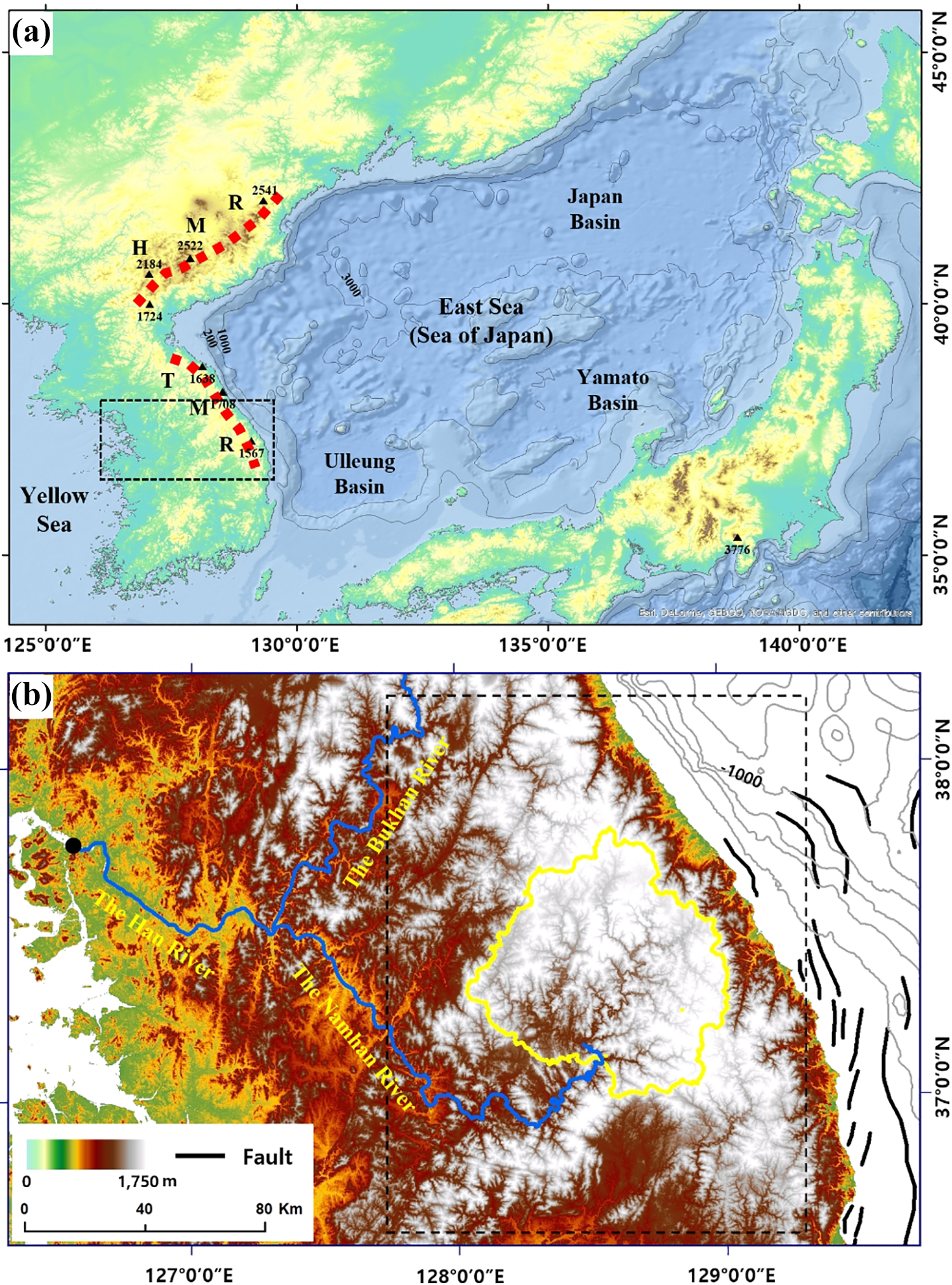
Coastal mountain range developed along the East Sea (1a) and DEM of the middle of the Korean Peninsula (1b). The inset boxes in Figures 1a and 1b indicate the extent of Figures 1b and 2, respectively. Note that inside the thick yellow line in Figure 1b is the study catchment. The Han River, a major river in South Korea, rises from the TMR, and flows westward across the middle of the peninsula, into which the studied rivers finally merge. The black dot (•) in Figure 1b is the outlet of the Han River. The East Sea, a back-arc sea consisting of abyssal basins, had opened through the following sequence (Hayashida et al., 1991; Jolivet and Tamaki, 1992; Jolivet et al., 1994; Kim et al., 2007; Lallemand and Jolivet, 1985; Otofuji, 1996; Otofuji et al., 1985; Tamaki et al., 1992; Yoon and Chough, 1995): crustal thinning and continental rifting in the current East Sea region since the Early Oligocene (23 to 32 Myr ago), active opening of the East Sea by back-arc basin extension (19 to 23 Myr ago), basin extension weakening (12 to 18 Myr ago), and closure of the East Sea since the late Middle Miocene (since 12 Myr ago). Although any Tertiary fault related to the formation of the TMR is not found in the peninsula (Kim, 1980), a series of faults relevant to the extension of the Ulleung Basin occur offshore nearly parallel to the coastline of the East Sea (Figure 1b, drawn based on Figure 7 in Yoon et al., 2014). If the coastal mountain range had formed intensively during the Early Miocene (Cho et al., 2018), they would be highly relevant to the building process of the coastal mountain range. For interpretation of the references to colours in this figure legend, refer to the online version of this article.

Two hypotheses exist regarding the timing of the mountain range formation. Early studies based on the depositional age of the Tertiary sedimentary rocks over the eastern margin of the peninsula and geomorphic features, such as erosional surfaces at different altitudes, suggested that the orogeny of the coastal mountain range had begun from the Early Tertiary, and persisted until the Late Quaternary; uplift had been continuous but four distinctive periods of higher uplift rates were present (Kim, 1961, 1973; Yoshikawa, 1947). This long-lasting and progressive formation hypothesis has prevailed (Kwon, 2000), presumably because several old publications have advocated this hypothesis. However, a recent study based on thermochronological data (i.e. apatite fission track and uranium-thorium/helium thermochronology) suggested that a short and intensive period of tectonic uplift during the Early Miocene near ca. 22 Myr ago is mainly responsible for the orogeny (Cho et al., 2018). The former hypothesis is based on the qualitative interpretation of topographic features but lacks quantitative evidence. In contrast, the latter hypothesis, based on thermochronological data, requires supporting geomorphic evidence. Thus, it remains an open question as to which hypothesis is closer to the truth.

Furthermore, the identification of the development period and pattern of the coastal mountain range is related to a question of what mechanisms lead to the growth of the orogenic belts in rifted passive margins. The orogenic timing proposed in the latter hypothesis matches the period when the East Sea had opened rapidly (23 to 19 Myr ago) (Kim et al., 2007; Yoon and Chough, 1995) (for the detailed history of the East Sea opening, refer to Figure 1 caption). This implies that, if the second hypothesis is to be accepted, the development of the coastal mountain range is mainly associated with the extension of the back-arc basin in the East Sea. On the other hand, if the first hypothesis is correct, the coastal mountain range would have formed progressively since the Early Oligocene even until the Late Quaternary, suggesting that the coastal mountain range had grown even until the closure period of the East Sea (12 Myr ago to the present). In that case, the long-lasting progressive development could be attributed to post-extension uplift mechanisms, such as isostatic rebounds due to mountain range denudation and consequent sedimentation in offshore regions (e.g. Gilchrist and Summerfield, 1990).

The purpose of this study is to better understand the development period of the coastal mountain range using new geomorphic evidence. Here, we investigated knickzones, which are substantially steeper channel reaches, within a catchment contained in the coastal mountain range. Knickzones can be classified as either stationary or transient (Wobus et al., 2006). Stationary knickzones often appear at static lithological boundaries between different rock types, while transient knickzones result from base-level lowering or sudden increase in uplift rate (Whipple and Tucker, 1999). We investigated the present distribution of transient knickzones, as this could lead to understanding the formation period of the coastal mountain range.

Within a homogeneous catchment, where physical variables determine the rate of headwater knickzone propagation, transient knickzones located on individual tributaries but originating from a common tectonic event tend to be at a similar altitude at any time during their upstream propagation (Niemann et al., 2001). Thus, the presence and location of transient knickzones within a catchment reflect tectonic uplift history. We adopted this notion and investigated the distribution and characteristics of knickzones within a catchment bounded by the TMR to understand the development period and pattern of the coastal mountain range.

The rest of this paper is organized as follows: a study catchment selected for this study is introduced in Section 2, various methods utilized in this study are reviewed and described in Section 3, and analysis results and discussions are given in Sections 4 and 5, respectively. Finally, summary and conclusions are presented in Section 6.

II Study area

The Korean Peninsula resides on the Amurian Plate in northeast Asia, which was once considered a part of the Eurasian Plate and is bounded to the east by the Okhotsk Plate beneath which the Pacific Plate is subducting and to the southeast by the Philippine Sea Plate. The peninsula is surrounded by the East Sea and the Yellow Sea. The coastal mountain range, the backbone mountain range of the peninsula, extends from the Asia continent toward the south along the peninsula’s eastern margin. It thus separates the peninsula into a narrow, steep eastern side that forms long escarpments facing the East Sea and a broad, gentler slope on the western side.

Regarding the orogenic process of the NNW-SSE trending TMR, up-warping was first suggested because any surface deformation relevant to the TMR formation, that is, Tertiary faults, was not observed over the peninsula (Kim, 1980) (Figure 1b). Recently, syn-rift flank uplift associated with back-arc basin rifting was proposed based on the thermochronological data from the TMR, in which an intense exhumation period corresponds to the opening of the East Sea (Cho et al., 2018). These assertions, however, do not explain clearly what mechanism caused the orogenic process.

To obtain a clear spatial distribution of knickzones, we chose a catchment located on the western side of the TMR, namely the upper Namhan River basin, as the study catchment with an area of 4769 km² (Figure 2). A large catchment with many tributaries is preferred because such a region is expected to be characterized by a large number of knickzones. Compared with the eastern side of the coastal mountain range, the western side exhibits a gentler slope, leading to the formation of bigger catchments with more and longer tributaries.

Some caution may be needed when interpreting tectonic uplift based on transient knickzone data. All tectonic episodes that the transient knickzones in the study area have recorded could not result directly from the TMR orogeny. Erosion and sediment loading even during the orogenic process could induce a surface deformation; for example, differential uplift due to block tilting in an extensional normal fault system (Pechlivanidou et al., 2019).

In the case of the Korean Peninsula, however, any deformation related to flexural response has not been reported yet. In addition, the west coast of the peninsula, where the rivers in the study area flow toward (Figure 1b) and thus transient knickzones due to the TRM orogeny would form and begin to progress, shows coastal terraces aligned to the level of those in the east coast, implying that the western margin of the peninsula has been uplifted as well (Choi and Lee, 2007). Furthermore, a recent study based on the cosmogenic nuclides dating method suggested that the west coastline has been tectonically stable since the last interglacial stage (Choi et al., 2012). These prove that surface deformation like tilting across the peninsula has been limited. Accordingly, the transient knickzones identified in the study area are reliable evidence for understanding the TMR orogeny.

Among many catchments on the western side of the coastal mountain range, the study catchment is most advantageous from the perspective of knickzone analysis because catchments adjacent to the TMR (located in South Korea) have more detailed geological information; moreover, high-resolution satellite images of the area are available to assess the causes of knickzone formation and classify knickzones, in comparison with those along the HMR (located in North Korea). On the other hand, many catchments adjacent to the TMR are heavily developed, and several streams are blocked by large dams that limit the recognition of its upstream knickzones. However, our study catchment is a rare area in that only a few small dams exist. For these reasons, our study catchment had also been chosen in previous studies pertaining to the orogeny of the coastal mountain range (Kim, 1961, 1973; Song, 1998).

The study catchment shows a high relief, with an elevation ranging between 175 and 1540 m a.s.l. (Figure 2). The elevation tends to be higher in the east, where high-altitude plateaus and high summits are present. Notably, the granite areas (Figure 2, inset), where deeply weathered saprolites dominate, show low-relief hilly landscapes compared to the high-relief areas underlain by sedimentary and metamorphic rocks.

Figure 2.

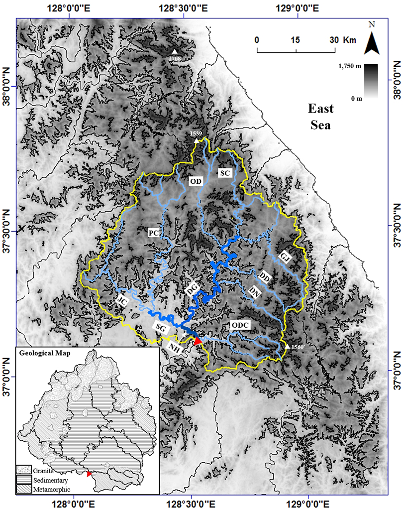
Study catchment of the upper Namhan River (inside the thick yellow line). Stream branches examined for knickzones are of bluish lines, and the red triangle is the outlet of the study catchment. Initials of major stream branches are given as follows: the Namhan River (NH) of the thickest deep blue line, and the Dong (DG), Seo (SG) Rivers of thick blue lines, and the Golji (GJ), Dongdae (DD), Dongnam (DN), Ocdong (ODC), Song (SC), Odae (OD), Pyeongchang (PC), and Ju (JC) Rivers of thin sky-blue lines. For the color image, refer to the online version of this article.

III Methods

To address the purpose of this study, we investigated the distribution of transient knickzones in the study catchment. If the coastal mountain range was formed by a sustained uplift scenario with multiple periods of accelerated uplift until the Late Quaternary (Figure 3a), a series of multiple transient knickzones would have formed at different altitudes along each tributary in the study catchment (Figure 3c). In contrast, if an intensive tectonic uplift, concentrated over a relatively short period of time, had resulted in the formation of the mountain range (Figure 3b), most transient knickzones should be found at approximately the same altitude from the datum (Figure 3d). Alternatively, transient knickzones would have arrived at stream heads and disappeared if sufficient time had passed since the last intensive uplift. Thus, the identification of transient knickzones and their accurate locations in the study catchment is primarily required. The calculation of the period for any transient knickzone’s migration to its present position is also needed because it allows us to estimate the minimum age of the last enhanced tectonic activity.

Figure 3.

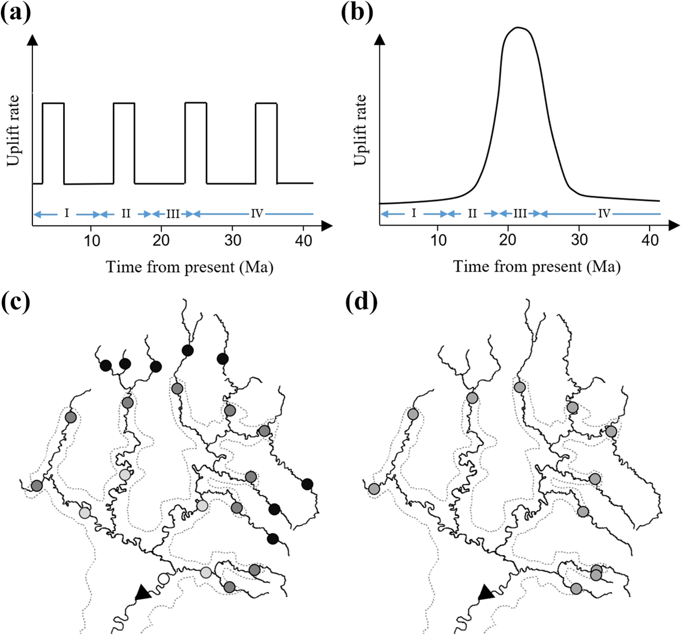
Schematics for the assertions on the uplift history of the coastal mountain range (Figure 3a, a long-lasting development with multiple periods of accelerated uplift, and Figure 3b, a short and intensive period of uplift), and their plausible resultant patterns for transient knickzones in the study catchment (circles in Figures 3c and 3d). I, II, III, and IV in Figures 3a and 3b correspond to four periods of the East Sea opening, i.e., the closure of the East Sea, back-arc basin extension weakening, rapid opening of the East Sea, and continental rifting, respectively (for detail, refer to the caption of Figure 1). Note that a circle can have more than one knickzone, and that the transient knickzones of the same color indicate that the same tectonic event induced them. The triangle and the dotted grey line in Figures 3c and 3d indicate the catchment outlet and a contour line of about 550 m, respectively.

For the identification of knickzones and their accurate locations, we used the relative steepness index, proposed by Hayakawa and Oguchi (2006) (see Section 3.1). The power-law relationship between slope and drainage area is often used to identify knickzones (Wobus et al., 2006). However, locating knickzones precisely based on the slope-area relation is challenging because the identified location tends to vary with the chosen channel concavity index value (Kirby and Whipple, 2012). The method of Hayakawa and Oguchi (2006) is expected to exhibit less variability as it relies only on channel slope data for locating knickzones. At the scale of an entire drainage basin, however, the slope-area analysis has been widely used to assess landscape transience or equilibrium (Kirby and Whipple, 2012). To assess the landscape transience of the study catchment, we applied the slope-area analysis as well as chi-elevation analysis designed to resolve the uncertainty due to noisy channel slope data (Perron and Royden, 2013) (see Section 3.2). Lastly, the method to estimate the propagation period of transient knickzone is given in Section 3.3.

3.1 Identification of transient knickzone

Transient knickzones were identified in four steps: extraction of longitudinal channel profiles, identification of knickzone candidates based on stream gradient variation, selection of true knickzones among the candidates, and classification of transient knickzones among those selected. Below, each of these steps is described in detail.

Step 1: Extraction of longitudinal profile

Terrain analysis using a digital elevation model (DEM) was utilized to extract longitudinal profiles of all major stream branches (e.g. Figure 4a). The shuttle radar topographic mission (SRTM) 1 arc-second (approximately 30 m horizontal resolution and 1 m vertical resolution) DEM was used. We used the algorithm of Byun and Seong (2015), which utilizes the raw sink-unfilled DEM, and is known to provide longitudinal profiles closer to those obtained via manual extraction. Along each profile, a channel head is determined as a point where initiation of concavity (or convergence in plan-form) is found in 1:25000 topographic contour map published by the National Geographic Information Institute of Korea. Such initiation occurs at the upslope area corresponding to two or three DEM cells (about 1800 and 2700 m²) for all branches we investigated.

Figure 4.

Demonstration for defining knickzone candidates based on R_d . Figure 4a shows the entire longitudinal profile of the branch DD, which begins from the channel head of the DD, and ends at the outlet of the study catchment (for the DD location, see Figure 2). Figures b–d show the longitudinal profile, stream gradient values calculated with varying distance D, and the degree of change in a series of stream gradient values at every cell, R_d , respectively, for a short segment of the entire river profile (inside the rectangular box in Figure 4a). Note that the channel reaches marked with thick line in Figure 4b are knickzone candidates above 1.5 R_d Z-score, the grey dotted line in Figure 4d. The R_d value at the black dot on the horizontal axis in Figure 4c, 4.7x10^-6, is the absolute slope value of the regressed line in the inset box in Figure 4c. For interpretation of the references to colours in this figure legend, refer to the online version of this article.

Like any DEM, 1 arc-second SRTM DEM has a limited resolution, although this has a far greater resolution than its predecessor of 3 arc-second. There is a concern that such a limitation could influence analysis results. For the scope of this study, the risk associated with using a poor resolution DEM is that some knickzone candidates may be neglected. We acknowledge this risk and have kept this in consideration while implementing the rest of the analysis. Nevertheless, we advocate the use of 1 arc-second SRTM DEM because we aimed to detect knickzones, rather than knickpoints that are discrete features often with a horizontal length of less than 30 m. A knickzone can reach up to several hundred meters in length (Hayakawa and Oguchi, 2006, 2009) and consists of high gradient cascade reach, commonly including a series of knickpoints (Ortega et al., 2013; Phillips et al., 2010). In fact, 1 or 3 arc-second SRTM DEMs have been actively used for the analysis of transient knickzones despite the concerns described previously (e.g. Kirby and Whipple, 2012; Wang et al., 2017).

Step 2: Identification of knickzone candidates

We detected virtually all knickzone candidates along all major tributaries within the study catchment using the relative steepness index, following the procedure below (for illustration, see Figure 4). First, a series of stream gradient values, G(x, D), for varying base distance D, are calculated at every cell (or node) along each branch as

G (x, D) = \frac{z (x - D / 2) - z (x + D / 2)}{D} (x_{c} \leq x \leq L),

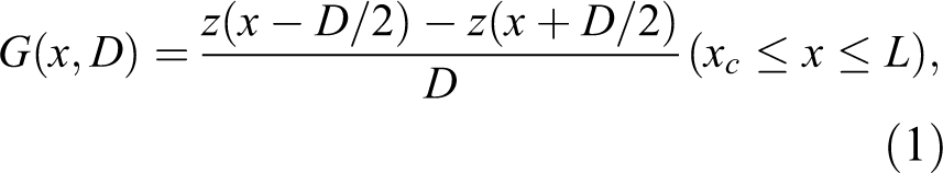
where z(x) = the elevation of a cell that is at x distance from a channel head; D = the arbitrary horizontal displacement; x_c = the distance from the drainage divide to the channel head; and L = the entire stream length of a chosen river from a channel head to a given outlet.

The relation between G and D at a cell represents any systematic tendency between local slope based on a short D and general slope over a longer D. For the special case of a linear longitudinal profile, G shows no variation with D. Other than that, G increases or decreases with D. For the case of a knickzone, a substantial decrease of G with D is expected. Here, we used a set of values of 1.1, 1.4, 1.7, 2.0, 2.3, 2.6, and 2.9 km as D. The minimum D value for a local slope was set as 1.1 km because D below 1.1 km yields negative G(x, D) in cases (often due to a sink in DEM), which is unrealistic. For the maximum D value for a general slope, 2.9 km was chosen where the standard deviation for all G values along each profile begins to rise with increasing D. Hence, G based on the maximum D could represent a general slope, but not reflect the channel concavity.

At every cell, along the distance x of each branch, we calculated the variation of G(x, D) with D (Figure 4c). Claiming a linear fitness between G and D, we expect G∝-R_dD (Figure 4c, inset) where the slope R_d is called the relative steepness index. Cells with high R_d values are potential knickzone candidates (Figure 4d). In the beginning, we assumed a 1.5 R_d Z-score (equivalent to a R_d value = mean R_d + 1.5 times of the standard deviation of R_d ), as the threshold value for distinguishing a knickzone candidate. In particular, to obtain practical statistics of R_d for the chosen rivers, we excluded the cells with exceptionally high R_d values owing to man-made structures, such as dams, before calculating the mean R_d .

Step 3: Selection of true knickzone

The candidates obtained via Step 2 are solely based on DEM analysis and could be erroneously selected due to various reasons such as the inherent errors in the DEM and the uncertainty in the threshold R_d value. The candidates can also be other features with sudden local geomorphic variation similar to knickzones, such as artificial structures, bars (point, alternate, mid-channel), and bedrock islands. Accordingly, we carefully investigated every knickzone candidate and removed the erroneously detected ones. It was possible to check many of these through analysis of high-quality aerial images, provided by Google Earth and Daum Map (http://map.daum.net), and ground truth field surveys. This resulted in the elimination of many knickzone candidates that were, in reality, channel bars.

Step 4: Classification of transient knickzones

Each identified knickzone was classified as either stationary or transient. We thoroughly checked whether the identified knickzones are stationary following three criteria: geologic boundary, local erodibility difference, and coarse sediment supply from a tributary. The remaining knickzones, unfiltered by the above criteria, were to be classified as transient. The criteria to classify stationary knickzones were compiled from existing literature (Hanks and Webb, 2006; Wobus et al., 2006).

Stationary knickzones appear where bedrock erodibility shows sharp contrast. Such contrasts are often found at the boundary between different rock types (Wobus et al., 2006). They can also be found at rock bodies, which exhibit a difference in erodibility but are not distinguished in the geological map (i.e. marked as the same rock type with surrounding terrain). Stationary knickzones can also form over a channel junction where a tributary supplies coarser sediment, and hence impedes sediment transport (Hanks and Webb, 2006). Active faults can also make and maintain stationary knickzones (Wobus et al., 2006). These cases are eliminated here because no active fault has been reported across the study catchment, compared with the southeastern margin of the peninsula (Kim et al., 2011; National Emergency Management Agency, 2011; Park et al., 2006).

We used the 1:50000 geological map provided by the Korea Institute of Geoscience and Mineral Resources (https://mgeo.kigam.re.kr) to assess whether each identified knickzone is adjacent to a geologic boundary between different rock types. Checking stationary knickzones due to local erodibility difference requires additional work. If an identified knickzone is indeed transient, other transient knickzones formed by the same tectonic event should exist at a similar altitude in adjacent tributaries (Niemann et al., 2001). Hence, for every knickzone unfiltered by two criteria of geologic boundary and channel junction, we determined whether it is transient by searching other knickzones in adjacent branches at a similar altitude. In the absence of any other knickzone at a similar altitude, the identified knickzone was considered to be formed as a result of locally different erodibility. Stationary knickzones relevant to channel junctions were checked using the flow paths obtained from DEM or satellite images.

3.2 Assessment of landscape transience: slope-area and chi-elevation analyses

The power-law relationship of slope and drainage area has been used to identify transient knickzones that are a signal of landscape transience (Kirby and Whipple, 2012). It was induced from a clear geometric relationship between the local slope S and drainage area A along a river (Flint, 1974) as

S = k_{s} A^{- θ},

where k_s = the channel steepness index describing the overall gradient of a river profile; and θ = the channel concavity index indicating how concave a river profile is. Note that S corresponds to a limit value of G in equation (1) as D approaches 0 but practically is approximated by G value based on the minimum D in this study.

Equation (2) can be analytically obtained for a detachment-limited stream in steady-state, using the stream power incision model (Whipple and Tucker, 1999)

\frac{d z}{d t} = U - k A^{m} S^{n},

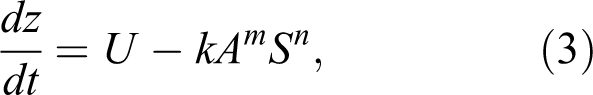
where t = the time; and U = the uplift rate. Here, k = the erodibility coefficient that depends on lithology, climate, and sediment load; and m and n = exponents that are dependent on bedrock channel erosion processes (Whipple et al., 2000). Under a circumstance where U and k are uniform throughout a channel reach, and erosion on a channel bed is in equilibrium with uplift (dz/dt = 0), a power-law relation of slope and drainage area, similar to equation (2), is identified as

S = (\frac{U}{k})^{1/n} A^{- m / n}

where, comparing equations (2) and (4), (U/k)^1/n = the channel steepness index k_s ; and m/n = the channel concavity index θ.

Accordingly, a well-defined inverse power-law relationship could emerge from steady-state topography region balancing uplift rate with erosion rate (e.g. Snyder et al., 2000). Conversely, a poor relationship was demonstrated under the catchment with no uplift case, although it resulted from the transport-limited condition (Willgoose, 1994). Indeed, the slope-area analysis has been widely applied to validate equilibrium landscapes or identify tectonic landscape transience (e.g. Kirby and Whipple, 2012; Montgomery, 2001).

To address the well-known uncertainty of channel slope data, mainly resulting from DEM errors (Wobus et al., 2006), Perron and Royden (2013) introduced a transformed river profile by replacing noisy slope data with elevation via integrating both sides of equation (2), which can be shown as

z = z_{o} + (\frac{k_{s}}{A_{0}^{θ}}) χ,

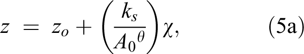
where z_o = the catchment outlet elevation, and

χ = \int_{0}^{x} {(\frac{A_{0}}{A (x)})}^{θ} d x,

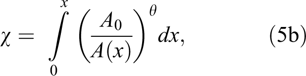
where A₀ = the reference upstream area used to non-dimensionalize the area term, which is usually set to unity (i.e. 1 km²).

Note that equation (5a) shows a linear relation of elevation with χ, similar to the linear relationship between slope and drainage area in the log–log scale. Thus, abrupt transition in the slope of the χ-transformed river profile in equation (5a) has also been used as a landscape transience signal (Beeson et al., 2017; Perron and Royden, 2013; Whipple et al., 2017). For the assessment of landscape transience, we drew chi-elevation plots as well as a slope-area relation curve for the studied rivers.

3.3 Estimation of the migration period of transient knickzone

Tectonic forcing leads to the formation of transient knickzones that migrate upstream over time (e.g. Berlin and Anderson, 2007; Crosby and Whipple, 2006). When a bedrock channel in steady-state is perturbed by a sudden increase in tectonic uplift rate, the channel adjusts to the enhanced uplift rate by increasing the channel slope, and then forms a steep transient knickzone separating the adjusted downstream reaches from upstream reaches that have not yet responded to the accelerated tectonic forcing (Whipple and Tucker, 1999). Thus, as transient knickzones migrate headward, a wave of incision also propagates through the upper rest of the catchment.

Theoretical and field-based studies have demonstrated that headward knickzone propagation is governed by the stream power erosion law and thus the knickzone retreat rate can be approximated by (Whittaker and Boulton, 2012; Whipple and Tucker, 1999)

\frac{d x}{d t} = - k A^{m} S^{n - 1} .

Rearranging the terms in equation (6) and integrating both sides provides an estimation of a period for knickzone migration from the datum as

T_{d} = | - \int_{0}^{L - x_{k}} \frac{1}{k A^{m} S^{n - 1}} d x |,

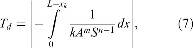
where x_k = the distance of an identified knickzone from the channel head; and T_d = the duration of a migrating knickzone from the outlet to a modern knickzone location.

The unknown parameter k in equation (7), which is the same as the coefficient k in equation (3), represents the channel bed erodibility. Here, if we assume that the path along which a transient knickzone migrates is in steady-state (dz/dt=U), we could yield k value at each node along the knickzone migration path using equation (3), which can be shown as

k = \frac{U}{A^{m} S^{n}}

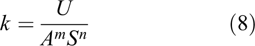
Lastly, substituting k in equation (7) with equation (8) leads to equation (9) for estimating knickzone migration period, which is determined by the uplift rate of the study area and local channel slope, regardless of the exponent m and n in the stream power incision model, and can be shown as

T_{d} = | - \int_{0}^{L - x_{k}} \frac{S}{U} d x |

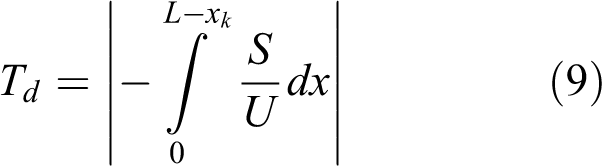
where U can be approximated by erosion rate where the landscape is in steady-state; and the S value at every node is acquired from the DEM along the chosen river.

IV Results

4.1 Knickzone distribution and classification

Through the calculation of the relative steepness index R_d , we found 62 knickzone candidates whose R_d Z-scores exceed the threshold value of 1.5. Detailed screening filtered out many of these, and 18 true knickzones were verified (Table 1, Figure 5). The length of a knickzone was approximated by summing the distance of each cell of the knickzone. The mean gradient was obtained by dividing the elevation gap of the knickzone with its length. The average length and gradient of the 18 true knickzones were 689 m and 0.04, respectively (Table 2). Their mean R_d Z-score was 2.51 (corresponding to the R_d value of 4.4×10^-6). This mean R_d value is nearly one-tenth of that of the Japanese mountainous catchments analyzed by Hayakawa and Oguchi (2009), implying that clear knickzones like those found in the Japanese sites rarely exist in our study catchment.

Figure 5.

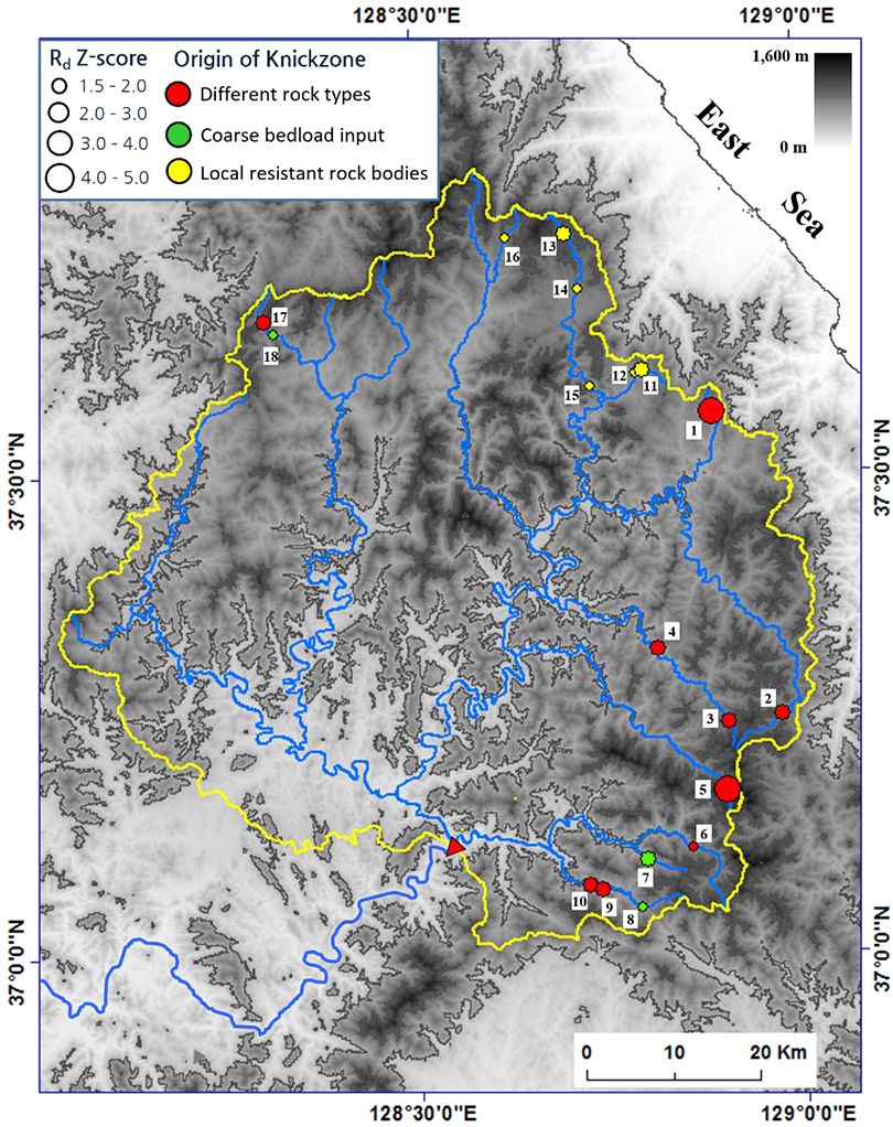
Spatial distribution of the verified knickzones with different origins and varying R_d Z-score (for detailed information of each knickzone, refer to Table 1). For interpretation of the references to colours in this figure legend, refer to the online version of this article.

Table 1.

Verified true knickzones in the study catchment (for the location of each knickzone, refer to Figure 5).

No.	Coordinates^a (WGS84)		R_d ^b	R_d Z-score^b	Elevations of upper and lower bounds (m)	ElevationDrop (m)	Length(m)	Mean knickzone gradient	Channel bed morphology	Cause of knickzone formation^c
1	37.564861°	128.888738°	8.33 x10^-6	4.69	705 / 617	88	1,082	0.081	step-pool & cascade	DRT
2	37.249306°	128.972072°	4.19 x10^-6	2.40	804 / 790	14	711	0.020	cascade & bedrock dominated	DRT
3	37.242634°	128.902190°	4.77 x10^-6	2.72	819 / 735	84	804	0.104	cascade & bedrock dominated	DRT
4	37.319055°	128.811314°	4.40 x10^-6	2.51	525 / 512	13	649	0.020	bedrock dominated	DRT & ancient fault line
5	37.170695°	128.899874°	8.62 x10^-6	4.85	1,022 / 919	103	989	0.104	cascade	DRT
6	37.112756°	128.852626°	3.36 x10^-6	1.94	624 / 604	20	866	0.023	cascade & bedrock dominated	DRT
7	37.100589°	128.794359°	4.76 x10^-6	2.71	524 / 488	36	680	0.053	cascade	CBLI
8	37.050278°	128.786794°	3.22 x10^-6	1.86	609 / 603	6	340	0.018	cascade	CBLI
9	37.069298°	128.735277°	4.80 x10^-6	2.74	484 / 454	30	1,020	0.029	step-pool & cascade	DRT
10	37.073988°	128.719732°	4.10 x10^-6	2.35	435 / 418	17	618	0.028	step-pool & cascade	DRT
11	37.609305°	128.797072°	3.73 x10^-6	2.15	724 / 712	12	495	0.024	cascade & bedrock dominated	LRRB
12	37.606250°	128.789016°	3.28 x10^-6	1.89	687 / 681	6	433	0.014	cascade & bedrock dominated	LRRB
13	37.751250°	128.699433°	3.91 x10^-6	2.24	975 / 943	32	897	0.036	cascade & bedrock dominated	LRRB
14	37.694583°	128.715544°	3.30 x10^-6	1.91	768 / 759	9	587	0.015	cascade & bedrock dominated	LRRB
15	37.592083°	128.730127°	3.28 x10^-6	1.90	636 / 625	11	402	0.027	bedrock dominated	LRRB
16	37.747361°	128.622072°	3.09 x10^-6	1.79	776 / 752	24	587	0.041	cascade & bedrock dominated	LRRB
17	37.664305°	128.304572°	4.56 x10^-6	2.60	714 / 690	24	835	0.029	step-pool & bedrock-dominated	DRT
18	37.650694°	128.316238°	3.35 x10^-6	1.94	651 / 638	13	402	0.032	riffle-pool	CBLI

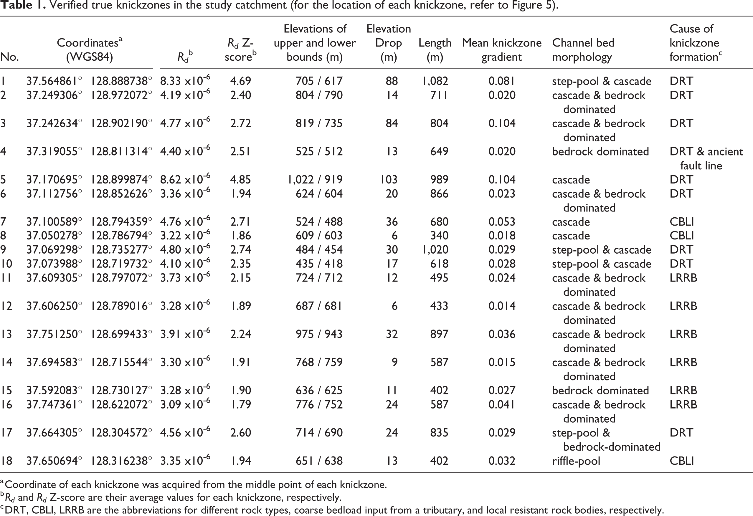
^a Coordinate of each knickzone was acquired from the middle point of each knickzone.

^b R_d and R_d Z-score are their average values for each knickzone, respectively.

^c DRT, CBLI, LRRB are the abbreviations for different rock types, coarse bedload input from a tributary, and local resistant rock bodies, respectively.

Table 2.

Statistics of the knickzones in the study catchment.

	All knickzones	Causes of knickzone formation
	All knickzones	Different rock types	Input of coarse bed materials from a tributary	Local resistant rock bodies
Number	18	9	3	6
Mean Rd	(4.4±1.6) x 10^-6	(5.2±1.8) x 10^-6	(3.8±0.7) x 10^-6	(3.4±0.3) x 10^-6
Mean Rd Z-score	2.51±0.86	2.98±0.99	2.17±0.39	1.98±0.16
Mean length (m)	689±221	842±155	474±148	567±163
Mean gradient	0.039±0.028	0.049±0.035	0.034±0.014	0.026±0.010

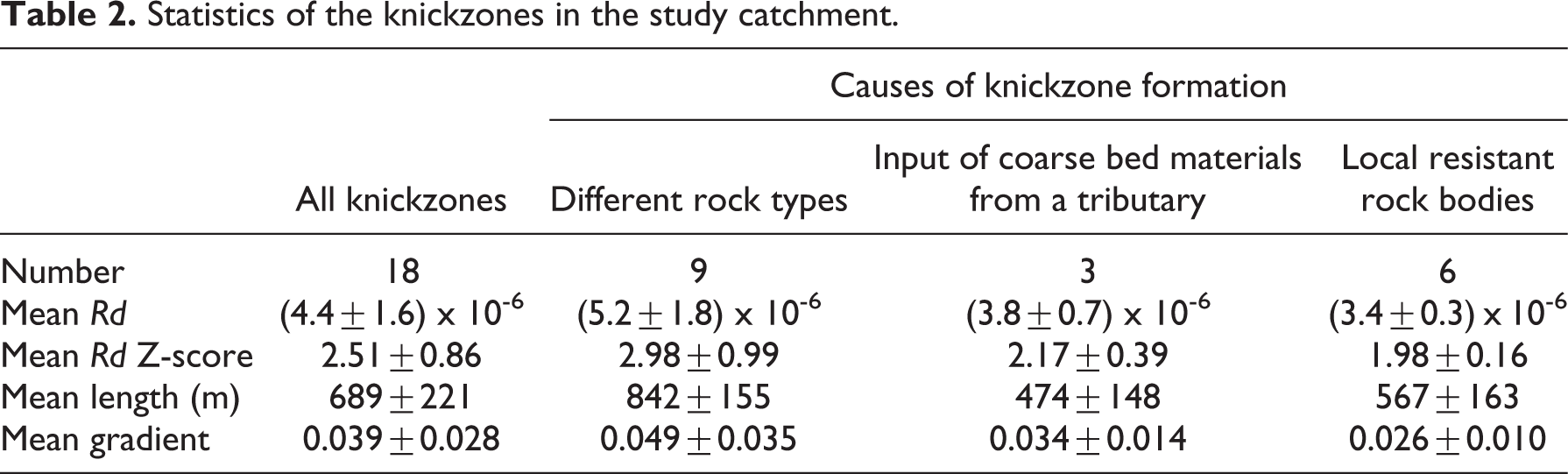
Most knickzones were within the elevation range between 600 and 800 m (Figure 6). This raises a suspicion that those are transient knickzones that originated from a common tectonic forcing, or tectonic events that occurred for a short period of time. However, we found that all identified knickzones were stationary knickzones not relevant to the growth of the coastal mountain range. Half of them (i.e. 9) were associated with the geological boundary between different rock types, and showed greater mean length and R_d value than others (Figure 7 and Table 2). The remaining knickzones were associated with either coarse bedload inputs from a tributary (3 knickzones) or locally resistant rock bodies (6 knickzones) (Table 2).

Figure 6.

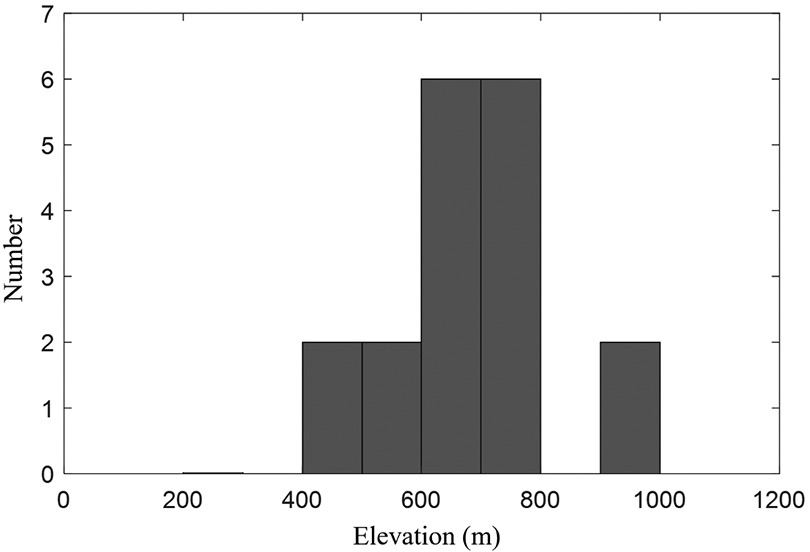
Altitudinal distribution of all identified knickzones.

Figure 7.

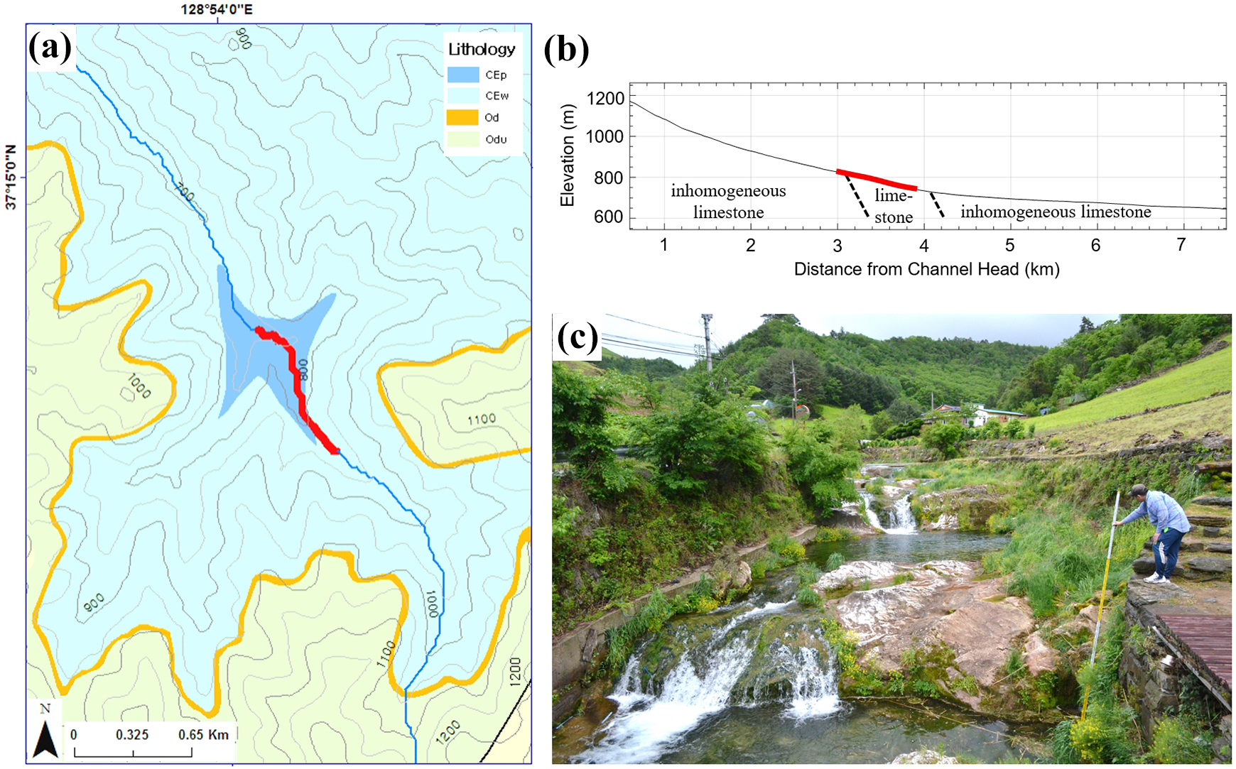
A knickzone over a boundary between different rock types, thick red line in Figures 7a and 7b (no. 3 knickzone in Table 1 and Figure 5), is of bedrock cascade beds (Figure 7c). CEp in Figure 7a is pure limestone, CEw and Odu are inhomogeneous limestones including shale and slate, and Od is quartzite. For interpretation of the references to colours in this figure legend, refer to the online version of this article.

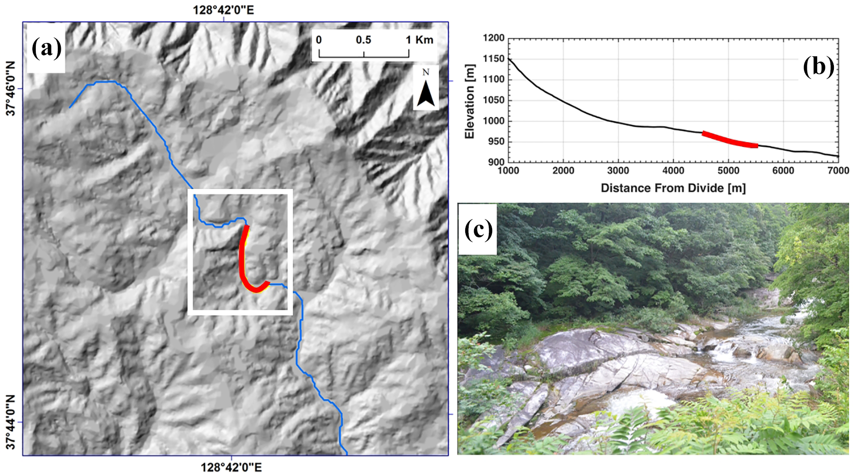
The knickzones occurring at channel junctions are mostly composed of coarse materials like cobble and boulder-sized clasts. A knickzone formed by the accumulation of such coarse bed materials transferred from a tributary is usually due to a lithological difference between the drainage basins of the main trunk and a tributary (Hanks and Webb, 2006). However, the geological map we used did not show such lithological difference for our three knickzones found at channel junctions. Instead, they were found where steep and low-order tributaries meet wider channels and their bed materials were similar in size to those consisting of the knickzone (Figure 8). Thus, we postulate other reasons behind the size difference in bed materials such as landslides from steep and low-order channels. For example, during the summer monsoon season in Korea, coarse bed materials in the steep and low-order channels, mostly composed of colluvial and step-pool channel reaches, are transferred rapidly by debris flows to the junctions with gentle and high-order channels and then inhibit fluvial transportation of the high-order channels to form knickzones.

Figure 8.

A knickzone over a channel junction, red thick line in Figure 8a and 8b (no. 7 knickzone in Table 1 and Figure 5), is of boulder cascade beds (Figure 8c). A tributary, the white dotted arrow line in Figure 8a, meets a wider main trunk, and the channel beds of the main trunk at the junction are elevated due to the accumulation of boulder-sized clasts. For the color image, refer to the online version of this article.

Stationary knickzones, due to locally resistant rock bodies, showed the lowest mean R_d value (Table 2 and Figure 9). They are confined to the north-eastern part of the study area, a predominantly granite region dominated by deeply weathered saprolites. Considering that their spatial distribution is limited to the granitic region, the formation of those knickzones is probably associated with the variation of fracture density that makes some portions of the region less susceptible to chemical weathering, compared with the highly weathered surroundings.

Figure 9.

A knickzone over more resistant rock body, red thick line in Figures 9a and 9b (no. 13 knickzone in Table 1 and Figure 5), is of bedrock-dominated channel beds (Figure 9c). For the color image, refer to the online version of this article.

4.2 Assessment of landscape transience

The knickzone analysis shows that all identified knickzones are not transient but stationary. The slope-area and chi-elevation relations for the studied stream branches were analyzed to assess the absence of transient knickzones that are a signal of landscape transience (Figure 10). The slope-area analysis based on equation (2) shows a well-linearized relation pattern in the log-log scale, with a portion deviated from the linear trend especially near 10⁹ m². In general, a knickzone defined from the slope-area relation is classified into two categories based on its shape characteristics: a vertical-step knickzone, which is a locally steepened channel segment, and a slope-break knickzone, across which a change in the slope of a curve fitted for slope-area data is sustained (Kirby and Whipple, 2012). While the slope-break knickzone results from a persistent change in tectonic uplift rate and then migrates over time, the vertical-step knickzone originates from local heterogeneity such as a difference in rock type and thus is stationary (Kirby and Whipple, 2012). The deviation in our slope-area plot corresponds to the vertical-step knickzone because a significant change in the slope of the linear pattern is not found. Thus, transient features are not present in our slope-area relation. All chi-elevation plots for the four longest stream branches (i.e. from the outlet of the study catchment to the channel heads of the Pyeongchang (PC), Odae (OD), Song (SC), and Golji (GJ) rivers in Figure 5) based on equations (5a) and (5b) also show highly linear patterns, implying that all analyzed branches do not experience landscape transience. Our slope-area and chi-elevation analyses with little evidence of landscape transience ensure that all identified knickzones are stationary and the study catchment has maintained a quasi-steady-state.

Figure 10.

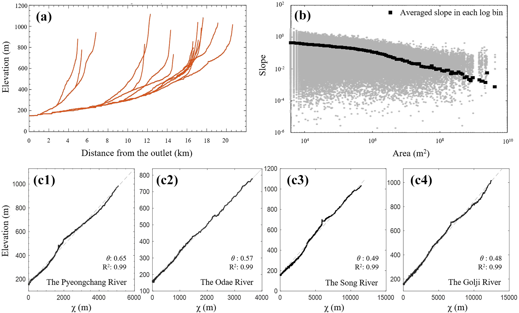
Stream longitudinal profiles of all studied stream branches (Figure 10a), slope-area scatter plot in the log-log scale (Figure 10b), in which a black square (▪) is an averaged value for raw slope data (•) in a log-bin for an extent of drainage area, and chi-elevation plots for the four longest branches which are likely to preserve the long history of transient knickzone evolution responding to the orogeny of the TMR (Figures 10c 1-4). Note that the interpretation of a transition in the slope-area curve around 10⁶ m² in Figure 10b should be undertaken with caution, which differentiates the slope-area relation into two regions and thus looks like a knickzone. However, it does indicate a transition in dominant erosion processes from colluvial channel to bedrock channel segments, which is a commonly observed feature in the slope-area relation of the landscape in steady-state (Montgomery, 2001). The thick black lines in Figures 10c 1-4 are chi-elevation plots based on Equations (5a) and (5b), the thin grey dash lines are the best linear fits with the optimal θ value, which is determined to maximize the linearity of the relation between chi and elevation of each profile. Thus, the higher linearity of chi-elevation plots, the larger R ² value.

4.3 Duration of transient knickzone migration

The absence of transient knickzones in the present landscape means that sufficient time has passed since the last active tectonic event. We can reason that transient knickzones formed by the tectonic event have propagated headward up to stream heads and disappeared. Knickzones might diminish as they migrate through different rock types (Crosby and Whipple, 2006), which could mask a signal of landscape transience. However, the heavy linearity in the slope-area relation and the chi-elevation plots for the studied rivers (Figure 10) suggests that even the upstream sections of the identified knickzones are indeed graded, thus confirming that the transient knickzones relevant to the growth of the TMR had transferred up to the watershed boundary. Hence, the entire study catchment had already been adjusted by this migration of the transient knickzones relevant to the past orogenic activity. Since then, it has reached a quasi-equilibrium state.

From this perspective, calculating a propagation period of each transient knickzone from the outlet to its stream head allows us to estimate the minimum age of the last enhanced tectonic activity that triggered the formation of the transient knickzone. Using equation (9), we calculated the migration periods of transient knickzones along the four longest surveyed branches, which thus might have the longest periods of knickzone migration (Table 3). As the study catchment was verified as quasi-steady-state, U in equation (9) was replaced with the incision rates of the study catchment from previous studies (Byun et al., 2015; Lee, 2009; Yoon et al., 2007). Since we assumed that knickzone propagation initiates at the catchment outlet and ends at the channel head, 0 was put into x_k in equation (9). Such knickzone initiation is reasonable because, given the topography across the middle of the peninsula, knickzone formation triggered by the TMR orogeny is considered to begin from the west coastline, that is, the outlet of the Han River (• in Figure 1b).

Table 3.

Estimated periods for the migration of a potential transient knickzone along the four longest stream branches in the study catchment, which are the same branches selected for the chi-elevation analysis. Note that the estimates depend on the uplift rate data of the study catchment.

Uplift rate in Equation (9) (mm/yr)	Migration time from the outlet to a head of each stream branch (yr)
Uplift rate in Equation (9) (mm/yr)	Pyeongchang River (PC)	Odae River (OD)	Song River (SC)	Golji River (GJ)
0.26^a	5,122,222	4,768,538	4,493,109	4,506,341
0.18^b	7,842,218	7,300,721	6,879,034	6,899,293
0.13^c	10,599,059	9,867,205	9,297,278	9,324,659

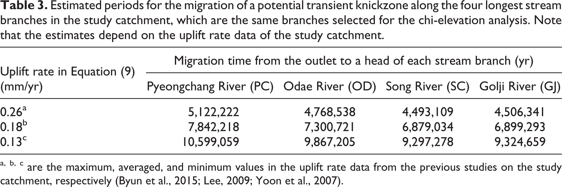
^a, ^b, ^c are the maximum, averaged, and minimum values in the uplift rate data from the previous studies on the study catchment, respectively (Byun et al., 2015; Lee, 2009; Yoon et al., 2007).

According to our estimation, the longest migration period of a transient knickzone is 5.12 Myr under a rapid uplift scenario of U=0.269 mm/yr based on the optically stimulated luminescence data (Lee, 2009). In a slower uplift scenario of U=0.130 mm/yr based on the cosmogenic radionuclides data (Byun et al., 2015), the longest migration period is 10.60 Myr. These times are the minimum age of the last period of accelerated uplift for the two scenarios. Thus, depending on U, the TMR orogeny dates back at least to 5.1 to 10.6 Myr ago. Considering the length of the examined course that is about one-fifth of that of the whole Han River (Figure 1b), through which the plausible transient knickzones relevant to the TMR formation would have propagated, the TMR orogeny would date back further.

Our estimate of transient knickzone duration within the study catchment has the same meaning as the response time of the entire study catchment to a past tectonic perturbation. Whipple (2001) proposed a fluvial response time T_r for an entire stream profile to be steepened following an enhanced tectonic forcing and to approach an equilibrium form, which is shown as

T_{r} = β K^{- 1 / n} U_{i}^{1 / n - 1} (f_{U}^{1 / n} - 1) (f_{U} - 1),

where $β = k_{a}^{- m / n} {(1 - h m / n)}^{- 1} (L^{1 - h m / n} - x_{c}^{1 - h m / n})$ = a purely geometric term; k_a and h = the inverse Hack coefficient and exponent (A = k_ax^h ), respectively; K = the erosion coefficient for an entire stream profile; U_i = the initial rock uplift rate; and f_u = U_i / U_f = the ratio of U_i to the final uplift rate U_f .

To validate the estimated transient knickzone duration, we calculated the response time of the study catchment using equation (10). The calculated response time for one of the longest studied branches in the study catchment, the Odae River (OD), was in the range between 4.16 and 9.35 Myr, depending on U_f and n (n = 2.6±0.4; Harel et al., 2016) (Supplementary Table 1). This result is similar to the estimated transient knickzone durations, thus demonstrating the reliability of our estimation.

V Discussion: development process of the coastal mountain range

The absence of transient knickzones and the heavy linearity in the slope-area relation and chi-elevation plots allow us to suggest that the study catchment is not experiencing any enhanced tectonic forcing but has sustained a topographic quasi-equilibrium state since the last accelerated tectonic activity. The incision rate data from previous studies (Byun et al., 2015; Lee, 2009;Yoon et al., 2007) also supports that the study catchment had already been adjusted through knickzone migration and has been in a quasi-equilibrium state.

In general, a drainage basin with transient knickzones shows a large difference in denudation rates between the upstream and downstream areas separated by transient knickzones. For example, Weissel and Seidl (1998) reported at least 25 times greater erosion rates at the downstream area of knickpoint (0.101 to 0.155 mm/yr) than the upstream plateau surface (0.003 to 0.004 mm/yr) in New South Wales, Australia. However, the bedrock incision rate at the uppermost plateau region in the study catchment obtained by the cosmogenic radionuclides technique (0.13±0.03 mm/yr, close to No. 13 knickzone in Figure 5; Byun et al., 2015) is not very distinguishable from those over the downstream regions of the studied stream branches: the incision rate for the downstream areas of the Golji River was in the range of 0.13 to 0.16 mm/yr estimated based on the chronology of river terraces (GJ in Figure 5; Yoon et al., 2007) and that for the downstream areas of the Odae River was in the range of 0.205 to 0.269 mm/yr measured by the optically stimulated luminescence dating method (OD in Figure 5; Lee, 2009). Such close incision rates between upstream and downstream regions show that the study catchment has been denuded at spatially similar rates, indicating that the study catchment is in a quasi-steady-state without landscape transience.

The quasi-steady-state study catchment could be used as critical evidence to invalidate the prevailed hypothesis that the TMR has formed progressively until the Late Quaternary (Kim, 1961, 1973; Yoshikawa, 1947). This hypothesis was built on the assumption that the low-relief surfaces observed at different altitudes across the middle part of the Korean Peninsula are denudation surfaces, each of which had formed through base-level lowering (or enhanced tectonic uplift) and subsequent long-term erosion. If this assumption is correct, the study catchment should have several transient signals at different altitudes. However, the few transient features we identified suggest that such low-relief surfaces are not transient but static, mainly due to lithological difference, and that the uplift scenario with multiple periods of accelerated uplift is not valid.

The migration period of transient knickzones through the study catchment was calculated in the range between 5.1 and 10.6 Myr. Although our estimate does not provide precise timing of the TMR orogeny, it gives a lower bound value. Moreover, the geomorphological evidence we provided demonstrates that the study catchment has been in a quasi-equilibrium state. These overall results help us to reconstruct the development of the coastal mountain range. Accelerated tectonic uplifts had built the coastal mountain range at least before 5.1 to 10.6 Myr ago. Since then, the coastal mountain range has sustained a topographic quasi-steady-state up to the present without landscape transience (Figure 11).

Figure 11.

The schematic sketch shows a progressive change of the longitudinal profile of the Han River to an accelerated tectonic uplift. Note that the dashed line at the bottom is a paleo Han River profile before the accelerated uplift. The other upper dashed lines are the remaining upstream reaches, which have not yet been adjusted by the enhanced tectonic forcing. The abrupt change points between the steepened downstream and upstream reaches on the profile are migrating transient knickzones.

The estimated migration period of transient knickzones of at least 5.1 Myr is interesting because it does not concede any tectonic forcing nearly since the Pliocene (2.6 to 5.3 Myr ago). It thus also rejects the prevalent hypothesis of long-lasting and progressive TMR development until the Late Quaternary. Such inconsistency with the long-lasting formation hypothesis may arise from an inaccurately determined depositional age of the Tertiary sedimentary rocks on the eastern side of the TMR (i.e. the Bukpyeong Formation), which are the direct results from the TMR orogeny and have been known to date back to the Pliocene (Choi and Bong, 1986; Yu, 1971). This relatively young age might have laid the foundation for the long-lasting TMR formation hypothesis. However, a recent study based on fauna records (i.e. the platacanthomyine rodent Neocometes, instead of pollen and diatoms) articulated that the age of the Bukpyeong Formation is constrained to the Early to Middle Miocene (15 to 18 Myr ago) (Lee and Jacobs, 2010). If this is correct, the formation of the coastal mountain range could date back further, at least to the Early Miocene. In that case, the hypothesis of the intensive uplift during the Early Miocene becomes more persuasive.

In addition, the estimated migration period of the transient knickzones provides an insight into the mechanism for the occurrence of high topography along the East Sea. Our estimation indicates that an accelerated tectonic uplift has not occurred at least since 5.1 Myr ago. Therefore, with the study catchment verified as a quasi-equilibrium state, post-extension uplift processes including flexural isostatic rebounds would not have made sufficient contribution to the net growth of the coastal mountain range but maintained the current form of the coastal mountain range. Presumably, the development up to the current form of the coastal mountain range is primarily associated with the tectonic processes that are directly related to the back-arc basin extension creating of the East Sea, such as thermally driven uplift due to lateral conduction of high heat from a ridge spreading site (e.g. Buck, 1986), and regional upward flexure due to thinning of the lithosphere (e.g. Weissel and Karner, 1989).

VI Summary and conclusions

To better understand the history of the formation of the coastal mountain range in the Korean Peninsula, we analyzed the knickzones in a catchment over the coastal mountain range. Terrain analysis using DEM supplemented by field survey identified 18 knickzones within the study catchment. They turned out to originate from lithological difference, locally resistant substrate, and accumulation of coarse bed materials from a low-order steep tributary. Consequently, all identified knickzones were classified as stationary. The well-defined linearity shown in the slope-area and chi-elevation analyses confirmed that the study catchment does not contain any transient knickzone, thus implying that the mountain range has been in a quasi-steady-state since the last enhanced tectonic activity. The estimated migration periods for potential transient knickzones through the study catchment suggested that the last enhanced tectonic forcing dates back at least to 5.1 to 10.6 Myr ago.

According to these results, we conclude that the coastal mountain range had formed at least before 5.1 to 10.6 Myr ago, and, since then, it has been in a topographic quasi-equilibrium state up to the present. Therefore, the prevailing hypothesis of the long-lasting and progressive development of the coastal mountain range until the Late Quaternary, which assumes that the Korean Peninsula has been undergoing tectonic transience, comes across as invalid. With our results, as well as the recent discovery on the depositional age of the Tertiary sedimentary rock (15 to 18 Myr ago) (Lee and Jacobs, 2010), we lend weight to the hypothesis that the coastal mountain range was built mostly during the Early Miocene when the East Sea had opened. A further direction of our study will be to provide more geomorphological evidence for this possibility.

Supplemental material

Supplemental Material, Supplemental_material - The development process of the Korean coastal mountain range: Examination from spatial distribution of knickzones

Supplemental Material, Supplemental_material for The development process of the Korean coastal mountain range: Examination from spatial distribution of knickzones by Jongmin Byun and Kyungrock Paik in Progress in Physical Geography: Earth and Environment

Footnotes

Acknowledgements

The authors thank Youngchan Kim for helping with the field survey and Yeong Bae Seong for constructive comments at the early stage of this study. The authors also acknowledge helpful comments and suggestions from two anonymous reviewers and the editor, which enabled the manuscript to be improved substantially.

Declaration of conflicting interests

The author(s) declared no potential conflicts of interest with respect to the research, authorship, and/or publication of this article.

Funding

The author(s) disclosed receipt of the following financial support for the research, authorship, and/or publication of this article: Jongmin Byun was supported by the Ministry of Education of the Republic of Korea and the National Research Foundation of Korea (NRF-2018S1A5A8031058). Kyungrock Paik was supported by the NRF grant funded by the Korea government (Ministry of Science and ICT) (NRF-2018R1A2B2005772).

ORCID iDs

Jongmin Byun

Kyungrock Paik

Supplemental material

Supplemental material for this article is available online.

References

Beeson

McCoy

Keen-Zebert

(2017) Geometric disequilibrium of river basins produces long-lived transient landscapes. Earth and Planetary Science Letters 475: 34–43.

Berlin

Anderson

(2007) Modeling of knickpoint retreat on the Roan Plateau, western Colorado. Journal of Geophysical Research 112: F03S06.

Buck

(1986) Small-scale convection induced by passive rifting: The cause for uplift of rift shoulders. Earth and Planetary Science Letters 77(3–4): 362–372.

Byun

Seong

(2015) An algorithm to extract more accurate stream longitudinal profiles from unfilled DEMs. Geomorphology 242: 38–48.

Byun

Heimsath

Seong

, et al. (2015) Erosion of a high-altitude, low-relief area on the Korean Peninsula: Implications for its development processes and evolution. Earth Surface Processes and Landforms 40(13): 1730–1745.

Cho

Min

Kim

(2018) Geology of the 2018 Winter Olympic site, Pyeongchang, Korea. International Geology Review 60(3): 267–287.

Choi

Bong

(1986) Neogene palynomorphs from lignite beds of Bugpyeong and Yeonghae areas, Korea. Journal of the Paleontological Society of Korea 2(1): 1–17.

Choi

Lee

(2007) The correlation of the last interglacial terraces of the southwestern coast with those of the eastern and western coasts of the Korean Peninsula. Journal of the Korean Geomorphological Association 14(3): 15–26 (in Korean with English abstract).

Choi

Seong

Jung

, et al. (2012) Using cosmogenic ¹⁰Be dating to unravel the antiquity of a rocky shore platform on the west coast of Korea. Journal of Coastal Research 28(3): 641–657.

10.

Crosby

Whipple

(2006) Knickpoint initiation and distribution within fluvial networks: 236 waterfalls in the Waipaoa River, North Island, New Zealand. Geomorphology 82: 16–38.

11.

Flint

(1974) Stream gradient as a function of order, magnitude, and discharge. Water Resources Research 10: 969–973.

12.

Gilchrist

Summerfield

(1990) Differential denudation and flexural isostasy in formation of rifted-margin upwarps. Nature 346: 739–742.

13.

Hanks

Webb

(2006) Effects of tributary debris on the longitudinal profile of the Colorado River in Grand Canyon. Journal of Geophysical Research: Earth Surface 111(F2): F02020.

14.

Harel

M-A

Mudd

Attal

(2016) Global analysis of the stream power law parameters based on worldwide ¹⁰Be denudation rates. Geomorphology 268: 184–196.

15.

Hayakawa

Oguchi

(2006) DEM-based identification of fluvial knickzones and its application to Japanese mountain rivers. Geomorphology 78: 90–106.

16.

Hayakawa

Oguchi

(2009) GIS analysis of fluvial knickzone distribution in Japanese mountain watersheds. Geomorphology 111: 27–37.

17.

Hayashida

Fukui

Torii

(1991) Paleomagnetism of the Early Miocene Kani Group in southwest Japan and its implication for the opening of the Japan Sea. Geophysical Research Letters 18: 1095–1098.

18.

Jolivet

Tamaki

(1992) Neogene kinematics in the Japan Sea region and volcanic activity of the northeast Japan Arc. Proceedings of the Ocean Drilling Program, Scientific Results, Legs 127/128, 1311–1331.

19.

Jolivet

Tamaki

Fournier

(1994) Japan Sea, opening history and mechanism: A synthesis. Journal of Geophysical Research 99: 22237–22259.

20.

Kim

H-J

Lee

Jou

H-T

, et al. (2007) Evolution of the eastern margin of Korea: Constraints on the opening of the East Sea (Japan Sea). Tectonophysics 436: 37–55.

21.

Kim

S-H

(1961) Topographical development of the Central Korea. Seoul University Journal 10: 111–123 (in Korean with English abstract).

22.

Kim

S-H

(1973) Geomorphic studies of the erosion surfaces in Central Korea. Seoul University Journal 21: 85–115 (in Korean with English abstract).

23.

Kim

S-H

(1980) The introduction of the landscape formation and development of the Korean Peninsula. The Geographical Journal of Korea 5: 1–15 (in Korean).

24.

Kim

Y-S

Jin

Choi

W-H

, et al. (2011) Understanding of active faults: A review for recent researches. Journal of the Geological Society of Korea 47(6): 723–752 (in Korean with English abstract).

25.

Kirby

Whipple

(2012) Expression of active tectonics in erosional landscapes. Journal of Structural Geology 44: 54–75.

26.

Kwon

. (2000) Mountain ranges of Korea. Journal of the Korean Geographical Society 35(3): 389–400 (in Korean with English abstract).

27.

Lallemand

Jolivet

(1986) Japan Sea: A pull-apart basin? Earth and Planetary Science Letters 76: 375–389.

28.

Lee

G-R

(2009) Properties of channel and evolutions of fluvial terraces in Odae River. Journal of the Korean Geographical Society 44: 224–239 (in Korean with English abstract).

29.

Lee

Y-N

Jacobs

(2010) The platacanthomyine rodent Neocometes from the Miocene of South Korea and its paleobiogeographical implications. Acta Palaeontologica Polonica 55(4): 581–586.

30.

Montgomery

(2001) Slope distributions, threshold hillslopes, and steady-state topography. American Journal of Science 30: 432–454.

31.

National Emergency Management Agency (2011) The current status in the research of active faults in the Korean Peninsula. The Magazine of the Korean Society of Hazard Mitigation 11(1): 117–123 (in Korean).

32.

Niemann

Gasparini

Tucker

, et al. (2001) A quantitative evaluation of Playfair’s law and its use in testing long-term stream erosion models. Earth Surface Processes and Landforms 26: 1317–1332.

33.

Ortega

Wohl

Livers

(2013) Waterfalls on the eastern side of Rocky Mountain National Park, Colorado, USA. Geomorphology 198: 37–44.

34.

Otofuji

Y-I

(1996) Large tectonic movement of the Japan Arc in late Cenozoic times inferred from paleomagnetism: Review and synthesis. Island Arc 5: 229–249.

35.

Otofuji

Y-I

Matsuda

Nohda

(1985) Opening mode of the Japan Sea inferred from the palaeomagnetism of the Japan Arc. Nature 317: 603–604.

36.

Park

Ree

J-H

Yoo

S-H

(2006) Fault slip analysis of Quaternary faults in southeastern Korea. Gondwana Research 9: 118–125.

37.

Pechlivanidou

Cowie

Duclaux

, et al. (2019) Tipping the balance: Shifts in sediment production in an active rift setting. Geology 47: 259–262.

38.

Perron

Royden

(2013) An integral approach to bedrock river profile analysis. Earth Surface Processes and Landforms 38: 570–576.

39.

Phillips

McCormack

Duan

, et al. (2010) Origin and interpretation of knickpoints in the Big South Fork River basin, Kentucky-Tennessee. Geomorphology 114: 188–198.

40.

Snyder

Whipple

Tucker

, et al. (2000) Landscape response to tectonic forcing: Digital elevation model analysis of stream profiles in the Mendocino triple junction region, Northern California. Bulletin of the Geological Society of America 112: 1250–1263.

41.

Song

U-G

(1998) Geomorphic development of river terrace and meander cut-off in the Donggang. Journal of the Geomorphological Association of Korea 5(2): 109–130 (in Korean with English abstract).

42.

Tamaki

Suyehiro

Allan

, et al. (1992) Tectonic synthesis and implications of Japan Sea ODP drilling. Proceedings of the Ocean Drilling Program, Scientific Results, Legs 127/128, 1333–1348.

43.

Wang

Zhang

Zheng

, et al. (2017) How a stationary knickpoint is sustained: New insights into the formation of the deep Yarlung Tsangpo Gorge. Geomorphology 285: 28–43.

44.

Weissel

Karner

(1989) Flexural uplift of rift flanks due to mechanical unloading of the lithosphere during extension. Journal of Geophysical Research 941: 13919–13950.

45.

Weissel

Seidl

(1998) Inland propagation of erosional escarpments and river profile evolution across the southeast Australian passive continental margin. In: Tinkler

Wohl

(eds) Rivers over Rock: Fluvial Processes in Bedrock Channels. Washington, DC: American Geophysical Union, 189–206.

46.

Whipple

(2001) Fluvial landscape response time: How plausible is steady-state denudation? American Journal of Science 301: 313–325.

47.

Whipple

Tucker

(1999) Dynamics of the stream-power river incision model: Implications for height limits of mountain ranges, landscape response timescales, and research needs. Journal of Geophysical Research B: Solid Earth 104: 17661–17674.

48.

Whipple

DiBiase

Ouimet

, et al. (2017) Preservation or piracy: Diagnosing low-relief, high-elevation surface formation mechanisms. Geology 45: 91–94.

49.

Whipple

Hancock

Anderson

(2000) River incision into bedrock: Mechanics and relative efficacy of plucking, abrasion, and cavitation. Bulletin of the Geological Society of America 112: 490–503.

50.

Whittaker

Boulton

(2012) Tectonic and climatic controls on knickpoint retreat rates and landscape response times. Journal of Geophysical Research: Earth Surface 117. DOI: 10.1029/2011JF002157

51.

Willgoose

(1994) A physical explanation for an observed area-slope-elevation relationship for catchments with declining relief. Water Resources Research 30: 151–159.

52.

Wobus

Whipple

Kirby

, et al. (2006) Tectonics from topography: Procedures, promise, and pitfalls. Geological Society of America Special Paper 398: 55–74.

53.

Yoon

Chough

(1995) Regional strike slip in the eastern continental margin of Korea and its tectonic implications for the evolution of Ulleung Basin, East Sea (Sea of Japan). Geological Society of America Bulletin 107: 83–97.

54.

Yoon

Sohn

Chough

(2014) Tectonic, sedimentary, and volcanic evolution of a back-arc basin in the East Sea (Sea of Japan). Marine Geology 352: 70–88.

55.

Yoon

S-O

Hwang

Lee

G-R

(2007) Geomorphic evolution of fluvial terraces at Yeongdong·Yeongseo streams in Gangwon Province, Korea. Journal of the Korean Geographical Society 42(3): 388–404 (in Korean with English abstract).

56.

Yoshikawa

(1947) The geomorphic history of Central Korea. Journal of the Geological Society of Japan 53(616): 28–32 (in Japanese).

57.

(1971) The Tertiary fossil pollens and diatoms from Bukpyeong, Korea. Bulletin of the Geological Survey of Korea 13: 449–484 (in Korean with English abstract).

Supplementary Material

Please find the following supplemental material available below.

For Open Access articles published under a Creative Commons License, all supplemental material carries the same license as the article it is associated with.

For non-Open Access articles published, all supplemental material carries a non-exclusive license, and permission requests for re-use of supplemental material or any part of supplemental material shall be sent directly to the copyright owner as specified in the copyright notice associated with the article.

0.00 MB

0.03 MB