Morphodynamic modelling of dryland non-perennial riverscapes,with implications for environmental water allocation

Abstract

Reach-scale river restoration or environmental water allocation (EWA) exercises typically address the magnitude and temporal dynamics (frequency, duration, timing, rate of change) of flows required to sustain desirable ecological conditions along a river. The role of geomorphology in this process is to broaden the gaze beyond flows to consider larger and longer-term interactions between valley lithological structure, and the feed and fate of flow-sediment mixtures. This paper proposes the integration of numerical morphodynamic modelling in evaluations of environmental water requirements for non-perennial riverscapes (channel–riparian–floodplain environments). The paper presents a methodological framework, and proof of concept case study from the Touws River, South Africa, for the application of morphodynamic modelling in EWA. The paper illustrates operational approaches to modelling the complexity of dryland mixed bedrock-alluvial (and mixed-load) riverscapes with highly variable non-perennial flow regimes, including an approach to generating initial bed conditions for numerical experiments by ‘morphodynamic spin-up’, and approaches to synthesising and presenting numerical experiment output in the form of a dynamic range of potential variability in metrics of physical habitat suitability and diversity, and disturbance/renewal regimes. Such efforts can assist in enhancing field observations and testing field-based hypotheses of flow-sediment regime–physical habitat associations, extending the timescales of analysis beyond field observation, and constraining uncertainty about the dynamic range of variability in responses to predicted future flow-sediment regime modifications. Further research is needed to develop growth models appropriate for key non-perennial river vegetation types, to support biomorphodynamic modelling of geomorphology–vegetation interactions, and to determine or predict appropriate inlet sediment concentrations for historical and future modification scenarios.

Keywords

Fluvial geomorphology and ecology eco-geomorphology biogeomorphology environmental flows intermittent rivers and ephemeral streams

I Introduction

Reach-scale river restoration or environmental water allocation (EWA) exercises typically address the magnitude and temporal dynamics (frequency, duration, timing, rate of change) of flows required to sustain desirable ecological conditions along a river (Dyson et al., 2003; Tharme, 2003). The role of geomorphology in this process is to broaden the gaze beyond flows to consider larger and longer-term interactions between valley lithological structure, and the feed and fate of flow-sediment mixtures (Meitzen et al., 2013; Rowntree, 2013; Thoms and Sheldon, 2002). From an ecological perspective, fluvial geomorphology represents both a blank habitat ‘canvas’ and a rough disturbance/renewal/resource-dispersal ‘brush’ for river ecosystem structure and function (Brierley and Fryirs, 2005; Dollar et al., 2007; Thoms, 2006; Thoms and Parsons, 2002; Ward et al., 2002). In combination with flow variability and the physico-chemistry of water and sediment, geomorphic features set the physical template of river habitat (Brierley and Fryirs, 2005; Petts and Amoros, 1996; Vannote et al., 1980). At relatively small scales of space and time, the ‘blank canvas’ of geomorphic units and substrate influences flow velocities, turbulence, inundation depths, and boundary permeability, which shapes biotic assemblages in a river (Frissell et al., 1986; Padmore, 1998; Wadeson and Rowntree, 1998). Over longer timescales, geomorphic resetting events, such as large floods, influence channel-bar patterning, local elevation gradients and edaphic transitions, inundation-frequency surface distributions, and spatial sediment sorting. These characteristics have strong influences on ecological succession and renewal (Heritage et al., 2004; Rountree et al., 2000; Thoms, 2006; Thorp et al., 2006).

In the case of non-perennial rivers, the high spatial and temporal variability in water availability and sediment dispersal processes poses several challenges to sustainable riverscape management in general (Datry et al., 2017), and EWA in particular (Seaman et al., 2010, 2013, 2016). For example, non-perennial river flows with high temporal variability interact with other features of the biophysical setting to generate a diverse and sometimes distinctive array of fluvial styles at multiple scales of space and time (Dollar and Rowntree, 2003; Jaeger et al., 2017; Rountree et al., 2001; Thoms and Parsons, 2002; Tooth, 2012, 2013). However, the necessary conditions for the development of particular physical habitat assemblages are not well understood. This makes it difficult to predict flow conditions (and sediment supply; Wohl et al., 2015) required within a given valley structural setting to conserve a particular habitat condition (e.g. Acreman et al., 2014). An integration of field, laboratory, and numerical model-based enquiry has the potential to improve prediction of physical habitat assemblages (Jaeger et al., 2017; Kleinhans, 2010; Milan et al., 2018a; Poff, 2018).

The management of non-perennial riverscapes is further complicated by the need to recognise that the desired condition is neither singular, nor static in its characteristics, processes, and behaviour (Du Preez and Rowntree, 2006; Rowntree, 2013). Rather, there is a dynamic range of variability in physical habitat responses to environmental forcing arising from flow modifications by water resource developments, climatic variability, or climate change (Heritage et al., 1997; Hooke, 2016; Meitzen et al., 2013; Milan et al., 2018a). It is seldom possible to physically observe the dynamic range of ‘natural’ variability (DRNV) in riverscape system states and successional trajectories, over a multi-decadal time period, at landscape scale (Frissell and Bayles, 1996; Landres et al., 1999). This is especially challenging for non-perennial rivers, which are characterised by long periods of low or no flow, punctuated by cyclical or unpredictably episodic floods (Puckridge et al., 1998; Rountree et al., 2001; Thoms and Delong, 2018; Uys and O’Keeffe, 1997). For most riverscapes, the scale of past and current human modifications precludes accurate characterisation of a pre-disturbance DRNV as a reference condition (Brierley and Fryirs, 2005; Seaman et al., 2010; Ward et al., 2001). The potential future conditions of alteration associated with water resource development, future boundary conditions, and the biotic and social-ecological response are similarly difficult to predict. However, there are two broad approaches that may be applied to gain insight into possible responses of physical habitats to flow regime modifications.

One approach is to employ inductive and abductive ergodic reasoning (space-for-time substitution (Fryirs et al., 2012; Ward et al., 1999) to investigate a historical range of variability as a basis for understanding system responses to changes in flux boundary conditions involving flow (Poff, 2018; Poff et al., 1997; Puckridge et al., 1998), sediment (Wohl et al., 2015), and wood (Wohl et al., 2019) regimes. Allied to this approach, one may propose a future dynamic range of potential variability based on empirical conceptual modelling informed by time-series image analysis, field survey, and geochronology (e.g. Heritage et al., 1997; Osterkamp and Hupp, 2010; Thoms and Sheldon, 2002), riverscape digital elevation modelling (e.g. Brown et al., 2014, 2016; Hillier et al., 2015), or classification-based river trajectory reasoning (Brierley and Fryirs, 2005; Fryirs and Brierley, 2013). An alternative but complimentary approach is to model a dynamic range of potential variability (DRPVm) in physical geomorphological habitat, using numerical experiments that illustrate the physical habitat responses to predicted changes in domain and flux boundary conditions (e.g. Arboleda et al., 2010; Bertoldi et al., 2014; Brown and Pasternack, 2019; Milan et al., 2018b, 2020).

This paper proposes the application of numerical morphodynamic modelling in the evaluation of linkages between flow regime modifications and physical geomorphological habitats of non-perennial riverscapes. The paper presents a methodological numerical modelling framework, and proof of concept case study from the Touws River, South Africa, and considers implications for the incorporation of modelling outputs in EWA exercises. The paper does not pit empirical-conceptual and numerical modelling approaches against one another, but rather argues for the incorporation of morphodynamic modelling where this can add value to the EWA process, especially in ‘flashy’ systems with high morphodynamic sensitivity (Brunsden and Thornes, 1979; Knighton and Nanson, 1997; Tooth, 2013). An integration of all available insights from all available approaches is most likely to lead to the development of mature morphodynamic explanations of key controls and necessary conditions for elements and mosaics of physical habitats (Kleinhans, 2010).

II Geomorphology as a component of non-perennial riverscape habitat

At the reach scale, a number of geomorphic features may be identified that have particular habitat significance for non-perennial river biota (see examples from the Prins and Touws Rivers in South Africa in Figure 1). First, there are longitudinally concave features such as pools or waterholes (Figure 1(a)–(d)) that are able to retain water and serve as key aquatic refugia when flows cease (Biggs et al., 2017; Bunn et al., 2006; Hamilton et al., 2005; Jaeger et al., 2017; Seaman et al., 2010; Sheldon et al., 2010). Figure 1(a)–(d) shows examples of pools located adjacent to rock outcrops, the most common pool type within the rivers shown, and also the deepest and most persistent type (Hattingh, 2020). Smaller and less persistent depressions are located adjacent to debris bars that form in association with Vachellia karroo tree stems or debris piles (shown in Figure 1(g), (h)). The problem of pool persistence (Reid et al., 2017; Rossouw et al., 2005; Seaman et al., 2010) is one that requires the equal attention of hydrologists, hydrogeologists (Boulton et al., 2017), and geomorphologists. The decadal-scale morphodynamics of a riverscape determine why, where, and how depressions form (Heritage et al., 1999; Knighton and Nanson, 1994, 2000), depression depth (with implications for losses to evaporation; Bunn et al., 2006; Hamilton et al., 2005), and depression bed sediment thickness (with implications for sub-bed storage capacity and losses to infiltration; Jaeger et al., 2017).

Figure 1.

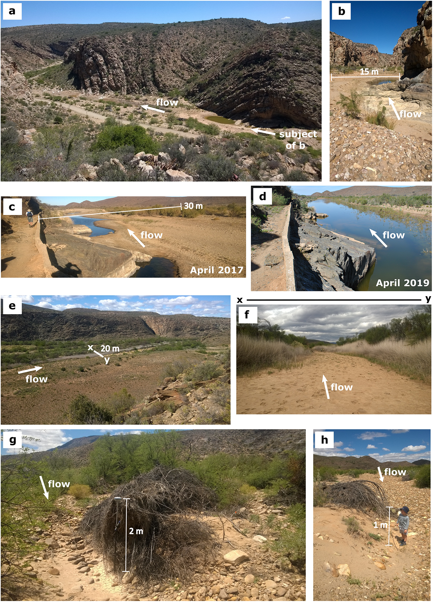
Examples of geomorphic and biogeomorphic features/elements of physical habitat that play an important role in the ecology of dryland non-perennial riverscapes. Images are from the Prins and Touws rivers in the Klein Karoo, Western Cape, South Africa. Large pools (a-d) are located in close association with bedrock outcrops. Reed beds (e, f) occur where there is sustained saturation of the root zone. Forced mid-channel bars occur in the lee of Vachellia karroo stems and/or debris piles.

Second, stand-forming hydrophytic vegetation that colonises the margins of depressions (e.g. Phragmites australis reed beds; Figure 1(e), (f)), or in some settings is able to spread through rhizome networks to cover extensive areas of the valley floor, provides geomorphologically transient wetland habitat (Kotschy et al., 2000; Makhonco, 2019). During long no-flow periods the rivers shown in Figure 1 behave as networks of relatively isolated wetlands within a mosaic of sparsely vegetated dry sediment features (Grenfell et al., 2019). There is a need for an improved understanding of how spatial and temporal variation in aquatic–wetland linkages (Leigh et al., 2010) and aquatic–terrestrial linkages (Leigh et al., 2016) affect physical habitats in non-perennial riverscapes. Riparian vegetation is a dynamic driver of riverscape morphodynamics (Bertoldi et al., 2014; Van Oorschot et al., 2016).

Third, there are longitudinally convex features such as sediment bars (Figure 1(g), (h)) that determine the steepness of terrestrial to wetland or aquatic transitions, and the nature of topographic diversity, which interact with water availability and biogeochemistry to define species tolerance continua or thresholds of habitat suitability and diversity (Scown et al., 2016; Thorp et al., 2006). Understanding associations between fluvial style and topographic or substrate complexity (e.g. Brierley and Fryirs, 2005; Eze and Knight, 2018; Scown et al., 2016), and how these associations are shaped by decadal-scale morphodynamics (e.g. alternation of physical states; Rountree et al., 2001; Rowntree, 2013), is invaluable to enhancing the predictive power of EWA methodologies. Forced mid-channel bars (sensu Brierley and Fryirs, 2005) that form in the lee of debris piles or tree stems are the most common bar type in the rivers shown in Figure 1(g), (h).

Finally, greater emphasis should be placed on dispersal processes that define such notions as the ‘biogeochemical heartbeat’ of non-perennial rivers, where the movement and processing of sediment and associated biogeochemically reactive elements (BREs) is dynamically pulsed over decadal and longer timescales (Von Schiller et al., 2017: 135–136). The nature of BRE dispersal and cycling as described is consistent with the variable nature of hydrological forcing, and aligned with geomorphological descriptions of non-perennial rivers as especially jerky conveyor belts for sediment (in concept, after Ferguson, 1981: 90), due to their high degree of longitudinal dis-connectivity (Brierley and Fryirs, 2005; Burchsted et al., 2014), and transport-limited character (Milliman and Farnsworth, 2011). The dispersal processes and exchange fluxes of water–sediment mixtures and associated BREs are important determinants of habitat suitability and resource availability for resident biota (Von Schiller et al., 2017).

Given the above, there is a need to develop indices that capture the DRPV in riverscape morphodynamics, the hydrologically coupled influence of morphodynamics on flow/inundation/saturation regimes for key physical habitat features and processes, and the broader links to neighbouring wetland (Leigh et al., 2010) and terrestrial (Leigh et al., 2016) environments. The incorporation of physical habitat insights into widely applied EWA decision support systems such as DRIFT (King et al., 2003) or DRIFT-ARID (Seaman et al., 2013, 2016) requires expressions of the dynamic range of variability in hydrological, geomorphological, and physico-chemical attributes in a form that is useful to ecologists, such that clear links may be drawn to the biotic or social-ecological outcomes of changes in these driving forces (King and Brown, 2006; Seaman et al., 2010). The framework and case study presented hereafter aims to illustrate the value of morphodynamic modelling in this endeavour.

III Methodological framework for the application of morphodynamic modelling in EWA

Several developments in river morphodynamic modelling are relevant to and have informed the approach demonstrated in this paper (see Brown and Pasternack, 2019, for a full review). These developments were drawn from previous studies that i) highlighted the importance of representing discharge variability in evaluating the effects of river engineering works (Huthoff et al., 2010), and of representing sediment heterogeneity in replicating channel-bar features and patterns (De Almeida and Rodríguez, 2011; Singh et al., 2017); ii) resolved the physical and biophysical conditions necessary for the formation and maintenance of, for example, reach-scale riverscape channel-floodplain patterns (e.g. Murray and Paola, 1994; Nicholas, 2013), pool-riffle sequences in single-thread rivers (De Almeida and Rodríguez, 2011, 2012), or island formation in variable-flow mixed bedrock-alluvial anabranching rivers (Milan et al., 2018b, 2020); and iii) attempted to reconstruct historical (Arboleda et al., 2010) or predict future (Martínez-Fernández et al., 2018) riverscape environments based on predicted historical/future domain and flux boundary conditions.

The morphodynamic modelling approach demonstrated in this paper combines i) geospatial analysis of historical channel planform dynamics; ii) geospatial and field survey of proto-riverscape morphology, sediment, and roughness elements, for model domain setup and parameterisation, and evaluation of simulation output; and iii) analysis of river discharge data to define an inlet flow time-series and outlet stage–discharge relation as flux (mass/momentum) boundary conditions. The approach is illustrated conceptually in Figure 2, and follows the ‘morphodynamic canon’ of Ferguson (1981: 90), where ‘channels [and indeed riverscapes] are viewed as the outcome of a continuous struggle between the erosive potential of the river and the resistive forces of the valley-floor setting’. Forces of energy and resistance are integrated in a morphodynamic model, applied at riverscape-reach scale, through the definition of inlet and outlet flux boundary conditions, a valley form template (a boundary-fitted grid and initial morphology), and a valley composition template wherein elements of grain-, form-, and/or vegetation-related resistance are either represented explicitly or parameterised at sub-grid scale.

The integration of energy and resistance is operationalised within a morphodynamic model through the numerical routing of flow, computation of hydraulic properties across the domain, prediction of sediment transport, and associated morphological updating of the bed, which feeds back to inform subsequent hydraulic computations (Figure 2; ‘the morphodynamic lens’). A variety of physical riverscape attributes are stored for each output time-step in a simulation run, providing an image of the riverscape environment at different stages of development in response to flux boundary time-series forcing and morphodynamic interaction (Figure 2; ‘the image’). Spatio-temporal integration of all output time-step information in a composite DRPVm product provides insight into the DRPV in physical habitat for a given flux boundary time-series scenario (Figure 2; ‘the album’). Finally, the interpretation of the DRPVm by a multidisciplinary team provides one of several bases (King et al., 2003, 2008; Seaman et al., 2016; Thoms and Sheldon, 2002) for understanding biotic or social-ecological responses to the given flux boundary scenario.

Figure 2.

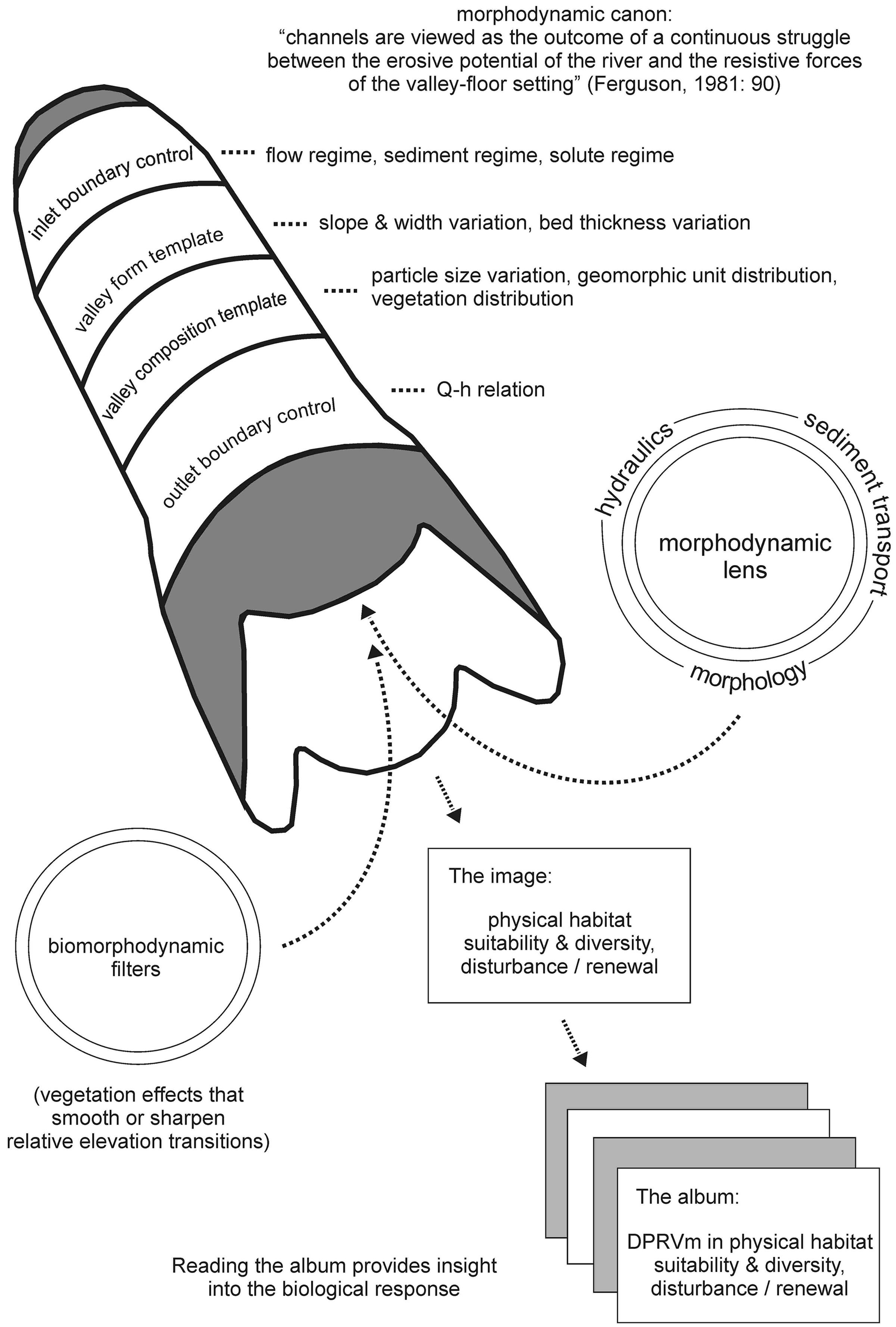
Conceptual framework for a morphodynamic modelling approach to understanding and constraining the dynamic range of potential variability (DRPVm) in physical habitat suitability and diversity, and disturbance/renewal regimes for scenarios of flow regime history or potential future modification. The phrase ‘dynamic range of variability’ is used to account for the full pattern of states and system trajectories possible within a given set of forcing conditions, rather than the pure biostatistics definition of the ‘range of variability’ based only on extreme-end states (after Frissell and Bayles, 1996; Frissell et al., 1997; Rhodes et al., 1994).

IV Proof of concept case study: Touws River at Plathuis, Western Cape, South Africa

An approximately 3.5-km-long reach of the Touws River near the town of Plathuis in the Klein Karoo, South Africa (Figure 3), was chosen as a proto-riverscape for model development due to the observed representation of a regionally pervasive valley form sequence (a laterally unconfined to partly confined transition). This location also benefited from its proximity to a Department of Water and Sanitation (DWS) gauging station (Okkerskraal; J1H018) with a multi-decadal (1982–2019) daily flow data record to inform model inlet flow time-series and outlet stage–discharge relations, as well as the availability of local rainfall observations spanning the period of DWS flow data, and was distant from major valley-spanning infrastructure such as road bridges, which would influence the dynamics of large flood events. There was also ease of access for fieldwork.

Figure 3.

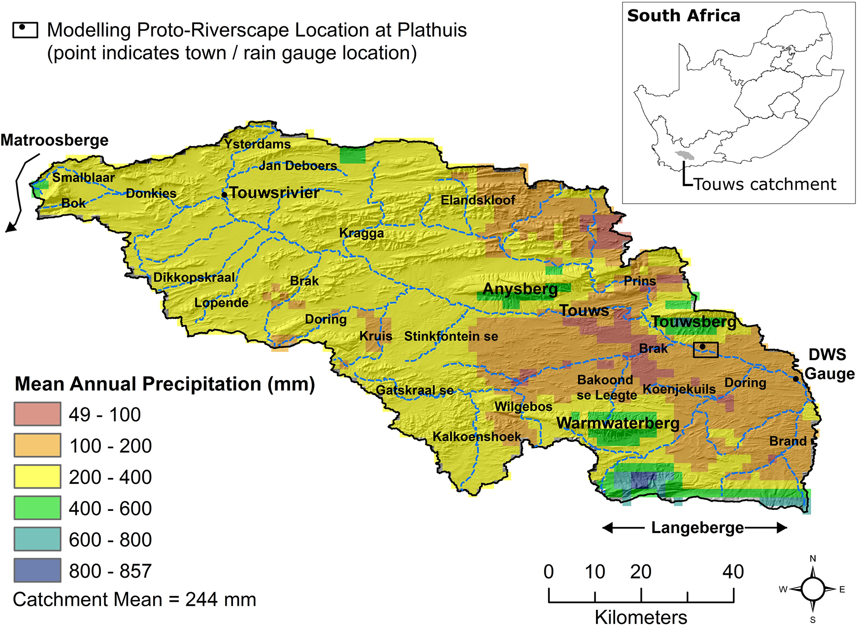
Site location in the context of regional physiography.

Empirical geospatial and field data were used to prepare a numerical morphodynamic model representing proto-riverscape conditions, and to evaluate model output. From an operational perspective, the data described above are often not available for many non-perennial rivers, hence the need for improving prediction of flows and sediment transport in ungauged basins (e.g. Heritage et al., 2019).

1 Regional setting and study site description

The name of the Touws River is thought to derive from the Nama tsao-s or ‘ash’, which may refer to a salt-tolerant plant common in the Klein Karoo (in Afrikaans, ‘asbosse’ or ash bushes; Caroxylon aphyllum, formerly Salsola aphylla), or more poignantly in the context of this research, to the colour of sediment-laden floodwaters (TANAP, 2019). The source of the Touws River lies upstream of the town of Touwsrivier (Figure 3). From here, the river flows south-east for ∼140 km to the confluence with the Groot River, which is downstream of the DWS gauging station (Figure 3). The catchment area up to the proto-riverscape site is 5763 km², and 5837 km² at the DWS gauging station.

The mean annual precipitation (MAP) for the overall catchment is 244 mm/year (Lynch and Schulze, 2007), and mean annual potential A-Pan evaporation (PE) is 2087 mm/year (Schulze and Maharaj, 2007), yielding a UNEP (1997) Aridity Index of 0.12 (arid). Spatial variation in MAP (Figure 3) and PE is high, with the proto-riverscape site at Plathuis characterised by a MAP of 155 mm/year (Lynch and Schulze, 2007), PE of 2253 mm/year (Schulze and Maharaj, 2007), and UNEP (1997) Aridity Index of 0.07 (arid). Vegetation of the upper catchment is dominated by Renosterveld of the Units FRs 6 (Matjiesfontein Shale Renosterveld) and FRs 7 (Montagu Shale Renosterveld), with small areas of Fynbos such as Units FFs 23 (North Swartberg Sandstone Fynbos) and FFs 24 (South Swartberg Sandstone Fynbos), varying with aspect, on sandstone relief such as Anysberg and Touwsberg (Mucina and Rutherford, 2006). The plains and low undulating hills of the middle to lower catchment are dominated by succulent and non-succulent shrubland of Unit SKv 8 (Western Little Karoo), with patches of Unit SKv 10 (Little Karoo Quartz Vygieveld) growing largely on soils weathered from quartz veins within mud-dominated lithologies (Mucina and Rutherford, 2006). The riverscape/riparian corridor of the lower Prins, leading into the Touws and downstream (including through the proto-riverscape site) to the confluence with the Groot River, comprises riverine thicket vegetation of Unit AZi 8 (Muscadel Riviere), which is dominated by Vachellia karroo, Caroxylon/Salsola spp. (Mucina and Rutherford, 2006), and, recently, by an emerging invasion of the alien Tamarix ramosissima (salt cedar). Muscadel Riviere vegetation is associated with a high mean annual temperature of 17.9°C, with summer temperatures sometimes exceeding 40°C (Mucina and Rutherford, 2006).

At the proto-riverscape site, the Touws River is a mixed bedrock-alluvial river with a bi-modal bed sediment composition, with peaks in D₅₀ at 47 mm (very coarse gravel, n = 22 sites × 100 clasts, Wolman Pebble Count) and 0.31 mm (medium sand, n = 29 sites, Mechanical Sieving) (Grootboom, 2019), and a complex channel morphology in profile and planform. Partly confined areas comprise a predominantly single-thread channel with a macro-channel/bedrock-abutting valley floor margin, and a nested inset channel marking the margins of large pools (Figure 4). The inset channel also impinges upon a bedrock valley margin in places where pools are located at outer bends in the valley/macro-channel course. The bed of the inset channel through pools is covered by a thin veneer of sandy-gravel above Adolphspoort Formation shale. Laterally unconfined areas comprise largely dual-thread wandering channels, with sediment thicknesses of 1 to 3 m (Grootboom, 2019), although channel thalwegs are still largely superimposed on the shale bedrock. The bar pattern is similarly nested, with macro-channel point bars forming inner bank margins of inset channels in partly confined areas, and large islands forming bank margins of inset channels in laterally unconfined areas, while superimposed upon these macro-bars is a set of smaller bar features that are almost entirely associated with leeward deposition of sediment behind thorn trees (Vachellia karroo) or thorn-wood debris piles (Grootboom, 2019; Figure 5). Such nested displays of macro/inset channels have been described for other dryland rivers with variable flow regimes (e.g. Heritage et al., 2001; Rountree et al., 2001; Rowntree, 2008; Thoms et al., 2006). The mixed bedrock-alluvial nature of the river poses certain challenges for morphodynamic modelling, which are discussed in Section IV.2 (‘Model preparation’).

Figure 4.

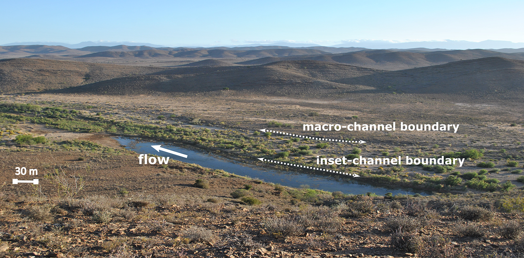
Oblique aerial view (oriented south-southeast) of a partly confined section of the proto-riverscape reach, showing the macro-channel and inset-channel boundaries. The image was captured on 9 December 2019 during a no-flow period. The pool pictured is at ∼60% of full capacity, retaining water from a flow in February 2019, a local 34 mm rainfall event in Oct 2019 (that produced no connecting flow response), and an unknown contribution of groundwater discharge.

2 Model preparation

The two-dimensional depth-averaged version of Delft3D (Deltares; version 4.03.01, fully validated commercial code) was used to model the morphodynamics of the proto-riverscape, and, in particular, to investigate variation in the morphodynamic response of the system to contrasting flow regime (inlet flow time-series) scenarios. This modelling system solves the two-dimensional depth-averaged form of the Navier–Stokes shallow water equations on a curvilinear finite-difference numerical grid, and has been validated for a range of hydrodynamic and morphodynamic applications (Gerritsen et al., 2008; Lesser et al., 2004). The model routes a specified inlet flow time-series through the grid in accordance with mass and momentum interactions between the hydraulic boundary conditions and a specified grid morphology, computes hydraulic properties across the model domain, and applies these hydraulic properties to compute sediment transport in each cell. This is followed by real-time, fully coupled morphological updating of the bed, such that the flow-routing computations at each time-step always ‘feel the effects’ of changes in morphology affected at the previous time-step. This is a significant advantage in the context of EWA, because it allows for the evaluation of a dynamic response in hydrogeomorphology (and derived attributes of physical habitat) to variation in flow, which cannot be achieved by imposing a variable water level on a fixed morphology (as in eco-hydraulic modelling; Gore et al., 2001; James and King, 2010). All simulations were run with equal hydrodynamic and morphodynamic computational time-steps (no morphological acceleration was applied, given the explicit focus on responses to a variable inlet flow time-series).

2.1 The model domain

A boundary-fitted orthogonal curvilinear grid was developed in the Delft3D RGFGRID software by importing splines that had been digitised in a geographic information system along the proto-riverscape valley floor margins, and across the inlet and outlet locations, from 0.5 m resolution orthorectified and georeferenced aerial photography captured in 2013. The grid was adjusted iteratively to ensure compliance with Delft3D quality criteria (Delft3D Modelling Guide, 2018) for orthogonality (<0.04), smoothness (<1.1), and aspect ratio (up to 5 for river applications where flows are primarily in the streamwise direction). Grid resolution was informed by the field dimensions of the inset channel (6–12 cells across the width of the 30–60 m inset channel, with a typical cell width of 5 m and typical aspect ratio of 3). A base domain morphology was developed in the Delft3D QUICKIN software using a point cloud derived from an ArcGIS Topo-to-Raster interpolation of 5 m contour elevation data (NGI, 2010). The grid and base morphology represent the macro-morphology of the riverscape domain in terms of valley width and longitudinal slope variation – the broad-scale valley form template (Figure 2) – and allow for morphodynamic adjustments to the form of the macro-channel/valley floor, inset channel, and the alluvial bars/islands/benches that define the macro/inset channel pattern.

This initial simplified morphological configuration was primed for subsequent numerical experiments by running an inlet flow time-series derived from the gauged historical flow record (see Section IV.2.3, ‘The inlet flow time-series’). At the start of a morphodynamic simulation, there is an initial period of rapid adjustment in the morphology and bed sediment distribution, as the domain evolves in response to the imposed initial and boundary hydrodynamics/hydraulics, and model parameterisation of physical properties, which can never be perfectly known for the natural prototype (Bras et al., 2003; Kleinhans, 2010). A period of morphodynamic spin-up is, therefore, allowed to account for these adjustments. This concept is extended in the proposed modelling approach by using an inlet flow time-series representative of the full gauged historical flow record to produce a spin-up morphology and bed sediment distribution (Van der Wegen et al., 2011), which serves as an initial morphodynamic condition for all scenarios examined.

2.2 Model process representation and parameterisation

The model was set to track the transport of both bed sediment size fractions within the bi-modal bed sediment size distribution. Work on bedload sediment transport has shown that the bed sediment configuration of ephemeral rivers differs markedly from that in perennial rivers (Laronne et al., 1994, 2001). Sparsely vegetated hillslopes result in a free supply of sediment to channels, such that the riverscape is rarely supply-limited for sediment (Laronne et al., 1994; Powell et al., 1996). The ‘flashy’ flow regime is associated with equal mobility of sediment during the rapid flood rise, and a lack of winnowing of fines during the rapid flood recession (syn-deposition of framework and matrix clasts), such that armour development is weak to non-existent, and bed shear strength remains low, creating a positive feedback loop for transport (Laronne et al., 1994). This results in a much greater range of discharges being ‘effective’ or ‘dominant’ in sediment transport than the bankfull condition typically equated with effective discharge in perennial rivers (Powell et al., 2001). A condition of equal mobility in ephemeral riverbeds breaks down for very poorly sorted or bi-modal sediment distributions, such as in rivers with topographically driven local accelerations and decelerations in flow. This can lead to marked patchiness of bed sediment size (Laronne et al., 2001). The bed of the Touws River is characterised in places by sediment mixtures that would favour equal mobility, and in places by obstruction-induced patchiness (Figure 5; Grootboom, 2019).

Figure 5.

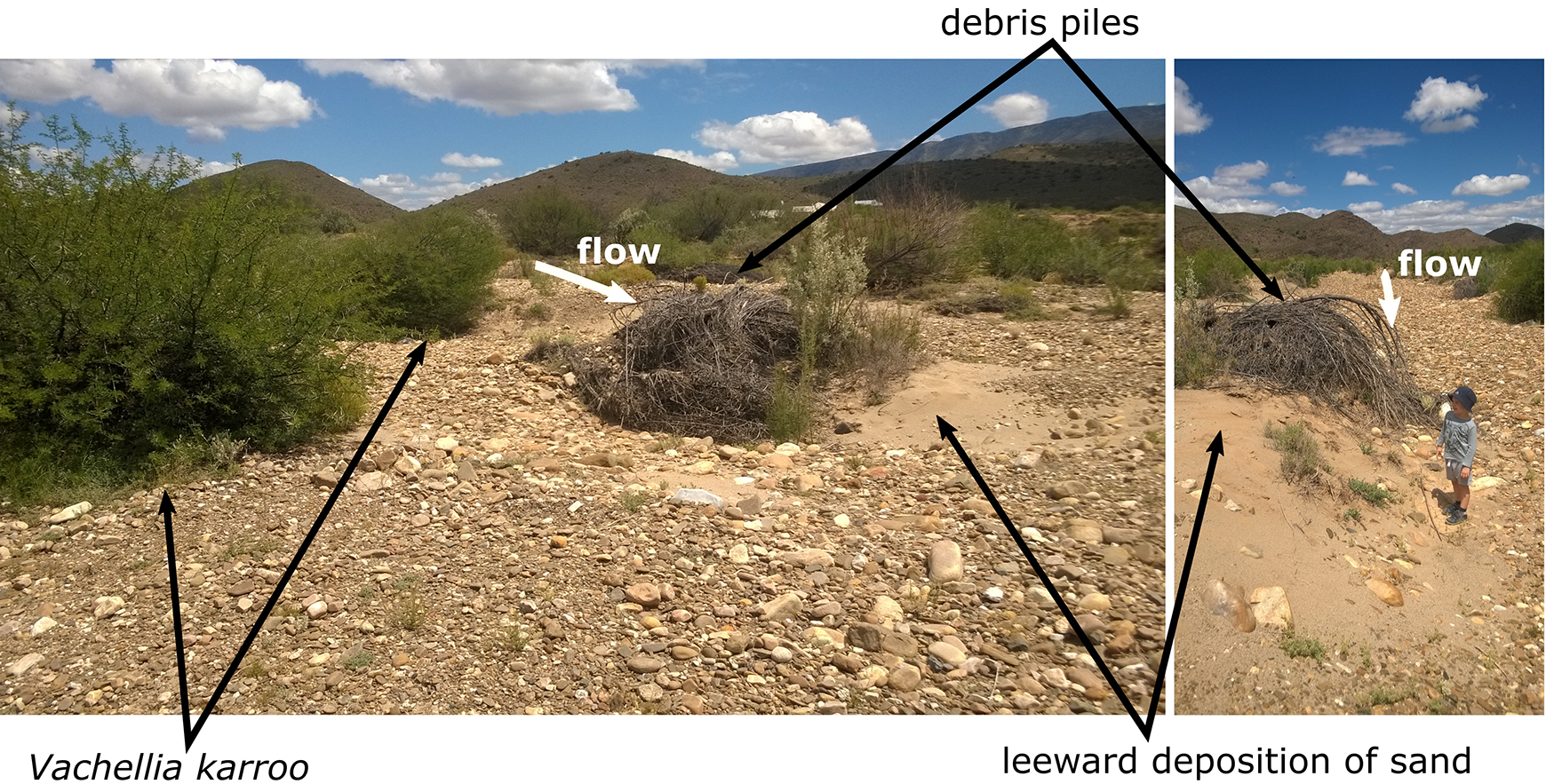
Photographs of forced debris-bar features and bed sediment patchiness that result from an interaction between Vachellia karroo woody-debris piles (in many cases, snagged against living thorn tree stems) and the transport of a mixed gravel-sand sediment load.

In light of the above, sediment transport was modelled using the approach of Van Rijn (1993), as this suite of transport relations explicitly captures the critical effects of local flow and sediment characteristics that facilitate the application of essentially steady-flow capacity formulations in ‘flashy’ flow environments (Cao et al., 2010). By tracking the transport of both the coarse gravel and the more readily suspendible medium sand, the Van Rijn (1993) approach is at least conceptually suited to a bed that partly comprises features composed of a mixture of clast sizes, and partly comprises patches dominated by one size or the other. Further research is needed to test these assertions, with modelling focused on a finer grid resolution than that presented in this paper. The sediment feed rate was calculated by the model, rather than imposed as an inlet boundary condition, by dynamically (in-sync with the flow time-series) replacing an equal proportion of sediment scoured at the inlet by the flow. Since field observations indicate that the system is neither characterised by net aggradation, nor net incision, comprising a mixture of channels, sediment bars, and small patches of exposed bedrock, the sediment feed approach described above is considered a reasonable point of departure (this is discussed further in Section IV).

Bed roughness was parameterised using a quadratic friction law, expressed in terms of a Chézy coefficient derived from the Manning equation using the formula:

C = \frac{H^{1/6}}{n}

where H is the water depth (m), and n is Manning’s roughness coefficient (estimated to be 0.045 following the exercise described in ‘The outlet stage discharge relation’ below, and considered to be a reasonable representation of domain-average roughness conditions). Application of a spatially uniform roughness parameterisation across a natural environment that displays spatial variation in particle size and vegetation patchiness is a concession required to predict morphological responses over decadal timescales for the purpose of this preliminary test of the approach. Only sub-grid scale roughness elements (e.g. related to the vegetation and sediment composition) are parameterised by the model, as the effects of larger features of channel irregularity that develop during the morphodynamic spin-up period and subsequent experimental variable flow inlet time-series are represented by the grid/morphology. The application of vegetation-based biomorphodynamic roughness parameterisations is discussed in Section IV (e.g. Bertoldi et al., 2014; Van Oorschot et al., 2016). Operationalisation of these parameterisations requires further research to establish realistic growth models for the dominant plant species (the native Vachellia karroo, and the emerging invasive Tamarix ramoisissima).

Turbulence was modelled using a zero-order eddy viscosity model (Uittenbogaard et al., 1992), with constant background coefficients of horizontal eddy viscosity (1) and eddy diffusivity (10). The direction of sediment transport was adjusted to account for the effects of secondary flow using a correction scheme in which the local streamline curvature provides the source term in a transport equation, which defines the equilibrium spiral flow intensity. Given that inset channels through the reach are relatively straight, while the valley floor is slightly sinuous, it is likely that strong secondary currents are only a feature of the hydraulics of flows that fill or exceed inset-channel capacity. The direction of sediment transport was also adjusted for the effects of gravity, which causes sediment to deviate from the near-bed flow direction slightly and move in the direction of the local bed slope (αbs was set to 10, and αbn was set to 15, following Banda et al., 2017).

2.3 The inlet flow time-series

There is some uncertainty in the accuracy with which the DWS discharge data represent inlet conditions at the proto-riverscape site, given that the gauging weir is located ∼18 km downstream of the site (along the valley axis), and is fed in this downstream reach by two tributaries draining the inland lee of the Langeberge, which is a relatively high rainfall part of the Touws catchment (Figure 3). Using observations of river flow (binary; ‘die Touw loop’ or ‘the Touw is flowing’) from 1977 to present, collected and curated by residents of Plathuis for the centre of the proto-riverscape reach (see Figure 3 for location) (cited hereafter as Reënval Plathuis), it was possible to filter the DWS flow record to exclude events recorded at the gauging station, but not at the reach of interest (Figure 6). Comparison of the DWS and Reënval Plathuis records revealed a total of 109 flow periods (flow observations/records separated by zero-flow values) between 1982 and 2017, with 32 flow periods common to both records, and 74 flow periods recorded at the DWS gauge, but not observed at Plathuis. The latter flow periods were excluded from the inlet flow time-series developed for the model as part of the filter exercise. Many of the largest floods on record appear to have been sourced more widely within the catchment, and had substantial contributions from the lower Brak and Prins tributary catchments (Figure 3), based on observations of the origin of flooding recorded in the Reënval Plathuis diary (Figure 6).

A total of three flows were noted in the Reënval Plathuis diary that evidently ceased/infiltrated before reaching the DWS gauge, while a further two such flows have been observed since the research programme commenced in 2017. These flows were sourced within the lower-middle catchment, and ended before the proto-riverscape site (2018 event) or before the downstream gauging weir (2019 event). Field observations indicate that these ‘local flows’ have had limited morphodynamic impact on the structure and configuration of geomorphic units, suggesting that they fall below the threshold for substantial entrainment of the bed material, but have been associated with surface flow connectivity and the ‘topping up’ of large pools, and with the deposition of a thin veneer of sand and finer material, all of which has biogeochemical and ecological implications (e.g. Boulton et al., 2017).

Figure 6.

DWS Okkerskraal (J1H018) gauged mean daily discharge record, with Reënval Plathuis Touws River and tributary flow observations indicated along the top of the graph.

Without any reasonable method to distinguish which flows observed at Plathuis were likely to be similar in magnitude to those recorded at the gauge, given the variability described, it was decided that the Reënval Plathuis-filtered DWS record would be used as the inlet flow time-series for the morphodynamic spin-up process, with the original DWS-recorded event magnitudes retained. The mean annual discharge of this filtered flow time-series is 0.73 m³/s, while the median is close to zero given a no-flow duration of ∼80% (the mean positive daily flow value is 2.68 m³/s, while the median positive daily flow value is 0.036 m³/s), with a range in flow from 0 to 1515 m³/s (Figure 6). Zero-flow periods were reduced to one day in duration for the modelling exercise for the sake of computational efficiency. This is sufficient for the domain to drain to the typical no-flow hydrological condition between flow periods or flood events. These zero-flow ‘spacers’ between flows were considered critical to the representation of natural morphodynamics, as most floods in the Touws River are rapid-rise events that arrive following a period of no flow and reach a peak within 24 to 48 hours, and differences in morphological outcomes were observed for inlet flow time-series simulations that did not include zero-flow spacers.

2.4 The outlet stage–discharge relation

A stage–discharge relation was developed for the outlet cross-section morphology using Manning’s Equation, with the incremental method of Chow (1959) applied to estimate Manning’s n, and constant water surface slope prescribed through the outlet. To fix this condition at the outlet, and faithfully represent the mixed bedrock-alluvial environment, the initial sediment thickness for the domain was specified using a file which set all cells in the domain to a uniform sediment thickness (1 m, following Nicholas et al., 2013; Sloff and Mosselman, 2012, and informed by field observations), except the line of cells across the outlet, where sediment thickness was set to zero. Fixing the outlet condition was a response to observations in early simulations of deep incision at the outlet, which propagated headward to influence the morphology of the partly confined area in particular, and which would be prevented in nature by the bedrock superimposition of the channel bed.

2.5 Summary of model development

The approach to inlet flow time-series development is similar in concept to the ‘representative hydrograph’ idea of Huthoff et al. (2010) and Sloff et al. (2006), but with more comprehensive representation of the variability observed over a ∼30-year period, rather than the typical seasonal variability represented in the cited works, given the aseasonal flow regime. The goal of the model development exercise was not to create an exact replica of the proto-riverscape environment in every minor detail, but to create a system that is similar to the natural prototype in critical ways, such that it exhibits similar characteristics, processes, and behaviour (e.g. Bras et al., 2003), and can be used to explore the effects of flow regime modification on the DRPV in quantifiable metrics of physical habitat suitability and diversity, and disturbance/renewal regimes. The simulations employed in this work had run-times of one to two weeks on a standalone workstation with a 3.3 GHz processor speed, but the machine could accommodate two to three simulations running concurrently.

3 Comparison of morphodynamic spin-up conditions with empirical observations

The end-point morphology of the morphodynamic spin-up run (driven by the Reënval Plathuis-filtered DWS flow record) represents the initial morphology for all subsequent flow modification experiment inlet flow time-series. This spin-up morphology was compared with empirical observations of the riverscape environment in profile and planform, to evaluate the extent to which the virtual riverscape represents the proto-riverscape. A map of planform dynamics for the proto-riverscape was prepared by digitising and overlaying inset channel locations from orthorectified and georeferenced digital aerial photography (Figure 7). The focus of this and other proto-riverscape-model comparisons is an area of interest (indicated in Figure 7) that lies beyond the influence of the inlet and outlet open domain boundaries. The spin-up period reorganises the initial (contour interpolated) morphology of the domain into a pattern of predominantly single-thread channel through partly confined parts of the riverscape (including the two most prominent pools, ‘a’ and ‘b’), and retains traces of a dual-thread pattern in laterally unconfined parts, especially within the widest upstream part of the domain (before pool ‘b’), where the macro-channel boundary is set back some distance from the inset channel. This is considered a reasonable approximation of channel pattern, noting that the empirical planform dynamics are displayed for a longer period than is represented by the flow time-series of the spin-up period.

Figure 7.

Post morphodynamic spin-up plan morphology in the context of ∼70 years of observed proto-riverscape planform dynamics. Flow is from left to right. A photograph of the pool denoted ‘b’ is shown in Figure 4. Large, persistent pools within the reach are located at points ‘a’ and ‘b’ as indicated.

The spin-up morphology was also compared with differential global positioning system (dGPS) field survey data available for a portion of the proto-riverscape (Figure 8). Changes in the orientation of the inset channel are less smooth than is indicated by the model spin-up morphology, and the relief at the inner bends of pools ‘a’ and ‘b’ appears to be more pronounced in nature than indicated. This may be a reason for the slight offset in the position of pool ‘b’ in the spin-up morphology relative to the proto-riverscape, where the pool is forced against a shale bedrock margin. It is encouraging, however, to note that the spin-up profile dimensions of the pools and the inset channel in general are in close agreement with those of the proto-riverscape, resulting in a virtual riverscape that is comparable to the natural system from the perspective of key elements of physical habitat (especially the pools, which serve as refugia to aquatic biota during no-flow periods; Section II). Greater realism may be achieved by using a smoothed version of a full domain field or aerial morphological survey as the initial pre-spin-up morphology, where resources allow. However, it must be emphasised that the purpose of the spin-up run is to evaluate how well the model produces an environment that displays similar morphodynamic behaviour to the proto-riverscape from an initial simplified condition. There would be less to learn by starting with a highly realistic representation of proto-riverscape morphology.

Figure 8.

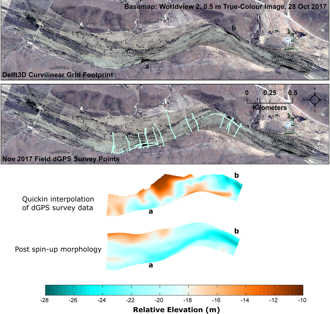
Post morphodynamic spin-up morphology in the context of dGPS surveyed field data, available only for the portion of the riverscape indicated. The dGPS data were interpolated to the model grid using Delft3D QUICKIN software triangular interpolation, with internal diffusion. Large, persistent pools within the reach are located at points ‘a’ and ‘b’ as indicated.

What is evident in the above comparison is the relative dominance of imposed (valley alignment) over flux (the inlet flow time-series) boundary conditions at this macro-scale of analysis. Several efforts to force pool ‘b’ to a more direct position of impingement against the bedrock margin (grid boundary) by using other inlet flow time-series (e.g. changing the sequence of events, running a constant maximum discharge, increasing the frequency of extreme events) and by increasing the grid resolution, had little effect. Imposed boundary conditions set the basic template of the domain, while the flux boundary conditions shape the finer details of features of physical habitat interest (Fryirs and Brierley, 2013). An exception to this may be the flux condition of vegetation growth dynamics, which can feed back to ‘fix’ features such as sediment bars in place for a sufficient duration to enforce topographic forcing of flow, although the sparse distribution of the dominant Vachellia karroo thorn trees in the proto-riverscape counts against this explanation (see Section IV.1, ‘Regional setting and study site description’). Persistent topographic forcing by the relief at the inner bend of pool ‘b’ may further be a consequence of induration of bar sediment common in environments with high atmospheric water demand, or a bedrock control obscured by overlying sediment.

4 Numerical experiment approach, and examples of model output

A simple comparison of two hypothetical future flow regime scenarios serves to illustrate how the effects of flow regime modification could be evaluated in an EWA exercise using morphodynamic modelling: i) a case where the historical flow regime is repeated in future (Figure 9; ‘historical flow regime experiment’); and ii) a case where low flows are largely eliminated (the no-flow duration is increased), intermediate flows are reduced, but large floods are retained (Figure 9; ‘modified flow regime experiment’). These are purely hypothetical scenarios, although the type of modification presented by case (ii) is a likely consequence of efforts to increase runoff harvesting within the catchment by damming and diverting ephemeral tributaries. An increase in this practice has been observed in the study area since the start of the research programme in 2017. The exact nature of the flow regime modification scenario would depend in practice on the type of water resource development under consideration (see, for example, the increase in flow pulse duration associated with flow releases from impoundments considered by Bunn et al., 2006), and management response scenarios could be better informed by the functional flows approach of Yarnell et al. (2020) in a full EWA exercise.

Figure 9.

DRPVm in the longitudinal flux connectivity of suspended sediment (sand and finer) and particulate resource base between the two main riverscape refugia (pools ‘a’ and ‘b’ in Figures 7 and 8) within the domain area of interest (lower graphs), in response to the experimental inlet flow time-series described in the text (upper graphs).

A wide array of spatially explicit hydrological/hydraulic (e.g. depth, depth-averaged velocity, Froude number) and sediment transport/composition data are recorded at each output time-step for a Delft3D simulation run. For the purpose of this initial demonstration of the approach, two examples of DRPVm in physical habitat are illustrated in Figures 9 and 10. The output time-step interval for experimental simulations was set to one day, to match the interval of the inlet flow time-series data. This ensures that a DRPVm can be developed from different types of model output that integrates the morphodynamic response of the virtual riverscape to inlet flow regime forcing. The first output example (Figure 9) illustrates a DRPVm in the longitudinal flux connectivity between the two main riverscape refugia within the domain area of interest (lower graphs), in response to the experiment inlet flow time-series described above (upper graphs). This is achieved by extracting from simulation output the total magnitude of depth-averaged suspended load transport (m³/s/m) for a cross-section between pools ‘a’ and ‘b’ for each output time-step. This information provides insight into sediment flux transfers between refugia, as well as fluxes of sediment-associated BREs that can influence pool physico-chemistry and resource availability to biota (Boulton et al., 2017; Burchsted et al., 2014; Jaeger et al., 2017; Von Schiller et al., 2017), and broader-scale biogeochemical cycling (Aufdenkampe et al., 2011). Comparison of the scenarios presented illustrates an overall reduction in flux connectivity for the modified flow regime, but also a more complex response in suspended load transport for the large flood near the end of each flow time-series scenario (between 4000 and 5000 hours for the historical flow regime, and between 3000 and 4000 hours for the modified flow regime); for the same flood peak magnitude at this point in the simulations, the modified flow regime scenario produces a larger suspended load flux. This may be due to local storage effects within the riverscape that are a result of reduced intermediate flows, and which result in a larger pulse in sediment flux through the system in association with the large flood. The cumulative total flux transfer for the modified flow regime scenario is ∼10% lower than that for the historical flow regime scenario. For non-perennial rivers, it is likely that this total flux difference would vary primarily as a function of modification of the large event record (Heritage et al., 1999; Jaeger et al., 2017; Rountree et al., 2001), which was not altered in the flow regime modification scenarios considered here.

The second example (Figure 10) illustrates a DRPVm in the surface-flow-inundation frequency for the full virtual riverscape environment. This is achieved by extracting from simulation output the magnitude of depth-averaged velocity for each cell for each output time-step, and then creating a composite image of the total number of positive velocity values in each cell as a percentage of the total flow time period, such that output frequencies of surface-flow-inundation activity are scaled for the true possible flow duration (the maximum inundation frequency of ∼20% in Figure 10 is consistent with the observed no-flow duration of ∼80% for the historical flow regime). Comparison of the scenarios shows an overall reduction in the spatio-temporal surface-flow-inundation activity for the modified flow regime scenario, as well as reduced surface flow connectivity within the laterally unconfined part of the riverscape (with implications for lateral flux dynamics; Boulton et al., 2017; Brierley and Fryirs, 2005; Thoms and Sheldon, 2002), and reduced surface flow activity in the key refugia (especially for pool ‘a’). Critically, this output takes account of morphodynamic development of the system over time, and is not simply a plot of hydro-dynamics on a static template.

Figure 10.

Riverscape spatio-temporal DRPVm in surface-flow-inundation frequency (and lateral flux connectivity for water and constituent resources), in response to the experimental inlet flow time-series described in the text (Figure 9; upper graphs). Large, persistent pools within the reach are located at points ‘a’ and ‘b’ as indicated.

Cumulative aerial extents may be further analysed using frequency histograms (Figure 10). For the modified flow regime scenario considered, there would be an overall increase in the aerial extent of no to low surface-flow-inundation frequency classes, and a decrease in the aerial extent of higher surface-flow-inundation frequency classes (and an effective loss of the highest frequency classes). Ongoing field investigations of surface and groundwater chemistry in the vicinity of pool ‘b’ that commenced in 2017 suggest that these changes would influence pool salinity dynamics in particular (e.g. Day et al., 2019; Gómez et al., 2017), in that sporadic surface flows are a primary source of relatively low salinity water to these systems. Under no flow conditions, pool ‘b’ is sustained by a low and highly variable rainfall and local runoff input, or a slow ‘bleed’ of highly saline groundwater discharge, such that a reduction in surface flow connectivity beyond the historical range of variability could lead to sustained dominance of salt-tolerant species, and reduced species turnover associated with freshening events (Day et al., 2019). A further study is underway to consider the potential implications for an emerging invasion of the alien Tamarix ramosissima, which is a salt-tolerant phreatophyte (CABI, 2019) and is, therefore, able to rapidly colonise saline pool margins, out-compete the native thorn trees, lead to enhanced drawdown of pool water levels by evapotranspiration (Cleverly et al., 2002), and potentially influence future morphodynamics (e.g. Rowntree, 1991). The same approach as that illustrated in Figure 10 may be applied to other physical habitat elements, such as the dominant substrate type (relative percentage of sand or gravel in the bed, in model output terms), or surface complexity, considered important for evaluating biotic responses in EWA (e.g. Scown et al., 2016).

Hydraulic indices such as the Froude number are among the standard set of spatially explicit model output, and could yield insight into the DRPVm in hydraulic biotope distributions in perennial rivers (Padmore, 1998; Wadeson and Rowntree, 1998). However, given the lengthy periods of hydraulic inactivity in non-perennial rivers, it is necessary to question the application of purely hydraulic indices of physical habitat developed for perennial rivers (both hydraulic biotope assessment, and eco-hydraulic models that impose a fluctuating water level on a static morphological template; Gore et al., 2001; James and King, 2010), as suggested by Petersen and Dollar (2007). It is at least necessary to clarify what duration of hydraulic activity is required for species of interest to initiate or complete their life cycles, and at what magnitude or duration of hydraulic activity does the diversity of hydraulic biotopes distributed across a river reach begin to influence species occurrence and distributions (e.g. Watson and Dallas, 2013). This is an area requiring further research (King and Schael, 2001; Seaman et al., 2010), with current evidence suggesting that a focus on macro-habitat indices would better serve EWA efforts in non-perennial rivers (De Farias et al., 2020; Thoms et al., 2006; Watson and Dallas, 2013).

V General implications for EWA, limitations, and future research needs

While some work has been done to conceptualise the impact of flow regime modification on sediment transport processes in dryland rivers (e.g. Heritage et al., 1997; Van Niekerk and Heritage, 1994), King et al. (2008) argued that the link between physical habitat, hydrology, and the distribution of biota could be better defined. In addition, they suggested that a major research priority for EWA is clarification of the importance of different magnitude flows in shaping physical habitat from reach to micro-habitat patch scales. The spatially integrated physical habitat diversity of a reach at a single point in time (e.g. the end-point of a simulation) is not a useful metric for EWA, especially where the ‘end point’ itself may be a transient physical state (e.g. Heritage et al., 1997; Rountree et al., 2001; Rowntree, 2013). Physical riverscape habitat results when water is overlaid upon (for surface water), or injected within (for groundwater) the sedi-morphological template. Thus, metrics of endpoint sedi-morphological diversity alone do not necessarily equate with biological diversity (Brierley and Fryirs, 2005), as this template retains some ‘memory’ of former flow regimes (an extreme example would be an environment of high sedi-morphological diversity from which water has been diverted, such that the environment has become essentially terrestrial in nature – morphological diversity that is ‘hydro-ecologically moot’). However, the integrated DRPVm in physical habitat expressed during the interaction of hydraulics, sediment transport, and morphological change (i.e. the morphodynamics) for a duration of system development can provide ecologists with new metrics of physical habitat that can enhance the management of non-perennial rivers.

The approach presented in this paper enhances the analysis of geomorphological effects of flow regime modification, and represents a point of departure toward addressing the limitations of present approaches to incorporating geomorphological information in EWA in South Africa, highlighted by King et al. (2008), Rowntree (2008), Rossouw et al. (2005) and Seaman et al. (2010, 2013, 2016). The approach begins to address present limitations by i) explicitly evaluating dynamic feedbacks between hydrology, sediment transport, and river morphology and substrate (which are presently considered only conceptually, or are not dynamically coupled); ii) considering a full range of hydrological variability to provide an understanding of the full range of morphodynamic variability (rather than the present approach of considering only a few flow levels); and iii) expanding the spatio-temporal reach of analysis beyond static cross-sections (the dominant practice at present) to dynamic riverscapes, where elements of physical habitat can be viewed by ecologists in four dimensions (Thoms and Sheldon, 2002; Ward, 1989).

The examples provided illustrate how metrics may be developed that provide insight into physical habitat suitability and diversity, and disturbance/renewal regimes (Thoms, 2006; Thoms et al., 2017), but also how morphodynamics might be linked with biogeochemistry (e.g. Gómez et al., 2017; Von Schiller et al., 2017) through consideration of flux dynamics and connectivity (Aufdenkampe et al., 2011; Boulton et al., 2017). These metrics (in both graphical form, as presented here, and in the form of simulation video output) may be applied by ecologists to develop species or ecosystem services response curves in decision-making frameworks such as DRIFT (King et al., 2003) or DRIFT-ARID (Seaman et al., 2013). However, care should be taken when interpreting these metrics to adopt an experimental mind-set; the results do not perfectly reflect ‘reality’ (as with any model), nor do they represent the future – they represent a possible future range of variability for the flow regime scenarios considered, and provide a tool to evaluate potential outcomes of flow regime modification from a physical habitat perspective. Further value of the approach lies in its capacity to explicitly evaluate a variety of outcomes for sensitivity-driven ranges of input variables that may be difficult to constrain through fieldwork alone (Kleinhans, 2010).

Although this initial work has been focused at the riverscape-reach scale, morphodynamic modelling can also be applied over larger spatial scales by reducing model dimensionality (e.g. 1D Delft3D), or by reducing the complexity of process representation (e.g. CAESAR-Lisflood; Milan et al., 2018a, 2018b). However, the physical habitat dynamics questions that may be addressed by approaches focused on different scales will likely differ (e.g. large-scale longitudinal flux connectivity rather than intra-reach linkages between refugia). Similarly, it may not always be necessary or desirable to explore a full riverscape response to flow regime modification, and much can be learned by focusing modelling efforts on smaller scales with particular features in mind – for example, i) determining necessary conditions for tree/debris-bar and local scour-pool formation from a flow/sediment regime perspective (Wohl et al., 2019), ii) developing a higher-resolution understanding of inter-refugia exchange-flux processes (Boulton et al., 2017), or iii) enhancing understanding of flow regime–vegetation–morphodynamics interactions for key species (Table 1).

Table 1.

Summary review of the incorporation of vegetation-related biomorphodynamic/ecomorphodynamic interactions in numerical morphodynamic modelling. Although there is limited representation of non-perennial rivers in this literature, many of the approaches developed cater to rivers with variable (sometimes highly variable) flow regimes.

River type and conceptual approach to understanding vegetation-related riverscape morphodynamic interactions	References
Conceptual; broadly applicable to braided rivers. Domain width of 300 m and longitudinal slope of 0.01.	Murray and Paola (2003)
Incorporation of vegetation effects in a cellular/rule-based model. Simple rule-based parameterisation of the effects of plant growth on sediment transport and bank strength, under constant dominant discharge conditions.	Murray and Paola (2003)
Conceptual; broadly applicable to rivers with largely stand-forming vegetation types.	Baptist et al. (2007)
Development of a vegetation physical trait-based Chézy roughness formulation.	Baptist et al. (2007)
Allier River, France (temperate gravel-bed river with a perennial but variable flow regime).	Crosato and Saleh (2011)
Application of Baptist et al. (2007) relations, incorporating vegetation effects within a two-dimensional (2D) morphodynamic model through simple rules for colonisation of bare sediment surfaces. Effects considered for both constant and variable inlet flow time-series.	Crosato and Saleh (2011)
Applicable to perennial gravel-bed rivers.	Li and Millar (2011)
Rule-based parameterisation of vegetation effects on shear stress within a 2D morphodynamic model, using a ‘friction angle’ calibration parameter. Constant inlet discharge.	Li and Millar (2011)
Focused on large sand-bed tropical/sub-tropical rivers, with perennial but variable flow regimes.	Nicholas (2013); Nicholas et al. (2013)
Rule-based representation of channel to floodplain conversion; active channel cells are converted to vegetated floodplain cells when the maximum depth of inundation experienced over a specified time period (Tveg) does not exceed a given threshold depth (Hcr).	Nicholas (2013); Nicholas et al. (2013)
Anabranching rivers in both Alpine and dryland settings. Considers both ‘stand-forming’ (continuous) and ‘obstacle-forming’ (spatially scattered) vegetation features.	Crouzy et al. (2016)
Physically based equations for simple continuous vegetation cover by grass to shrub-type vegetation, as well as a Kernel/neural-based approach to take account of the effects of vegetated obstacles. Explicit coupling with flow/sediment morphodynamics is a feature of the physically based model, while the Kernel model includes both long-range (non-local) and short-range vegetation interactions and feedbacks in a more simple way.	Crouzy et al. (2016)
Conceptual; linear stability analysis of effects of vegetation on channel planform and bed morphology.	Bärenbold et al. (2016)
Vegetation is modelled as a density field of rigid, emergent cylinders, affecting flow via a roughness change. Dynamic development and uprooting of vegetation are incorporated.	Bärenbold et al. (2016)
Medium-sized gravel-bed rivers such as the Magra River, Italy (Bertoldi et al., 2014), and Allier River, France (Kleinhans et al., 2018; Van Oorschot et al., 2016). Perennial but variable flow regimes.	Bertoldi et al. (2014); Van Oorschot et al. (2016); Kleinhans et al. (2018)
Dynamic representation of vegetation effects through integrated growth models coupled with a 2D morphodynamic model; effects on riverscape patterns and species populations.
Curueño River, a free-flowing gravel bed river in north-west Spain with a pluvio-nival hydrological regime (winter floods, summer low flows).	Martínez-Fernández et al. (2018)
Dynamic representation of vegetation effects through integrated growth models coupled with a 2D morphodynamic model; effects of climate change.	Martínez-Fernández et al. (2018)
Large channelised Alpine gravel-bed rivers presenting a pattern of variably vegetated alternate bars (e.g. Isère River). Variable flood regimes.	Jourdain et al. (2020)
Dynamic representation of vegetation effects through integrated growth models coupled with a 2D morphodynamic model; effects on the morphodynamics of alternate bars.	Jourdain et al. (2020)

Special attention has been paid in ecological applications of morphodynamic modelling (and elsewhere; e.g. Corenblit et al., 2015) to the dynamic effects of vegetation growth on physical riverscape patterns and processes (Figure 2; ‘biomorphodynamic filters’). While theoretical frameworks for the evaluation of vegetation effects on morphodynamics and physical habitat exist (see Camporeale et al., 2013, for an earlier review; Table 1), further work is needed in non-perennial rivers to develop appropriate species-level growth models for the dominant vegetation types (see Tooth, 2013, for examples), which must overcome greater variability in water availability, and generally greater evaporation-driven sediment salinity (Tooth and McCarthy, 2007). These natural stressors influence the nature of ‘windows of opportunity’ (sensu Kleinhans et al., 2018, 2019) for germination and establishment, thereby influencing the biomorphodynamic efficacy of riparian vegetation (Bertoldi et al., 2014). Non-perennial rivers display a diversity of vegetation patterns and densities (e.g. Dunkerley, 2014; Heritage et al., 1999; Li et al., 2015; Tooth and Nanson, 2004), and growth models must take account of both stand-forming and obstacle-forming vegetation features (e.g. Crouzy et al., 2016; Table 1), and the effects of debris (Wohl et al., 2019), given the prevalence of obstacle-scour pool interactions in rapid-rise non-perennial systems (Figure 5).

Further work is also needed to develop approaches to evaluating the environmental sediment requirements of non-perennial (and other) rivers (Edmonds, 2012; Pitlick and Wilcock, 2001; Wohl et al., 2015), especially for water resource developments such as dams that modify both flow and sediment regimes (Kondolf et al., 2014). Determining or predicting an inlet sediment concentration, and how this will be affected by a water resource development, is a major challenge to all approaches to incorporating geomorphological information in EWA (Seaman et al., 2010). Over relatively small spatial scales such as that represented in this paper, it can be assumed that most non-perennial systems will not be supply-limited for sediment for the morphodynamic spin-up/historical flow regime scenarios (Laronne and Reid, 1993). As the spatial scale increases, features such as in-channel wetlands or alluvial washes/floodouts (Jaeger et al., 2017) lead to longitudinal dis-connectivity (Brierley and Fryirs, 2005; Burchsted et al., 2014), and to transport-limitation, which is characteristic of dryland rivers at basin scale (Milliman and Farnsworth, 2011). There may be reaches located immediately downstream of features of dis-connectivity that are naturally locally supply-limited as a result. Episodic or sporadic slugs (sensu Nicholas et al., 1995) or waves of sediment entering a reach are also possible, but have been shown in ephemeral rivers to have a local, short-lived effect on the morphology, being readily reworked within a few years (Greenbaum and Bergman, 2006), due to the mobility of ephemeral riverbed sediment over a wide range of flows (Powell et al., 2001). With some consideration of riverscape dis-connectivity upstream of a reach of interest, therefore, it should be possible to arrive at a range of reasonable time-series approximations for the sediment feed, and to explicitly evaluate physical habitat sensitivity to this (in terms of DRPVm output, as illustrated in this paper).

The potential array of applications of morphodynamic modelling in EWA and other facets of fluvial ecosystems management is vast, and in a future of ever-increasing computing power, the feasibility of integrating field-informed morphodynamic modelling within existing management frameworks is certain to increase. There are already many cases where the additional time added by a modelling exercise is justified; in the context of current threats to global biodiversity from several sources of human impact (IPBES, 2019), it is imperative that we apply every available tool to evaluate impacts of anthropogenic activities, and to robustly inform fluvial ecosystems management, conservation, and restoration.

Footnotes

Acknowledgements

We thank the many landowners within the Touws River valley near Plathuis for their hospitality and interest in our research, especially those involved with the Touwsberg Private Nature Reserve, and Andre Hagen and Ashley Brownlee of Wolverfontein Karoo Cottages. The careful and conscientious citizen science effort of ‘Tannie Joan’, in collecting and curating local rainfall and river flow observations between 1979 and 2018, is acknowledged with thanks.

Declaration of conflicting interests

The authors have no conflicts of interest to declare.

Funding

The author(s) disclosed receipt of the following financial support for the research, authorship, and/or publication of this article: This work was funded by the University of the Western Cape Non-Perennial Rivers Research Programme.

ORCID iD

M.C. Grenfell

References

Acreman

Arthington

Colloff

, et al. (2014) Environmental flows for natural, hybrid, and novel riverine ecosystems in a changing world. Frontiers in Ecology and the Environment 12(8): 466–473.

Arboleda

Crosato

Middelkoop

(2010) Reconstructing the early 19th-century Waal River by means of a 2D physics-based numerical model. Hydrological processes 24(25): 3661–3675.

Aufdenkampe

Mayorga

Raymond

, et al. (2011) Riverine coupling of biogeochemical cycles between land, oceans, and atmosphere. Frontiers in Ecology and the Environment 9: 53–60.

Banda

Dittrich

Pervez

(2017) Morphodynamic modelling of a meandering sand bed river using Delft3D. In: Wieprecht

Haun

Weber

, et al. (eds) Proceedings of the 13th international symposium on river sedimentation, Stuttgart, Germany, 19-22 September 2016, pp. 551–558. London: Taylor & Francis.

Baptist

Babovic

Rodríguez Uthurburu

, et al. (2007) On inducing equations for vegetation resistance. Journal of Hydraulic Research 45(4): 435–450.

Bärenbold

Crouzy

Perona

(2016) Stability analysis of ecomorphodynamic equations. Water Resources Research 52(2): 1070–1088.

Bertoldi

Siviglia

Tettamanti

, et al. (2014) Modeling vegetation controls on fluvial morphological trajectories. Geophysical Research Letters 41: 7167–7175.

Biggs

Von Fumetti

Kelly-Quinn

(2017) The importance of small waterbodies for biodiversity and ecosystem services: Implications for policy makers. Hydrobiologia 793(1): 3–39.

Boulton

Rolls

Jaeger

, et al. (2017) Hydrological connectivity in intermittent rivers and ephemeral streams. In: Datry

Bonada

Boulton

(eds) Intermittent Rivers and Ephemeral Streams: Ecology and Management. 1st ed. London: Academic Press, Elsevier, 79–108.

10.

Bras

Tucker

Teles

(2003) Six myths about mathematical modeling in geomorphology. In: Wilcock

Iverson

(eds) Prediction in Geomorphology, Geophysical Monograph 135. Washington: American Geophysical Union, 63–79.

11.

Brierley

Fryirs

(2005) Geomorphology and River Management: Applications of the River Styles Framework. Oxford: Wiley-Blackwell.

12.

Brown

Pasternack

(2019) How to build a digital river. Earth-Science Reviews 194: 283–305.

13.

Brown

Pasternack

Lin

(2016) The topographic design of river channels for form-process linkages. Environmental Management 57(4): 929–942.

14.

Brown

Pasternack

Wallender

(2014) Synthetic river valleys: Creating prescribed topography for form-process inquiry and river rehabilitation design. Geomorphology 214: 40–55.

15.

Brunsden

Thornes

(1979) Landscape sensitivity and change. Transactions of the Institute of British Geographers 4(4): 463–484.

16.

Bunn

Thoms

Hamilton

, et al. (2006) Flow variability in dryland rivers: Boom, bust and the bits in between. River Research and Applications 22(2): 179–186.

17.

Burchsted

Daniels

Wohl

(2014) Introduction to the special issue on discontinuity of fluvial systems. Geomorphology 205: 1–4.

18.

CABI (Invasive Species Compendium) (2019) Tamarix ramosissima (salt cedar). Available at: https://www.cabi.org/isc/datasheet/52503 (accessed 1 May 2020).

19.

Camporeale

Perucca

Ridolfi

, et al. (2013) Modeling the interactions between river morphodynamics and riparian vegetation. Reviews of Geophysics 51(3): 379–414.

20.

Cao

Pender

(2010) Reconciled bedload sediment transport rates in ephemeral and perennial rivers. Earth Surface Processes and Landforms 35(14): 1655–1665.

21.

Chow

(1959) Open Channel Hydraulics. New York: McGraw-Hill.

22.

Cleverly

Dahm

Thibault

, et al. (2002) Seasonal estimates of actual evapo-transpiration from Tamarix ramosissima stands using three-dimensional eddy covariance. Journal of Arid Environments 52(2): 181–197.

23.

Corenblit

Davies

Steiger

, et al. (2015) Considering river structure and stability in the light of evolution: Feedbacks between riparian vegetation and hydrogeomorphology. Earth Surface Processes and Landforms 40(2): 189–207.

24.

Crosato

Saleh

(2011) Numerical study on the effects of floodplain vegetation on river planform style. Earth Surface Processes and Landforms 36(6): 711–720.

25.

Crouzy

Bärenbold

D’Odorico

, et al. (2016) Ecomorphodynamic approaches to river anabranching patterns. Advances in Water Resources 93: 156–165.

26.

Datry

Bonada

Boulton

(eds) (2017) Intermittent Rivers and Ephemeral Streams: Ecology and Management. 1st ed. London: Academic Press, Elsevier.

27.

Day

Malan

Malijani

, et al. (2019) Water quality in non-perennial rivers. Water SA 45(3): 487–500.

28.

De Almeida

GAM

Rodríguez

(2011) Understanding pool-riffle dynamics through continuous morphological simulations. Water Resources Research 47(1): W01502.

29.

De Almeida

GAM

Rodríguez

(2012) Spontaneous formation and degradation of pool-riffle morphology and sediment sorting using a simple fractional transport model. Geophysical Research Letters 39(6): L06407.

30.

De Farias

Stenert

Maltchik

, et al. (2020) Partitioning of macroinvertebrate assemblages across temporary pools in an intermittent dryland river. Inland Waters 10(4): 480–492.

31.

Delft3D Modelling

Guide

(2018) Delft3D modelling guidelines online resource. Available at: https://publicwiki.deltares.nl/display/D3DGUIDE/Delft3D+Modelling+Guide (accessed 1 May 2020).

32.

Dollar

ESJ

Rowntree

(2003) Geomorphological research for the conservation and management of Southern African Rivers (Vol. 2 Managing flow variability: The geomorphological response). Water Research Commission Report 849/2/03, Pretoria.

33.

Dollar

ESJ

James

Rogers

Thoms

(2007) A framework for interdisciplinary understanding of rivers as ecosystems. Geomorphology 89: 147–162.

34.

Dunkerley

(2014) Nature and hydro-geomorphic roles of trees and woody debris in a dryland ephemeral stream: Fowlers Creek, arid western New South Wales, Australia. Journal of Arid Environments 102: 40–49.

35.

Du Preez

Rowntree

(2006) Assessment of the Geomorphological Reference Condition. An Application for Resource Directed Measures and the River Health Programme. Water Research Commission Report 1306/1/06, Pretoria.

36.

Dyson

Bergkamp

Scanlon

(eds) (2003) Flow. The Essentials of Environmental Flows. 2nd ed. Gland and Cambridge: IUCN.

37.

Edmonds

(2012) Restoration sedimentology. Nature Geoscience 5(11): 758–759.

38.

Eze

Knight

(2018) A geomorphological characterisation of river systems in South Africa: A case study of the Sabie River. Physics and Chemistry of the Earth 105: 196–205.

39.

Ferguson

(1981) Channel form and channel changes. In: Lewin

(ed) British Rivers. London: Allen and Unwin, 90–125.

40.

Frissell

Bayles

(1996) Ecosystem management and the conservation of aquatic biodiversity and ecological integrity. Journal of the American Water Resources Association 32(2): 229–240.

41.

Frissell

Liss

Gresswell

, et al. (1997) A resource in crisis: Changing the measure of salmon management. In: Stouder

Bisson

Naiman

(eds) Pacific Salmon & their Ecosystems. Boston, MA: Springer, 411–444.

42.

Frissell

Liss

Warren

, et al. (1986) A hierarchical framework for stream habitat classification: Viewing streams in a watershed context. Environmental Management 10: 199–214.

43.

Fryirs

Brierley

(2013) Geomorphic Analysis of River Systems: An Approach to Reading the Landscape. Chichester: Wiley-Blackwell.

44.

Fryirs

Brierley

Erskine

(2012) Use of ergodic reasoning to reconstruct the historical range of variability and evolutionary trajectory of rivers. Earth Surface Processes and Landforms 37(7): 763–773.

45.

Gerritsen

de Goede

Platzek

, et al. (2008) Validation Document Delft3D-FLOW: A software system for 3D flow simulations. Deltares Technical Report Xo356, M3470, September.

46.

Gómez

Arce

Baldwin

, et al. (2017) Water physicochemistry in intermittent rivers and ephemeral streams. In: Datry

Bonada

Boulton

(eds) Intermittent Rivers and Ephemeral Streams: Ecology and Management. 1st ed. London: Academic Press, Elsevier, 109–134.

47.

Gore

Layzer

Mean

(2001) Macroinvertebrate instream flow studies after 20 years: A role in stream management and restoration. Regulated Rivers: Research and Management 17: 527–542.

48.

Greenbaum

Bergman

(2006) Formation and evacuation of a large gravel-bar deposited during a major flood in a Mediterranean ephemeral stream, Nahal Me’arot, NW Israel. Geomorphology 77(1–2): 169–186.

49.

Grenfell

Ellery

, et al. (2019) A genetic geomorphic classification system for southern African palustrine wetlands: Global implications for the management of wetlands in drylands. Frontiers in Environmental Science 7: 174.

50.

Grootboom

(2019) Investigating associations between fluvial style and the characteristics and distribution of geomorphic units in non-perennial rivers. Unpublished MSc Thesis, University of the Western Cape, South Africa. Available at: http://etd.uwc.ac.za/handle/11394/7149 (accessed 1 May 2020).

51.

Hamilton

Bunn

Thoms

, et al. (2005) Persistence of aquatic refugia between flow pulses in a dryland river system (Cooper Creek, Australia). Limnology and Oceanography 50(3): 743–754.

52.

Hattingh

(2020) Geomorphological controls on pool formation and pool persistence in non-perennial river systems. MSc Thesis, University of the Western Cape, South Africa.

53.

Heritage

Birkhead

Broadhurst

, et al. (1999) The influence of flooding on the erodibility of cohesive sediments along the Sabie River, South Africa. In: Smith

Rogers

(eds) Fluvial Sedimentology VI. Oxford: Blackwell, 131–145.

54.

Heritage

Entwistle

Milan

, et al. (2019) Quantifying and contextualising cyclone-driven, extreme flood magnitudes in bedrock-influenced dryland rivers. Advances in Water Research 123: 145–159.

55.

Heritage

Large

ARG

Moon

, et al. (2004) Channel hydraulics and geomorphic effects of an extreme flood event on the Sabie River, South Africa. Catena 58(2): 151–181.

56.

Heritage

Moon

Jewitt

, et al. (2001) The February 2000 floods on the Sabie River,South Africa: An examination of their magnitude and frequency. Koedoe 44(1): 37–44.

57.

Heritage

van Niekerk

Moon

, et al. (1997) The geomorphological response to changing flow regimes of the Sabie and Letaba river systems. Water Research Commission Report 376/1/97, Pretoria.

58.

Hillier

Sofia

Conway

(2015) Perspective – synthetic DEMs: A vital underpinning for the quantitative future of landform analysis? Earth Surface Dynamics 3(4): 587–598.

59.

Hooke

(2016) Morphological impacts of flow events of varying magnitude on ephemeral channels in a semiarid region. Geomorphology 252: 128–143.

60.

Huthoff

van Vuren

Barneveld

Scheel

(2010) On the importance of discharge variability in the morphodynamic modeling of rivers. In: Dittrich

Koll

Aberle

Geisenhainer

(eds) Conference Proceedings, River Flow 2010, 8-10 September 2010, pp. 985-992. Karlsruhe: Bundesanstalt für Wasserbau.

61.

IPBES (2019) Global assessment report on biodiversity and ecosystem services of the Intergovernmental Science-Policy Platform on Biodiversity and Ecosystem Services. Brondizio ES, Settele J, Ngo HT, and Díaz S (eds). IPBES secretariat, Bonn, Germany.

62.

Jaeger

Sutfin

Tooth

, et al. (2017) Geomorphology and sediment regimes of intermittent rivers and ephemeral streams. In: Datry

Bonada

Boulton

(eds) Intermittent Rivers and Ephemeral Streams: Ecology and Management. 1st ed. London: Academic Press, Elsevier, 21–49.

63.

James

King

(2010) Ecohydraulics for South African rivers: A review and guide. Water Research Commission Report 453/10, Pretoria.

64.

Jourdain

Claude

Tassi

, et al. (2020) Morphodynamics of alternate bars in the presence of riparian vegetation. Earth Surface Processes and Landforms 45(5): 1100–1122.

65.

King

Brown

(2006) Environmental flows: Striking the balance between development and resource protection. Ecology and Society 11(2): 26.

66.

King

Schael

(2001) Assessing the ecological relevance of a spatially-nested geomorphological hierarchy for river management. Water Research Commission Report 754/1/01, Pretoria.

67.

King

Brown

Sabet

(2003) A scenario-based holistic approach to environmental flow assessments for rivers. River Research and Applications 19: 619–639.

68.

King

Tharme

de Villiers

(eds) (2008) Environmental flow assessments for rivers: Manual for the Building Block Methodology (updated edition). Water Research Commission Report TT 354/08, Pretoria.

69.

Kleinhans

(2010) Sorting out river channel patterns. Progress in Physical Geography 34: 287–326.

70.

Kleinhans

de Vries

Braat

, et al. (2018) Living landscapes: Muddy and vegetated floodplain effects on fluvial pattern in an incised river. Earth Surface Processes and Landforms 43(14): 2948–2963.

71.

Kleinhans

Douma

Addink

(2019) Fate of pioneering vegetation patches in a dynamic meandering river. Earth Surface Processes and Landforms 44(8): 1618–1632.

72.

Knighton

Nanson

(1994) Waterholes and their significance in the anastomosing channel system of Cooper Creek, Australia. Geomorphology 9: 311–324.

73.

Knighton

Nanson

(1997) Distinctiveness, diversity and uniqueness in arid zone river systems. In: Thomas

DSG

(ed) Arid Zone Geomorphology: Process, Form and Change in Drylands. 2nd ed. Chichester: Wiley, 185–203.

74.

Knighton

Nanson

(2000) Waterholes form and process in the anastomosing channel system of Cooper Creek, Australia. Geomorphology 35: 101–117.

75.

Kondolf

Gao

Annandale

, et al. (2014) Sustainable sediment management in reservoirs and regulated rivers: Experiences from five continents. Earth’s Future 2: 256–280.

76.

Kotschy

Rogers

Carter

(2000) Patterns of change in reed cover and distribution in a seasonal riverine wetland in South Africa. Folia Geobotanica 35(4): 363–373.

77.

Landres

Morgan

Swanson

(1999) Overview of the use of natural variability concepts in managing ecological systems. Ecological Applications 9(4): 1179–1188.

78.

Laronne

Reid

(1993) Very high rates of bedload sediment transport by ephemeral desert rivers. Nature 366: 148–150.

79.

Laronne

Garcia

Reid

(2001) Mobility of patch sediment in gravel bed streams: Patch character and its implications for bedload. Gravel-Bed Rivers V, New Zealand Hydrological Society Inc., Wellington, New Zealand, 249–290.

80.

Laronne

Reid

Yitshak

, et al. (1994) The non-layering of gravel streambeds under ephemeral flood regimes. Journal of Hydrology 159(1–4): 353–363.

81.

Leigh

Boulton

Courtwright

, et al. (2016) Ecological research and management of intermittent rivers: An historical review and future directions. Freshwater Biology 61(8): 1181–1199.

82.

Leigh

Sheldon

Kingsford

, et al. (2010) Sequential floods drive ‘booms’ and wetland persistence in dryland rivers: A synthesis. Marine and Freshwater Research 61: 896–908.

83.

Lesser

Roelvink

van Kester

JATM

, et al. (2004) Development and validation of a three-dimensional morphological model. Journal of Coastal Engineering 51: 883–915.

84.

Bristow

Luthi

, et al. (2015) Dryland anabranching river morphodynamics: Río Capilla, Salar de Uyuni, Bolivia. Geomorphology 250: 282–297.

85.

Millar

(2011) A two-dimensional morphodynamic model of gravel-bed river with floodplain vegetation. Earth Surface Processes and Landforms 36(2): 190–202.

86.

Lynch

Schulze

(2007) Rainfall Database. In: Schulze

(ed) South African Atlas of Climatology and Agrohydrology. Water Research Commission Report 1489/1/06, Pretoria, Section 2.2.

87.

Makhonco

(2019) Hydrogeomorphic controls on the longitudinal distribution and dynamics of reed beds in non-perennial river systems, Western Cape, South Africa. MSc Thesis, University of the Western Cape, South Africa.

88.

Martínez-Fernández V, van Oorschot

de Smit

, et al. (2018) Modelling feedbacks between geomorphological and riparian vegetation responses under climate change in a Mediterranean context. Earth Surface Processes and Landforms 43(9): 1825–1835.

89.

Meitzen

Doyle

Thoms

, et al. (2013) Geomorphology within the interdisciplinary science of environmental flows. Geomorphology 200: 143–154.

90.

Milan

Heritage

Entwistle

, et al. (2018b) Morphodynamic simulation of sediment deposition patterns on a recently stripped bedrock anastomosed channel. Proceedings of the International Association of Hydrological Sciences 377: 51–56.

91.

Milan

Heritage

Tooth

, et al. (2018a) Morphodynamics of bedrock-influenced dryland rivers during extreme floods: Insights from the Kruger National Park, South Africa. Geological Society of America Bulletin 130: 1825–1841.

92.

Milan

Tooth

Heritage

(2020) Topographic, hydraulic, and vegetative controls on bar and island development in mixed bedrock-alluvial, multi-channeled, dryland rivers. Water Resources Research 56: WR026101.

93.

Milliman

Farnsworth

(2011) River Discharge to the Coastal Ocean: A Global Synthesis. Cambridge: Cambridge University Press.

94.

Mucina

Rutherford

(eds) (2006) The Vegetation of South Africa, Lesotho and Swaziland. Kirstenbosch, Cape Town: SANBI.

95.

Murray

Paola

(1994) A cellular model of braided rivers. Nature 371(6492): 54–57.

96.

Murray

Paola

(2003) Modelling the effect of vegetation on channel pattern in bedload rivers. Earth Surface Processes and Landforms 28: 131–143.

97.

NGI (2010) 5 m contour elevation dataset for South Africa. National Geospatial Information, Mowbray, Cape Town.

98.

Nicholas

(2013) Modelling the continuum of river channel patterns. Earth Surface Processes and Landforms 38(10): 1187–1196.

99.

Nicholas

Ashworth

Kirkby

, et al. (1995) Sediment slugs: Large-scale fluctuations in fluvial sediment transport rates and storage volumes. Progress in Physical Geography 19(4): 500–519.

100.

Nicholas

Ashworth

Sambrook Smith

, et al. (2013) Numerical simulation of bar and island morphodynamics in anabranching megarivers. Journal of Geophysical Research: Earth Surface 118(4): 2019–2044.

101.

Osterkamp

Hupp

(2010) Fluvial processes and vegetation – glimpses of the past, the present, and perhaps the future. Geomorphology 116(3–4): 274–285.

102.

Padmore

(1998) The role of physical biotopes in determining the conservation status and flow requirements of British rivers. Aquatic Ecosystem Health & Management 1(1): 25–35.

103.

Petersen

Dollar

ESJ

(2007) The geomorphology of dryland river ecosystems with special reference to their environmental flow requirements: a brief overview. Report prepared for the Faculty of Natural and Agricultural Sciences, University of the Free State, Environmental water requirements in non-perennial systems, Water Research Commission Contract No. 1587, Report No. CSIR/NRE/WR/ER/2007/0016/C. Stellenbosch: CSIR NRE.

104.

Petts

Amoros

(1996) The fluvial hydrosystem. In: Petts

Amoros

(eds.) The Fluvial Hydrosystems. Springer, Dordrecht. https://doi.org/10.1007/978-94-009-1491-9_1

105.

Pitlick

Wilcock

(2001) Relations between streamflow, sediment transport, and aquatic habitat in regulated rivers. In: Dorava

Montgomery

Palcsak

, et al. (eds) Geomorphic Processes and Riverine Habitat, Water Science and Application Vol. 4. Washington, DC: American Geophysical Union, 185–198.

106.

Poff

(2018) Beyond the natural flow regime? Broadening the hydro-ecological foundation to meet environmental flows challenges in a non-stationary world. Freshwater Biology 63: 1011–1021.

107.

Poff

Allan

Bain

, et al. (1997) The natural flow regime. BioScience 47(11): 769–784.

108.

Powell

Reid

Laronne

, et al. (1996) Bed load as a component of sediment yield from a semiarid watershed of the northern Negev. IAHS Publications-Series of Proceedings and Reports, International Association of Hydrological Sciences 236: 389–398.

109.

Powell

Reid

Laronne

(2001) Evolution of bed load grain size distribution with increasing flow strength and the effect of flow duration on the caliber of bed load sediment yield in ephemeral gravel bed rivers. Water Resources Research 37(5): 1463–1474.

110.

Puckridge

Sheldon

Walker

, et al. (1998) Flow variability and the ecology of large rivers. Marine and Freshwater Research 49(1): 55–72.

111.

Reid

Thoms

Chilcott

, et al. (2017) Sedimentation in dryland river waterholes: A threat to aquatic refugia? Marine and Freshwater Research 68(4): 668–685.

112.

Rhodes

McCullough

Espinosa

(1994) A coarse screening process for evaluation of the effects of land management activities on salmon spawning and rearing habitat in ESA consultations. Portland, OR: Columbia River Inter-Tribal Fish Commission.

113.

Rossouw

Avenant

Seaman

, et al. (2005) Environmental water requirements in non-perennial systems. Water Research Commission Report 1414/1/05, Pretoria.

114.

Rountree

Heritage

Rogers

(2001) In-channel metamorphosis in a semiarid, mixed bedrock/alluvial river system: Implications for instream flow requirements. IAHS 266: 113–123.

115.

Rountree

Rogers

Heritage

(2000) Landscape state change in the semi-arid Sabie River, Kruger National Park, in response to flood and drought. South African Geographical Journal 82(3): 173–181.

116.

Rowntree

(1991) An assessment of the potential impact of alien invasive vegetation on the geomorphology of river channels in South Africa. Southern African Journal of Aquatic Sciences 17(1–2): 28–43.

117.

Rowntree

(2013) Module B: Geomorphology Driver Assessment Index (River EcoClassification: Manual for EcoStatus Determination version 2). Department of Water Affairs and Forestry/Water Research Commission Report TT 551/13, Pretoria.

118.

Rowntree

(2008) Geomorphology. In: King

Tharme

de Villiers

(eds) Environmental Flow Assessments for Rivers: Manual for the Building Block Methodology. Updated edition. Water Research Commission Report TT 354/08, Pretoria, 169–194.

119.

Scown

Thoms

De Jager

(2016) An index of floodplain surface complexity. Hydrological Earth Systems Science 20: 431–441.

120.

Seaman

Avenant

Watson

, et al. (2010) Developing a method for determining the environmental water requirements for non-perennial systems. Water Research Commission Report TT 459/10, Pretoria.

121.

Seaman

Watson

Avenant

, et al. (2013) Testing a methodology for environmental water requirements in non-perennial rivers: The Mokolo River case study. Water Research Commission Report TT 579/13, Pretoria.

122.

Seaman

Watson

Avenant

, et al. (2016) DRIFT-ARID: Application of a method for environmental water requirements (EWR’s) in a non-perennial river (Mokolo River) in South Africa. Water SA 42(3): 368–383.

123.

Schulze

Maharaj

(2007) A-pan equivalent reference potential evaporation. In: Schulze

(ed) South African Atlas of Climatology and Agrohydrology. Water Research Commission Report 1489/1/06 Section 13.2, Pretoria.

124.

Sheldon

Bunn

Hughes

, et al. (2010) Ecological roles and threats to aquatic refugia in arid landscapes: Dryland river waterholes. Marine and Freshwater Research 61: 885–895.

125.

Singh

Crosato

Giri

, et al. (2017) Sediment heterogeneity and mobility in the morphodynamic modelling of gravel-bed braided rivers. Advances in Water Resources 104: 127–144.

126.

Sloff

Ottevanger

van Schijndel

SAH

(2006) Improvement of navigation channel Vianen (in Dutch). Report Q4200, WL|Delft Hydraulics, Delft, the Netherlands.

127.

Sloff

Mosselman

(2012) Bifurcation modelling in a meandering gravel-sand bed river. Earth Surface Processes and Landforms 37: 1556–1566.

128.

TANAP (2019) Introduction to the resolutions of the Council of Policy of Cape of Good Hope. Available at: http://www.tanap.net/content/activities/documents/resolutions_Cape_of_Good_Hope/introduction_english/38.htm (accessed 1 May 2020).

129.

Tharme

(2003) A global perspective on environmental flow assessment: Emerging trends in the development and application of environmental flow methodologies for rivers. River Research and Applications 19(5–6): 397–441.

130.

Thoms

(2006) Variability in riverine ecosystems. River Research and Applications 22: 115–121.

131.

Thoms

Sheldon

(2002) An ecosystem approach for determining environmental water allocations in Australian dryland river systems: the role of geomorphology. Geomorphology 47: 153–168.

132.

Thoms

Delong

(2018) Ecosystem responses to water resource developments in a large dryland river. Water Resources Research 54(9): 6643–6655.

133.

Thoms

Parsons

(2002) Eco-geomorphology: An interdisciplinary approach to river science. IAHS 276: 113–119.

134.

Thoms

Sheldon

(2000) Water resource development and hydrological change in a large dryland river: The Barwon-Darling River, Australia. Journal of Hydrology 228: 10–21.

135.

Thoms

Beyer

Rogers

(2006) Variability, complexity and diversity – The geomorphology of river ecosystems in dryland regions. In: Kingsford

(ed) The Ecology of Desert Rivers. Cambridge, UK: Cambridge University Press, 47–75.

136.

Thoms

Delong

Flotemersch

, et al. (2017) Physical heterogeneity and aquatic community function in river networks: A case study from the Kanawha River Basin, USA. Geomorphology 290: 277–287.

137.

Thorp

Thoms

Delong

(2006) The riverine ecosystem synthesis: Biocomplexity in river networks across space and time. River Research and Applications 22(2): 123–147.

138.

Tooth

(2012) Arid geomorphology: Changing perspectives on timescales of change. Progress in Physical Geography 36(2): 262–284.

139.

Tooth

(2013) Dryland fluvial environments: Assessing distinctiveness and diversity from a global perspective. In: Shroder

Wohl

(eds) Treatise on Geomorphology. San Diego: Academic Press, 612–644.

140.

Tooth

McCarthy

(2007) Wetlands in drylands: Geomorphological and sedimentological characteristics, with emphasis on examples from southern Africa. Progress in Physical Geography 31(1): 3–41.

141.

Tooth

Nanson

(2004) Forms and processes of two highly contrasting rivers in arid central Australia, and the implications for channel-pattern discrimination and prediction. Geological Society of America Bulletin 116: 802–816.

142.

Uittenbogaard

van Kester

JATM

Stelling

(1992) Implementation of three turbulence models in 3D-TRISULA for rectangular grids. Technical Report Z81, WL/Delft Hydraulics, Delft, the Netherlands.

143.

UNEP (1997) World Atlas of Desertification. 2nd ed. London: Edward Arnold.

144.

Uys

O’Keeffe

(1997) Simple words and fuzzy zones: Early directions for temporary river research in South Africa. Environmental Management 21: 517–531.

145.

Van der Wegen

Dastgheib

Jaffe

, et al. (2011) Bed composition generation for morphodynamic modeling: Case study of San Pablo Bay in California, USA. Ocean Dynamics 61(2–3): 173–186.

146.

Van Niekerk

Heritage

(1994) Geomorphology of the Sabie River: Overview and classification. Centre for Water in the Environment Report No. 2/93. Centre for Water in the Environment, University of the Witwatersrand, Johannesburg.

147.

Van Oorschot

Kleinhans

Geerling

, et al. (2016) Distinct patterns of interaction between vegetation and morphodynamics. Earth Surface Processes and Landforms 41(6): 791–808.

148.

Van Rijn

(1993) Principles of Sediment Transport in Rivers, Estuaries and Coastal Seas. Blokzijl, The Netherlands: Aqua Publications.

149.

Vannote

Minshall

Cummins

Sedell

Cushing

(1980) The River Continuum Concept. Canadian Journal of Fisheries and Aquatic Sciences 37: 130–137.

150.

Von Schiller

Bernal

Dahm

, et al. (2017) Nutrient and organic matter dynamics in intermittent rivers and ephemeral streams. In: Datry

Bonada

Boulton

(eds) Intermittent Rivers and Ephemeral Streams: Ecology and Management. 1st ed. London: Academic Press, Elsevier, 135–160.

151.

Wadeson

Rowntree

(1998) Application of the hydraulic biotope concept to the classification of instream habitats. Aquatic Ecosystem Health & Management 1(2): 143–157.

152.

Ward

(1989) The four-dimensional nature of lotic ecosystems. Journal of the North American Benthological Society 8(1): 2–8.

153.

Ward

Malard

Tockner

(2002) Landscape ecology: A framework for integrating pattern and process in river corridors. Landscape Ecology 17(1): 35–45.

154.

Ward

Tockner

Schiemer

(1999) Biodiversity of floodplain river ecosystems: Ecotones and connectivity. River Research and Applications 15(1–3): 125–139.

155.

Ward

Tockner

Uehlinger

, et al. (2001) Understanding natural patterns and processes in river corridors as the basis for effective river restoration. Regulated Rivers: Research & Management 17(4–5): 311–323.

156.

Watson

Dallas

(2013) Bioassessment in ephemeral rivers: Constraints and challenges in applying macroinvertebrate sampling protocols. African Journal of Aquatic Science 38(1): 35–51.

157.

Wohl

Bledsoe

Jacobson

, et al. (2015) The natural sediment regime in rivers: Broadening the foundation for ecosystem management. BioScience 65(4): 358–371.

158.

Wohl

Kramer

Ruiz-Villanueva

, et al. (2019) The natural wood regime in rivers. BioScience 69(4): 259–273.

159.

Yarnell

Stein

Webb

, et al. (2020) A functional flows approach to selecting ecologically relevant flow metrics for environmental flow applications. River Research and Applications 36(2): 318–324.