Ensemble learning based on remote sensing data for monitoring agricultural drought in major winter wheat-producing areas of China

Abstract

Drought is mainly triggered by the lack of precipitation, which can lead to insufficient water supply for crops thus affecting their growth and development. Reliable drought monitoring is crucial to understanding drought risk and avoiding drought-induced crop yield losses. Based on the Stacking regression method and multiple remotely-sensed drought factors from 2001 to 2017, this study developed an ensemble learning framework for monitoring agricultural drought in major winter wheat-producing areas in China. Stacking used five machine learning algorithms, namely, extreme gradient boosting, support vector regression, extra trees, and multi-layer perceptron, as the base learners to model the relationship between remote sensing drought factors and 1-, 3-, and 6-month standardized precipitation evapotranspiration index (SPEI). In this study, county-level winter wheat yield records and drought maps provided by the Global SPEI database (SPEIbase) were adopted to assess the suitability of Stacking-predicted SPEI drought maps in agricultural drought monitoring. The results show that Stacking outperformed other machine learning algorithms in terms of estimation accuracy, with the highest R² value of 0.77 and the lowest root mean square error (RMSE) of 0.47. The longer the time scale of model-predicted SPEI, the higher its correlation with detrended winter wheat yields. The comparison with the drought maps of SPEIbase shows that the Stacking-predicted drought maps successfully captured the spatial pattern and intensity change of drought events. The approach presented in the study has good applicability for agricultural drought monitoring and could be extended to the rest of the areas.

Keywords

agricultural drought standardized precipitation evapotranspiration index ensemble learning remote sensing drought monitoring

I Introduction

Drought, recognized as a highly destructive and frequent natural calamity, caused incalculable losses to water resources and agricultural productivity (Jiang et al., 2015; Yu et al., 2019). The characteristics of wide coverage and repeated occurrence make drought have widespread negative effects on agriculture, ecology, economy, and other fields (Du et al., 2013; Potopová et al., 2015). Drought usually begins with persistent precipitation deficiency and can be roughly differentiated into four categories according to its influencing mechanism, that is, meteorological drought, agricultural drought, hydrological drought, and socio-economic drought (Nicholls and Neville, 1997; Wilhite and Glantz, 1985).

The four types of drought are interrelated, where agricultural drought is usually triggered by the loss of available soil moisture due to meteorological drought, which leads to lower crop yields and threatens regional food security (Lu et al., 2020; Zhang et al., 2017). Overall, the severity and spatial pattern of agricultural drought vary significantly with region and time. Hence, there are challenges in determining the moment of the occurrence and termination of agricultural drought and in quantifying the dynamics of its scope and intensity (Touma et al., 2015; Wilhite, 2000). China has had numerous droughts recently, which pose serious challenges to crop output and food security (Hu et al., 2010; Wang et al., 2016). Therefore, precise and almost real-time drought monitoring is extremely important practically for ensuring regional food security. Specifically, advanced drought prediction systems can provide farmers and government decision-makers with critical drought information, helping them take timely measures to reduce the risk of crop output losses brought on by drought.

Reflecting the intensity and duration of drought events through suitable drought indices is a common practice to assess and monitor agricultural drought. Many indices have been created and widely used to identify the traits of drought events. Representative indices are Palmer Drought Severity Index (PDSI) (Palmer, 1965), Standardized Precipitation Index (SPI) (McKee et al., 1993), and Standardized Precipitation Evapotranspiration Index (SPEI) (Vicente-Serrano et al., 2010a). Both SPI and SPEI have multi-scalar characteristics that enable them to distinguish drought events at a more flexible time scale than PDSI. Unlike SPI, SPEI considers the effect of temperature and incorporates evapotranspiration into its calculation equation. Various drought indices were used to assess the influence of drought on crop yields to test their applicability in monitoring agricultural drought. Vicente-Serrano et al. (2012) assessed different drought indices on a global scale using several hydrological, agricultural and ecological reference data. Standardized precipitation evapotranspiration index was found to provide more useful information on agricultural drought than SPI and PDSI, and its associations with soil moisture and crop yields were stronger in most regions of the world than the other two indices. Tian et al. (2018) evaluated the effectiveness of six drought indices in monitoring agricultural drought in the south-central U.S. using soil moisture and yields from three crop fields. The results show that SPEI was more effective than other indices in reflecting soil moisture conditions and also highly correlated with crop yields. Therefore, SPEI has good performance in identifying the impact of drought on agriculture, and deserves to be widely utilized to track agricultural drought.

Traditional drought monitoring methods mainly rely on the drought indices like PDSI, SPI, and SPEI that were created using station-recorded data. Although station-based drought indices can accurately describe the drought events occurring around stations, they are not suitable for assessing the spatial patterns of drought on a regional scale (Park et al., 2016). Through the spatial interpolation method, station-based measurements can be used to estimate drought conditions in regions without station-based records, but this introduces considerable uncertainty to drought monitoring, especially in regions with a scarce or uneven distribution of stations (Swain et al., 2011). Remote sensing technology, with its wide coverage and timely observation, can improve regional drought monitoring by providing data that are continuous in time and space (Quiring and Ganesh, 2010; Sun et al., 2017). Numerous drought-related indices had developed through satellite remote sensing products to characterize the spatial aspects of drought, e.x., Normalized Difference Vegetation Index (NDVI) (Rouse et al., 1974), Normalized Difference Drought Index (NDDI) (Gu et al., 2007), Normalized Difference Water Index (NDWI) (Gao, 1996), and Normalized Multi-band Drought Index (NMDI) (Wang and Qu, 2007). However, affected by atmospheric conditions and inversion algorithms, the quality problems of remote sensing data may affect the quantification of drought by remote sensing drought indices, making the estimation accuracy of these indices inferior to that of station-based drought indices (Zhang and Jia, 2013). Therefore, fusing remote sensing data from multiple sources to simulate station-based drought indices may be an effective method to increase the precision of large-scale drought monitoring.

Researchers have attempted to assess regional drought conditions by establishing response relationships between multi-source data and station-based drought indices through different data-driven models. Given the complex effects of multiple environmental factors on drought, traditional regression models and probability models have limitations in dealing with the nonlinear relationship between variables in drought prediction (Chen et al., 2012; Li et al., 2016). In contrast, advanced machine learning methods relying on their powerful ability in extracting nonlinear relationships between drought factors and reference indices were considered suitable for integrating multi-source data to reproduce station-based drought indices (Feng et al., 2019; Mokhtar et al., 2021). Feng et al. (2019) estimated station-based SPEI using three machine learning models and 30 remote sensing drought indicators in southeastern Australia. The model reproduced the reference SPEI well (the maximum R² was about 0.9), and the generated drought maps were highly consistent with that of ground stations. Park et al. (2016) selected three artificial intelligence models that integrated 16 drought factors to predict station-based SPI. The model explained up to 95% of the SPI variability in the southern United States, with a strong agreement between predicted drought maps and U.S. Drought Monitor (USDM) maps.

We focus on developing an ensemble learning model using multiple remotely-sensed drought factors from 2001 to 2017. Station-based SPEI and county-level winter wheat yields were utilized as reference variables to explore the applicability of the ensemble in monitoring agricultural drought in the main winter wheat-producing areas of China. This study’s main goals were (1) to assess the accuracy of different models for simulating SPEI in relatively dry and relatively humid regions, respectively; (2) to quantify the relative importance of variables in predicting SPEI through machine learning models; (3) to explore the correlation between model-predicted drought maps and yield records, and evaluate the performance of yield prediction using SPEI maps, and (4) to compare the consistency between model-predicted drought maps and those provided by the Global SPEI database (SPEIbase).

II Materials

2.1 Study area

The study location (110°E-122°E, 29°N-40°N) is situated in the primary winter wheat-growing area of eastern China (Figure 1). It comprises 444 primary winter wheat-producing counties across a total area of nearly 5.5×10⁵ km². Winter wheat planting area accounts for about 75% of China’s (http://www.stats.gov.cn/, 2015). The study area is divided into north and south parts by the Huaihe River, with a warm temperate monsoon climate in the north and subtropical monsoon climate in the south. The annual precipitation and average annual temperature range from 500 to 900 mm and from 14 to 15°C, respectively, and both show a spatial distribution that decreased with increasing latitude from south to north. There are obvious regional and interannual differences in precipitation, and it is concentrated in summer. Compared with the rest of China, drought events occurred most frequently in the study area, which posed a serious risk to China’s winter wheat yields (Fu and Gang, 2002; Liu et al., 2015).

Figure 1.

Locations of the research area, weather stations, and winter wheat planting area.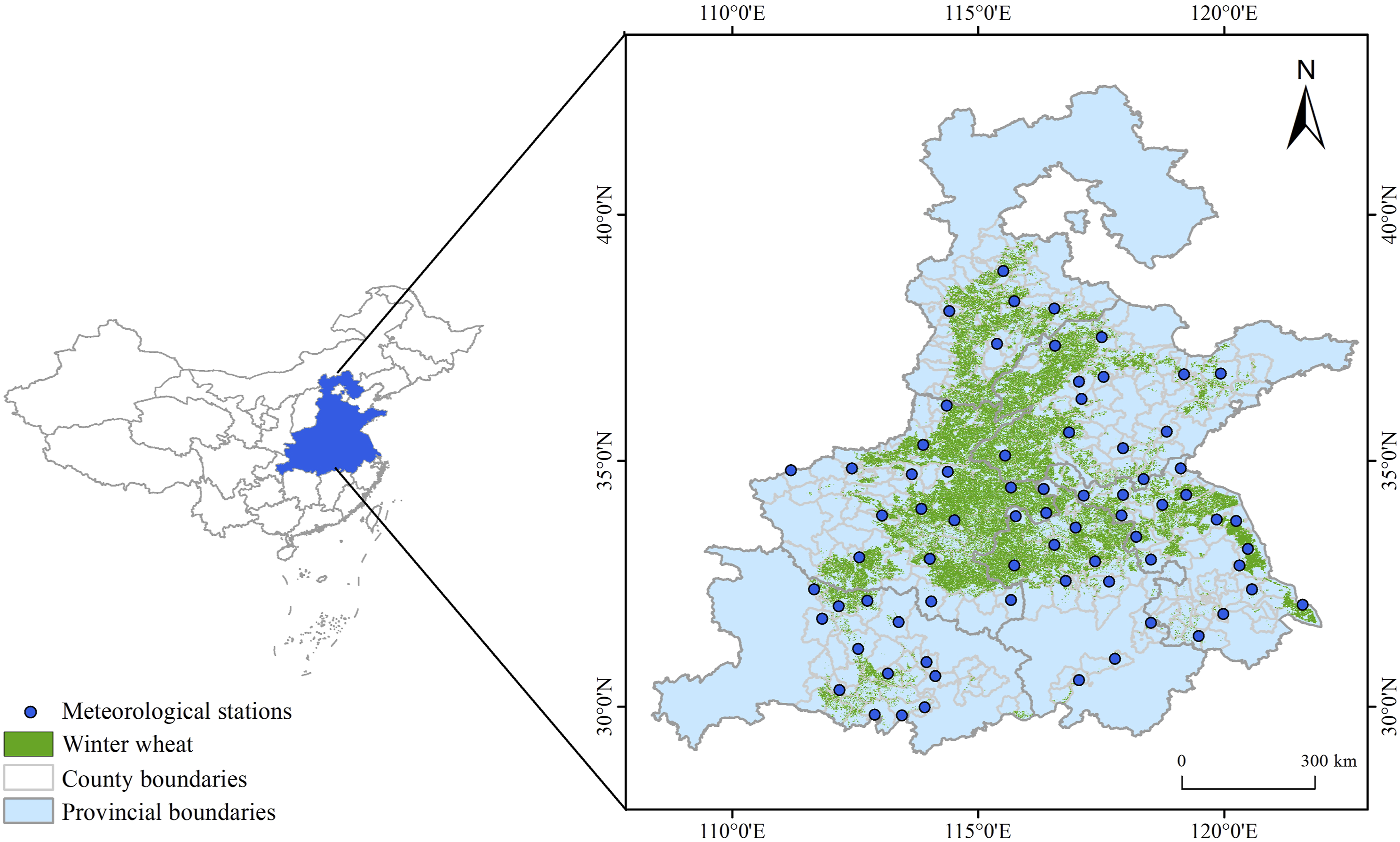

2.2 Data and preprocessing

2.2.1 Winter wheat cropping areas

To accurately reflect the drought situation of winter wheat in the research area, we adopted the annual winter wheat planting map at 1 km resolution provided by Luo et al. (2020) to mask the non-winter wheat cropping regions. In particular, the winter wheat cropping maps from 2001 to 2017 were synthesized into one image, in which the pixels that had been winter wheat farmland for more than 10 years were identified as winter wheat planting pixels. Subsequent yield-related calculations and visualizations were based on winter wheat planting pixels.

2.2.2 Remote sensing data

Drought indices for 2001–2017 were collected from various products of MODIS (Moderate Resolution Imaging Spectroradiometer) (Table 1). We acquired 8-day surface reflectance data with 500 m resolution from the MOD09A1 product and calculated NDWI, NDDI, and NMDI using the bands of surface reflectance. In particular, three alternative NDWIs were determined using bands 5, 6, and 7 respectively, and then were applied to the calculation of three different NDDIs (i.e., NDDI5, NDDI6, and NDDI7). NDVI data from the MOD13A2 product with 1 km and 16-day resolution. Eight-day Land Surface Temperature (LST) data at 500 m resolution were derived from the MOD11A2 product, and the mean (LSTm) of day LST (LSTd) and night LST (LSTn) was calculated. Evapotranspiration (ET) and Potential Evapotranspiration (PET) (at 500 m and 8-day resolution) were extracted from the MOD16A2 product. Additionally, we acquired monthly precipitation (Pre, 0.25°) from the Tropical Rainfall Measuring Mission (TRMM) product (3B43).

Table 1.

Summary of remote sensing-based drought indexes and their calculation formulas.

Drought indices	Formula
Pre	—
ET	—
PET	—
LSTd	—
LSTn	—
LSTm	(LSTd + LSTn)/2
NDVI	—
NDWI5, 6 & 7	(b2 - b5 (or 6 or 7))/(b2 + b5 (or 6 or 7))
NDDI5, 6 & 7	(NDVI - NDWI5 (or 6 or 7))/(NDVI + NDWI5 (or 6 or 7))
NMDI	(b2 - (b6 - b7))/(b2 + (b6 - b7))

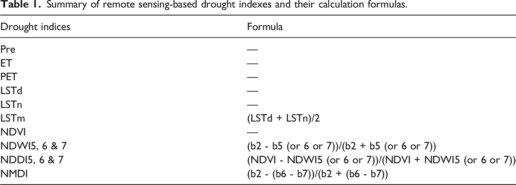
To account for the lagged response of agricultural drought to climate change, the 1-, 3-, and 6-month time scale averages of all climate variables (i.e., Pre, ET, PET, LSTd, LSTn, and LSTm) were calculated and used as inputs. In addition, the resolution of all variable data was unified to 1 km to match that of the winter wheat cropping map. The acquisition and processing of the above 26 variables were accomplished on the Google Earth Engine (GEE) platform. It is worth noting that crop growth responses to climate change vary by region, and the same prediction model was applied to data from various regions. Therefore, the anomaly of the variables during 2001–2017 was calculated using the following formula for each pixel.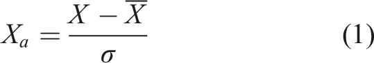

X_{a} = \frac{X - \bar{X}}{σ}

(1)

where

X_{a}

represents the anomaly of the variable in a certain month; X represents the variable in a certain month;

\bar{X}

is the average of the variable from 2001 to 2017; and σ is the standard deviation of the variable from 2001 to 2017.

2.2.3 Meteorological station data

Daily-scale ground observation data of 72 weather stations offered by the China Meteorological Administration (http://data.cma.cn/) were used. We chose SPEI as the reference data for monitoring meteorological drought, which reflects drought by normalizing the difference between precipitation and PET. Standardized precipitation evapotranspiration index values less than −1 are usually defined as drought conditions. In general, SPEIs on the time scale of 1 to 6-month are appropriate for monitoring agricultural drought. Therefore, according to the monthly precipitation and temperature data aggregated by the station data, the SPEIs on the time scale of 1-, 3-, and 6-month were calculated respectively, and PET was calculated by the “Thornthwaite” method (Thornthwaite, 1948). All the computations were realized by the “Climate Indices” package coded in the Python language.

2.2.4 Crop yield and irrigation rate data

In this study, winter wheat yield records were utilized to validate the potential suitability of drought predicted by the model. It is generally believed that under the condition of lower irrigation density, crop yields may be more correlated with drought conditions. Therefore, to more precisely assess the monitoring results of agricultural drought, we obtained gridded irrigation rate data from the Food and Agriculture Organization of the United Nations (FAO, https://www.fao.org/). By calculating the average irrigation rate of winter wheat planting pixels in each county in the study region, we selected the winter wheat yield of counties with an irrigation rate of less than 15% as the reference data for monitoring agricultural drought. The Statistical Yearbook provided data on winter wheat yields at the county level for the years 2001 to 2015. The typical planting and harvest dates for winter wheat in the research area are October and June.

It is worth noting that numerous factors affect crop yields, and our goal is to explore the impact of drought on crop growth, so the nonlinear growth trend of yields caused by variety improvement and agricultural technology development should be eliminated. The first-difference method proposed by Nicholls and Neville (1997) was used to separate the yield difference due to climate change from the growth trend.

III Methods

3.1 Modeling process

The process of assessing agricultural drought using drought factors based on remote sensing data in this study was summarized in Figure 2. There are two phases to the whole framework, the initial phase, firstly, the average of all variables’ anomaly within a 3 km × 3 km area around each station was extracted to predict the SPEIs at three time scales. Considering that the prediction ability of drought factors to SPEIs may be different in arid or humid areas, we used the K-means model (Hartigan and Wong, 1979) to divide meteorological stations into two clusters based on the average annual precipitation observed by the stations during 2001 to 2017. The mean annual precipitation and temperature for the two clusters were shown in Table S1, and as compared to stations in cluster 2, those in cluster 1 are comparatively drier. Next, we adopted four common machine learning algorithms (i.e., extreme gradient boosting (XGB), support vector regression (SVR), ET, and MLP) and an ensemble learning model (i.e., Stacking), which were integrated with remotely-sensed drought factors to estimate SPEIs indicators. For two clusters of stations, the models with the highest prediction accuracy were determined respectively. In the second phase, the average annual precipitation data from 2001 to 2017 calculated by remotely-sensed monthly precipitation data was applied to the K-means clustering model, and the cropping pixels in the research regions were split into two clusters. SPEI map was then generated by the optimal model corresponding to each cluster, and its effectiveness was tested by analyzing the consistency of the observed SPEI and SPEIbase datasets.

Figure 2.

Schematic flowchart of processes used in the study.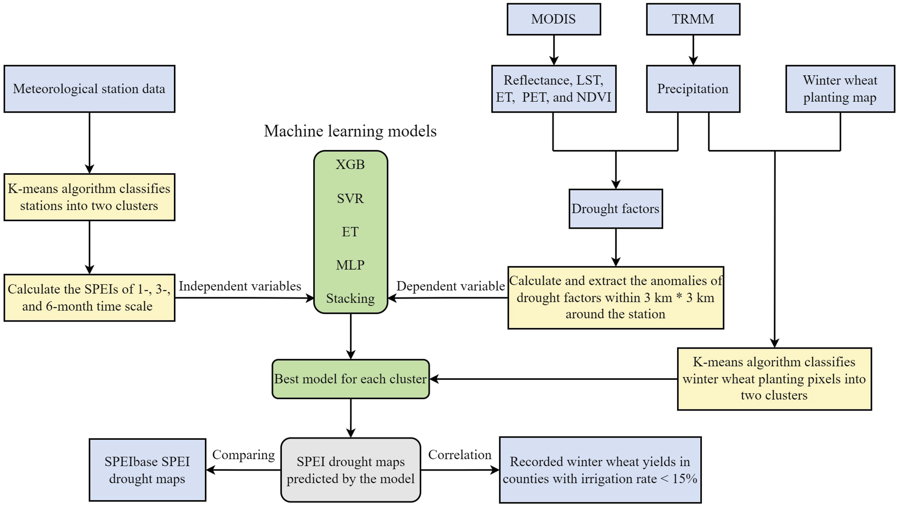

3.2 Machine learning algorithms

3.2.1 Extreme gradient boosting

XGB is an enhanced gradient boosting method, which implements an ensemble of boosted decision trees (Chen and Guestrin, 2016). The model continuously generates trees through feature splitting, and each new tree fits the residual of the previous tree to improve performance. Since XGB carries on the second order Taylor expansion to the loss function, it can usually achieve higher accuracy and lower overfitting risk. Furthermore, similar to Random Forests (RF), XGB supports random sampling of data on each node.

3.2.2 Support vector regression

SVR is used to solve regression issues (Cortes and Vapnik, 1995). Different from linear regression, SVR can tolerate a certain deviation between f(x) and y, and if the training sample falls within this deviation range, it is considered to be correct. For nonlinear data, SVR firstly finishes the computation in low-dimensional space, next implicitly translates the input space to the high-dimensional feature space using the kernel trick, and ultimately builds the ideal separation hyperplane, so resolving the linear inseparability issue in the initial space. In this study, we used a polynomial kernel.

3.2.3 Extra trees

ET is a variant of RF that combines a series of decision trees trained by all samples (Geurts et al., 2006). Random Forests often selects an optimal bifurcation value to divide the decision tree based on a certain principle. But ET chooses the bifurcation value in a completely random way, thus realizing the bifurcation of the decision tree. Therefore, although the same training sample set is used to build the decision trees and forecast, the model can still get completely different forecasts. This stronger randomness than RF may help to train better models.

3.2.4 Multi-layer perceptron

As an artificial neural network that feeds forward, MLP is composed of multi-layer nodes (Murtagh, 1991). A typical MLP consists of three layers: an input layer, several hidden layers, and an output layer. The number of neurons in the input and output layer is the same as the number of input and output variables, and the number of neurons in the hidden layer and the number of layers need to be determined by testing. The perceptron of the hidden layer is coupled to the units of the input layer and output layer through weight.

3.2.5 Development of ensemble model

We developed an ensemble model with the expectation of improving the predictive performance and robustness of a single model. Specifically, the ensemble of four machine learning algorithms (i.e., XGB, SVR, ET, and MLP) was realized through the Stacking regression model proposed by Wolpert (1992). The workflow of Stacking was shown in Figure 3. The framework of the model can be divided into two levels: firstly, training data for the meta-model was created by applying the divided training data to each base learner using ten-fold cross-validation. The test data were utilized to generate 10 predictions by each base learner at the above phase, and the average of those predictions served as the testing dataset for the meta-model. The new dataset was fed into the meta-model to get the final predictions. It should be mentioned that the linear regression was chosen as the meta-model to prevent overfitting brought on by sparse data. The development of four machine learning algorithms and Stacking models was realized by the “scikit-learn” package coded in Python language.

Figure 3.

Overall framework of Stacking.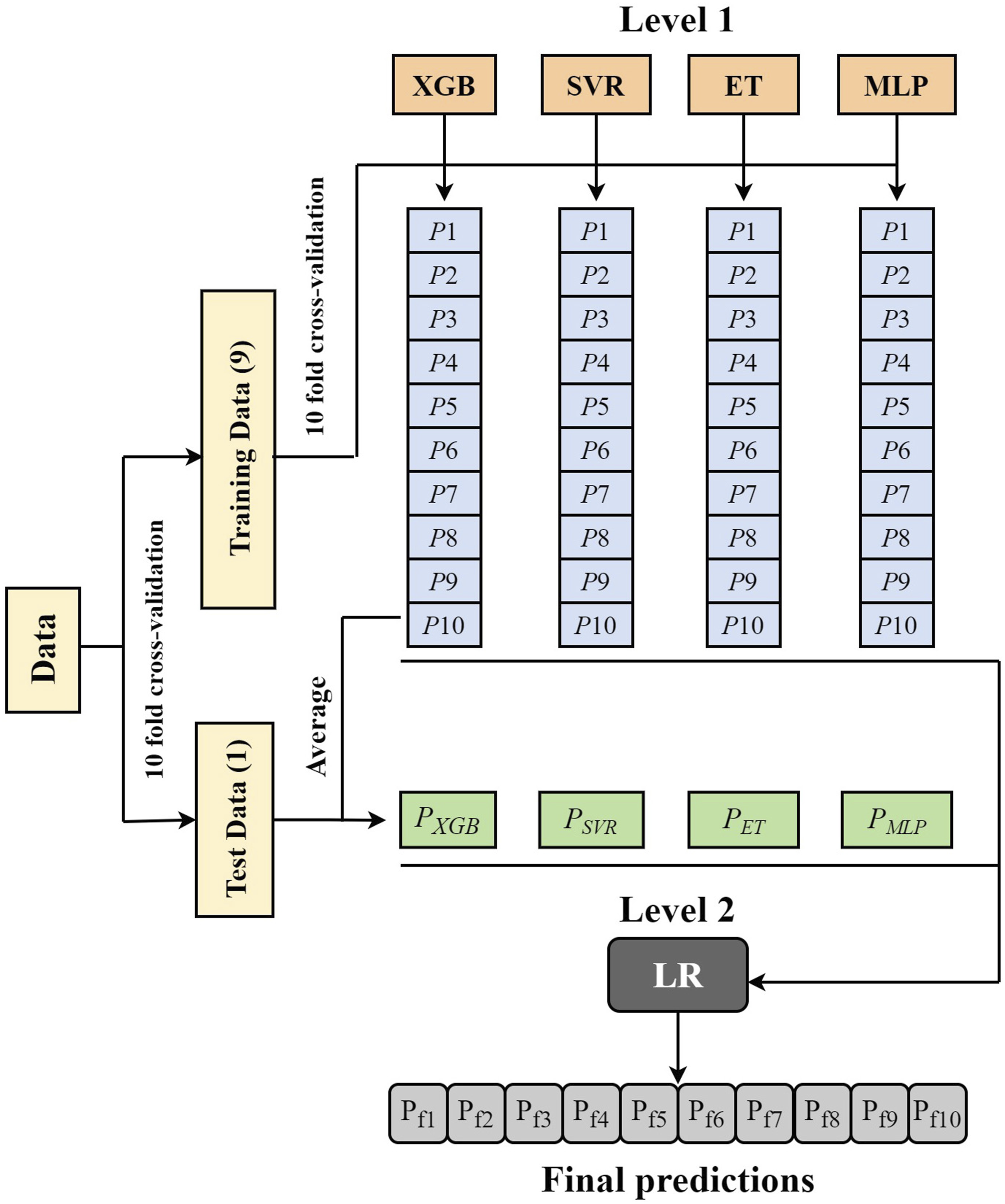

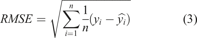
3.2.6 Model performance assessment

The grid search approach combined with ten-fold cross-validation was utilized to adjust the hyperparameters of the models to optimize their predictive performance. In this study, the models’ performance was assessed using the coefficient of determination (R²) and root mean square error (RMSE):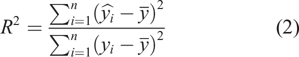

R^{2} = \frac{\sum_{i = 1}^{n} {(\hat{y_{i}} - \bar{y})}^{2}}{\sum_{i = 1}^{n} {(y_{i} - \bar{y})}^{2}}

(2)

R M S E = \sqrt{\sum_{i = 1}^{n} \frac{1}{n} (y_{i} - \hat{y_{i}})}

(3)

where n is the total number of samples,

y_{i}

and

\hat{y_{i}}

represent the station-based observed SPEI and predicted SPEI of sample i, respectively,

\bar{y}

is the average of the observations. Furthermore, we performed “leave-one-station-out” to evaluate the spatial generalization ability of the models, and accuracy metrics derived from cross-validation were utilized to assess the accuracy of prediction.

3.3 Drought trend analysis

The Mann-Kendall (MK) method, proposed by Mann (1945) and explained by Kendall (1990), is a nonparametric test that is frequently utilized to determine if time series contain trends (Hossain et al., 2014; Nalley et al., 2012). However, the prevalent autocorrelation in climate series can affect the analysis of trends to some extent (Wang et al., 2017). In this study, a trend-free pre-whitening MK (TFPW-MK) test proposed by Yue et al. (2002) was used to eliminate the interference of autocorrelation and track the increasing and decreasing trends of SPEI at the pixel level in the study regions in 2001 to 2017. The magnitude of the drought trend was determined by Sen’s slope estimator (Sen, 1968), with positive and negative values of slope indicating increasing and decreasing trends in drought, respectively. Furthermore, the p-value was used to reflect the significant level of drought changes.

IV Results

4.1 Model performance evaluation

The datasets of all stations and the corresponding stations of each cluster were utilized to assess the predictive accuracy of the models, respectively. The results of the accuracy metrics are shown in Figure 4. In general, ET outperformed other base learners (0.71∼0.77 in R² and 0.48∼0.53 in RMSE). Stacking enabled the highest prediction accuracy, with R² varying between 0.72 and 0.77 and RMSE of 0.47 to 0.52. For the three time scale SPEIs, the estimation accuracy of 1-month SPEI was slightly higher than that of 3-month and 6-month SPEIs. Furthermore, all the models had higher accuracy in cluster 1 (drier stations). Except for SVR, the other models fared equally in cluster 2 (wetter stations) and all stations, but SVR performed better in cluster 2.

Figure 4.

Accuracy of the machine learning models (i.e., XGB, SVR, ET, MLP, and Stacking) for predicting 1-, 3-, and 6-month SPEIs validated with the datasets of all stations and the corresponding stations of each cluster. (a) SPEI 1, (b) SPEI 3, (c) SPEI 6.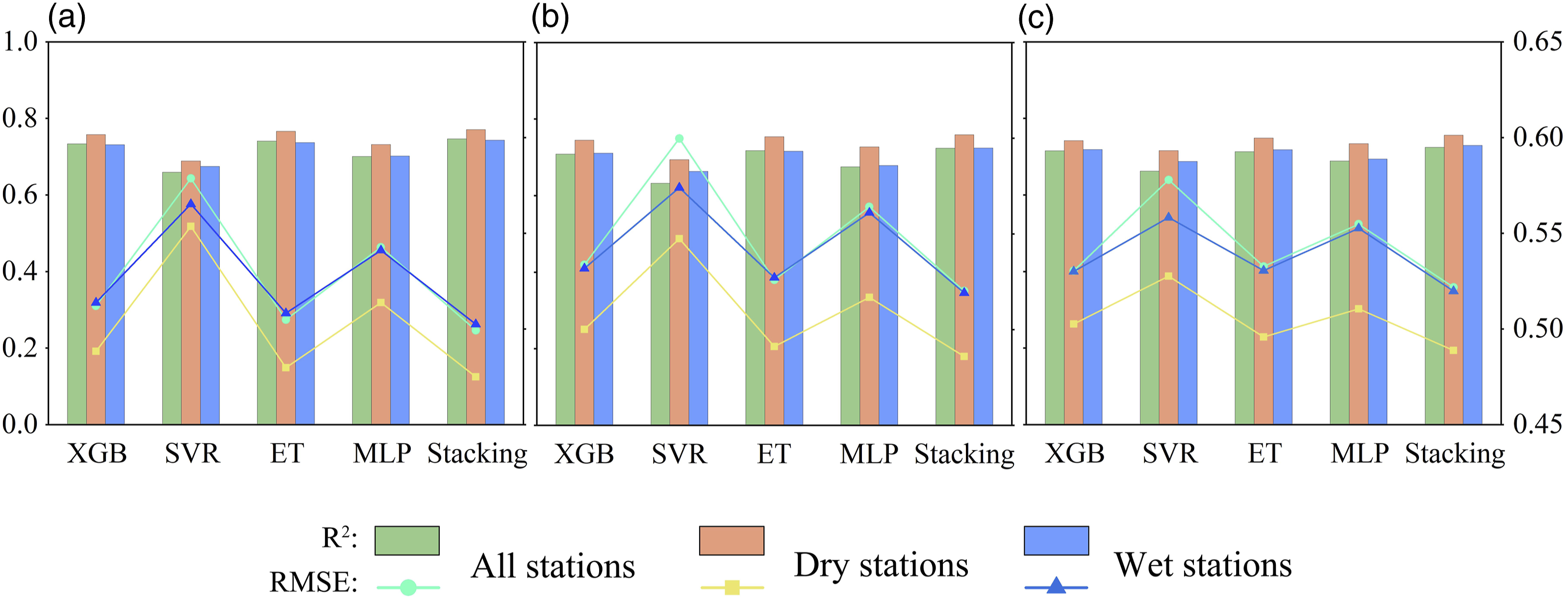

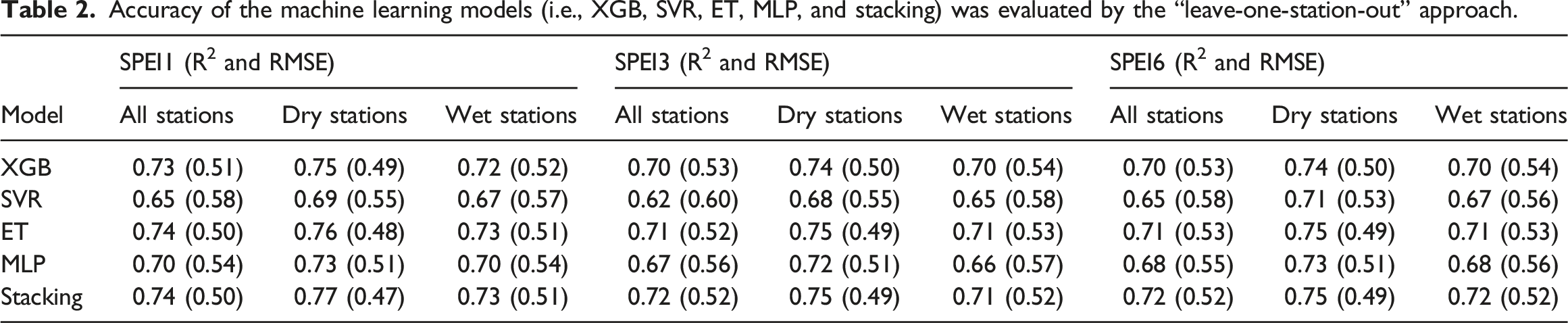
We carried out a “leave-one-station-out” experiment on the datasets of all stations and the corresponding stations of each cluster to evaluate the spatial generalization ability of each model (Table 2). Consistent with the results above, all models performed best in cluster 1 (drier stations). Except that SVR performed better in predicting 6-month SPEI, the estimation accuracy of other models for 1-month SPEI was higher than that of 3-month and 6-month SPEIs. The predictive performance of Stacking was superior to other models under any conditions, with R² ranged from 0.71 to 0.77 and RMSE ranged from 0.47 to 0.52. Therefore, the spatial generalization capability of Stacking is satisfactory and could be popularized in different regions.

Table 2.

Accuracy of the machine learning models (i.e., XGB, SVR, ET, MLP, and stacking) was evaluated by the “leave-one-station-out” approach.

Model	SPEI1 (R² and RMSE)			SPEI3 (R² and RMSE)			SPEI6 (R² and RMSE)
Model	All stations	Dry stations	Wet stations	All stations	Dry stations	Wet stations	All stations	Dry stations	Wet stations
XGB	0.73 (0.51)	0.75 (0.49)	0.72 (0.52)	0.70 (0.53)	0.74 (0.50)	0.70 (0.54)	0.70 (0.53)	0.74 (0.50)	0.70 (0.54)
SVR	0.65 (0.58)	0.69 (0.55)	0.67 (0.57)	0.62 (0.60)	0.68 (0.55)	0.65 (0.58)	0.65 (0.58)	0.71 (0.53)	0.67 (0.56)
ET	0.74 (0.50)	0.76 (0.48)	0.73 (0.51)	0.71 (0.52)	0.75 (0.49)	0.71 (0.53)	0.71 (0.53)	0.75 (0.49)	0.71 (0.53)
MLP	0.70 (0.54)	0.73 (0.51)	0.70 (0.54)	0.67 (0.56)	0.72 (0.51)	0.66 (0.57)	0.68 (0.55)	0.73 (0.51)	0.68 (0.56)
Stacking	0.74 (0.50)	0.77 (0.47)	0.73 (0.51)	0.72 (0.52)	0.75 (0.49)	0.71 (0.52)	0.72 (0.52)	0.75 (0.49)	0.72 (0.52)

4.2 The relative importance of remote sensing drought factors

The ET model can determine the importance of variables based on the contribution of each variable to the model’s prediction (Zhang et al., 2022b). We estimated remotely-sensed drought factors’ importance for predicting 1-, 3-, and 6-month SPEIs by the ET model based on the datasets of all stations and the corresponding stations of each cluster, respectively (Figure 5). Overall, three time scales Pre and LST (i.e., LSTd, LSTn, and LSTm) were more important than other predictive variables. Pre and LST with the same time scale as SPEI were generally ranked relatively high. Especially for Pre with the same time scale as SPEI, its relative importance was above 35%, while that of other variables was less than 10%, suggesting that precipitation was a key factor affecting regional meteorological drought. It is worth noting that for the three time scale SPEIs, Pre at the corresponding timescale was more important in relatively wet stations than in relatively dry stations. Compared with meteorological drought factors, the relative importance of vegetation drought factors (i.e., NDVI, NDDI, NDWI, and NMDI) was generally lower. In addition, NDDI7 was the most important vegetation drought factor in the prediction of three time scale SPEIs.

Figure 5.

The importance of remotely-sensed drought factors for predicting 1-, 3-, and 6-month SPEIs determined by the ET model based on datasets from all stations and the corresponding stations of each cluster. The “1,” “3,” and “6” suffixes to the variable names represent 1-, 3- and 6-month time scale means. The results of different time scale SPEIs for each dataset were normalized so that the sum was 100%. (a) SPEI 1, (b) SPEI 3, (c) SPEI 6.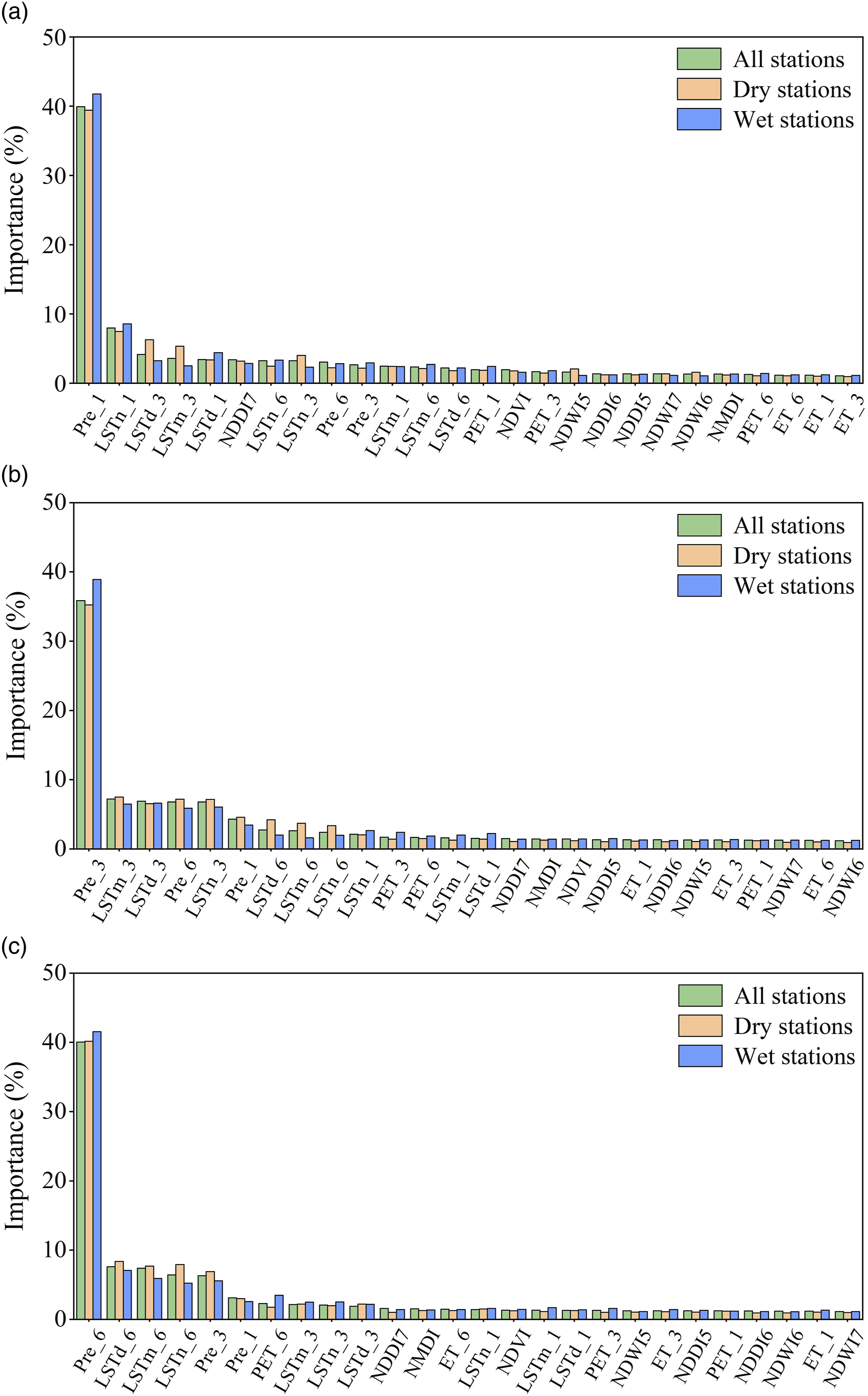

4.3 Comparison with SPEIbase maps

Stacking was shown to be the best model for predicting meteorological drought based on the models’ validation findings. Then, we used the Stacking model to predict the monthly spatial distribution maps of 1-, 3-, and 6-month SPEI to monitor the drought in winter wheat-growing areas from 2001 to 2017. In addition, the Global SPEI database (SPEIbase) provides monthly SPEI maps on multiple time scales with 0.5° spatial resolution based on monthly precipitation and potential evapotranspiration data from the Climate Research Unit (CRU) (Vicente-Serrano et al., 2010a, 2010b). To evaluate the drought maps obtained in this study, they were compared with the SPEI maps of SPEIbase on the same time scale.

4.3.1 Performance of monitoring agricultural drought

Considering that artificial measures such as irrigation could lessen crops’ sensitivity to drought conditions, we used the irrigation rate data provided by FAO (https://www.fao.org/aquastat/en/) to extract counties with irrigation rates less than 15% to focus on winter wheat grown under low irrigation density. Detrended winter wheat yields of these counties from 2002 to 2015 were used to evaluate SPEI drought maps’ capability to track agricultural drought. We calculated the average values of the monthly SPEI drought map derived from Stacking and SPEIbase for the winter wheat planting grids in these counties during the winter wheat-growing season, and then reflected their correlation with the detrended yields by Pearson’s correlation coefficient (Figure 6). The results show that the longer the time scale of SPEI, the greater the influence of SPEI on yields. Since 6-month SPEI had the highest correlation with detrended yields (r = 0.31), it was used for subsequent comparison and drought analysis. In addition, compared to SPEIs provided by SPEIbase, three time scale SPEIs predicted by Stacking had a marginally higher correlation with detrended yields.

Figure 6.

Scatterplots between detrended winter wheat yields and detrended SPEI values (from Stacking and SPEIbase) for counties with irrigation rates less than 15% throughout the wheat-growing season from 2002 to 2015. (a) SPEI 1, (b) SPEI 3, (c) SPEI 6.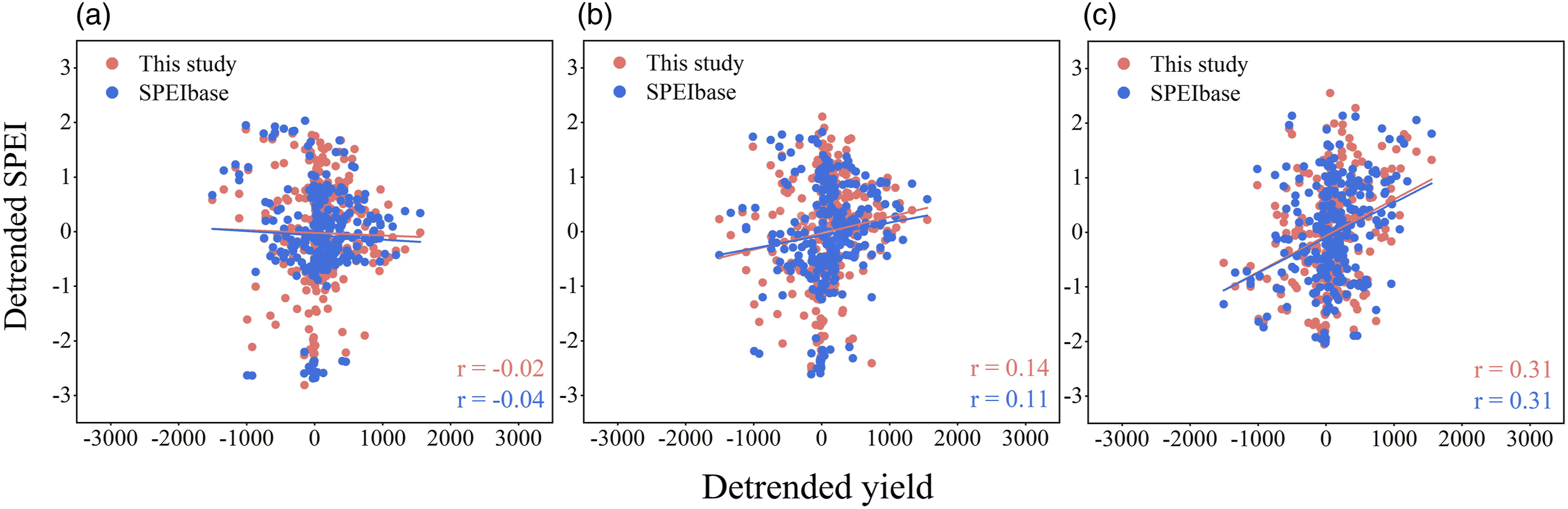

In addition, we explored and compared the predictive effectiveness of two types of SPEI maps with three time scales for winter wheat yield. Specifically, the mean SPEI values of winter wheat-growing regions in each county were calculated as input variables for the better performing models (i.e., XGB, ET, and Stacking), and model accuracy was validated based on a ten-fold cross-validation approach. The results showed that the prediction models using three time scales of SPEI indicators were able to capture winter wheat yield variation well (Figure 7). For the ET and Stacking models, the accuracy of the SPEI maps generated by Stacking outperformed the SPEI maps provided by SPEIbase. The best prediction accuracy was achieved by the Stacking model based on the Stacking SPEI map, explaining 69% of the yield variation with an RMSE of 724 kg/ha.

Figure 7.

The accuracy of three machine learning models predicting winter wheat yield using SPEI maps generated by Stacking and SPEIbase data set, respectively.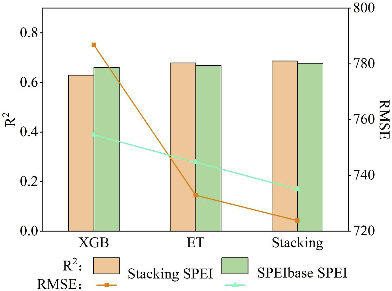

4.3.2 Drought monitoring performance in a typical dry growing season

Taking a typical dry growing season as an example, the monthly 6-month SPEI drought maps derived from Stacking and SPEIbase were compared. We calculated and ranked station-based average precipitation for each growing season (Figure S1). The growing season of 2011 (i.e., October 2010 to June 2011) had the lowest precipitation, so it was selected to display two types of SPEI drought maps (Figure 8). The findings demonstrate that the spatial distribution of the drought maps predicted by Stacking is generally similar to that of SPEIbase. The spatial correlation coefficients ranged from 0.26 to 0.87, with an average of 0.59, indicating a significant correlation between the two types of drought maps. Furthermore, both types of drought maps captured a wide range of 6-month time scale drought events from March to June, but SPEIbase showed more extreme drought conditions. The severity of drought episodes presented by both types of drought maps peaked in April and moderated in May and June. By calculating the mean of 6-month SPEI of all stations in the research regions, the results from March to June were −1.36, −1.89, −1.15, and −0.84, respectively, which were consistent with the spatial pattern of the drought maps.

Figure 8.

Comparison of monthly SPEI drought maps on 6-month time scale derived from Stacking and SPEIbase from October 2010 to June 2011. The spatial correlation (Pearson’s correlation coefficient) between the two types of drought maps was annotated on Stacking’s drought map for each month.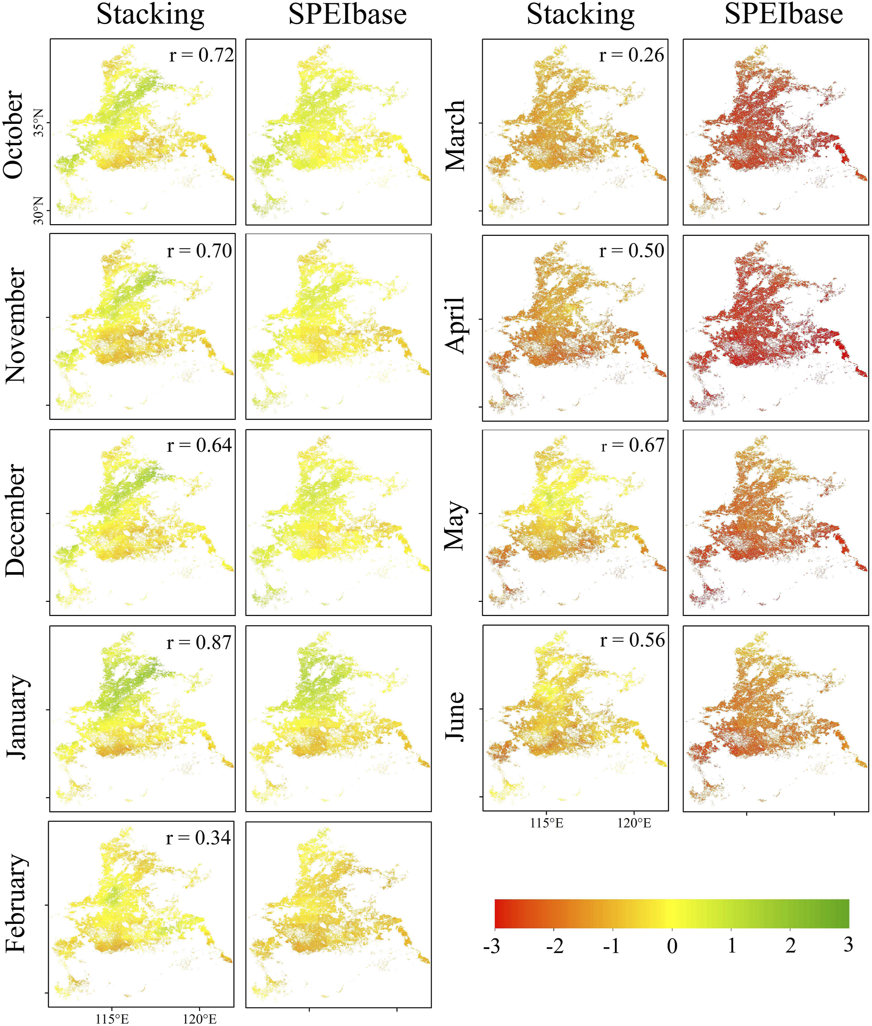

4.4 Drought trend for each month of the growing season

The TFPW-MK method was applied to analyze the trend of 6-month time scale drought maps predicted by Stacking for each month of the growing season (Figure 9). The spatial pattern and corresponding significant level of drought trend from 2001 to 2017 indicates the drought increased in the central part of the study region from October to December, especially the winter wheat planting area in eastern Henan Province, which experienced a significant drought trend (p-value ≤.05). The study area in May had varying degrees of a drought trend, with the northern of the research regions, specifically the south of Hebei Province and the northwest of Shandong Province, experiencing a marked increase in the severity of the drought. However, there was no discernible drought trend in the southern of the study region during the growing season.

Figure 9.

Spatial pattern of drought trend for the Stacking-predicted 6-month time scale drought maps from 2001 to 2017. The p-value represents the significant level of the trend.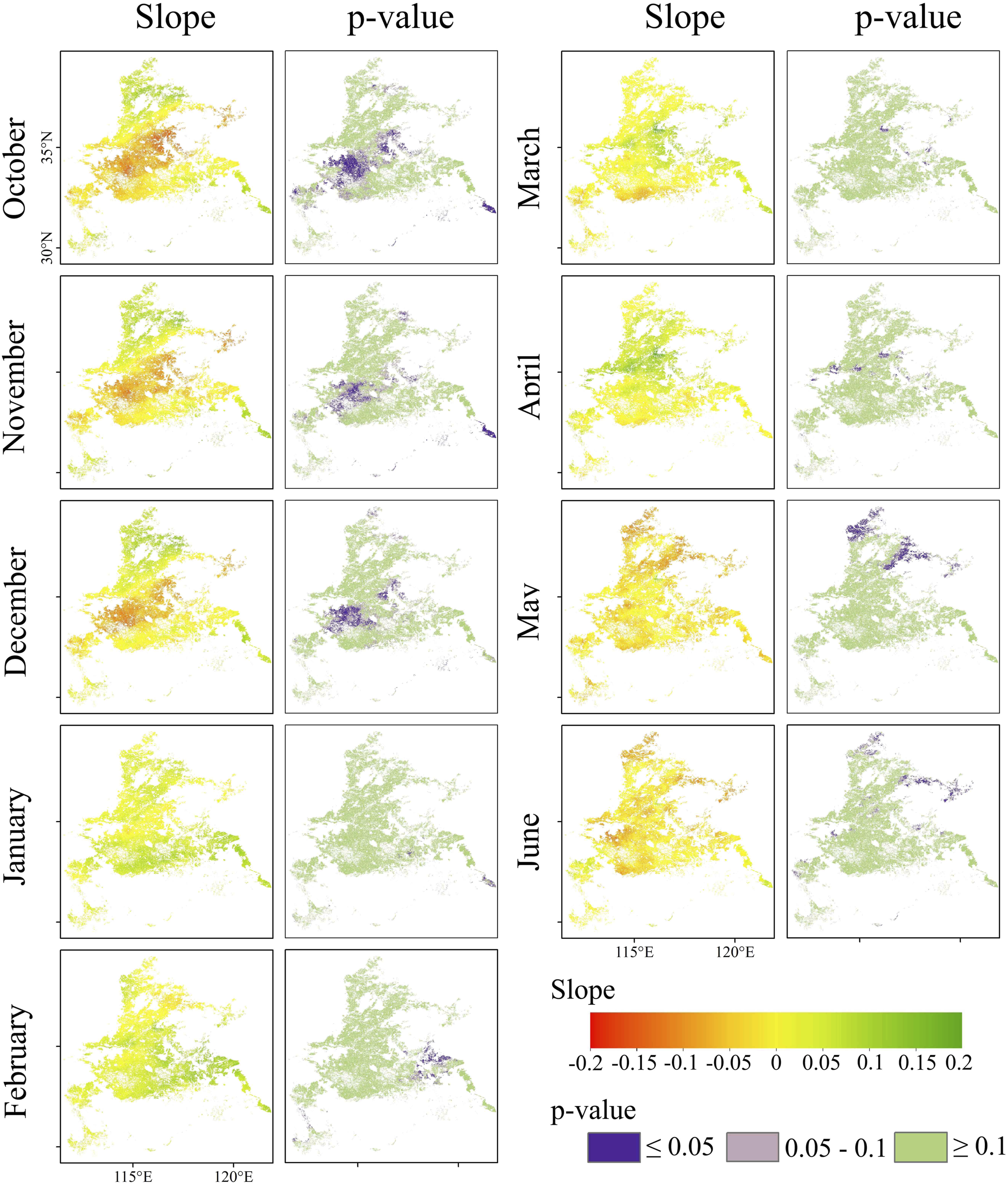

V Discussion

This study evaluated the applicability of an ensemble model based on remotely-sensed drought factors for drought monitoring in major winter wheat-growing regions of China. Through ten-fold cross-validation, it is concluded that the estimation accuracy of meteorological drought (i.e., SPEI) of the Stacking ensemble model was better than that of other models, with R² > 0.72 and RMSE between 0.47 and 0.52 (Figure 4). Due to the unbalanced properties of the model and the interaction between factors, it is frequently challenging for a single model to preserve robust predictive accuracy when variables with different characteristics are used as inputs (Feng et al., 2020; Lazaridis et al., 2011). For instance, the results of Alizadeh and Nikoo (2018) reported that the MLP model outperformed the other four models for drought estimates in Iran, which conflict with those of Feng et al. (2019) and this study. Therefore, it is crucial to increase the model’s robustness to make it suitable for drought prediction in different regions. Stacking is an ensemble approach that combines the strengths of various models and compensates for the shortcomings of just one model (Zhang et al., 2022b). In this study, selected heterogeneous models were integrated as base learners for the Stacking model to learn the advantages of each base learner for better results. In addition, Stacking also showed the best performance in the results of the “leave-one-station-out” experiment, with R² > 0.71 and RMSE between 0.47 and 0.52 (Table 2), indicating that Stacking had strong robustness at different stations and can be applied to meteorological drought monitoring in different regions. The prediction accuracy of all five machine learning models for 1-month SPEI was higher than that for 3- and 6-month SPEIs (Figure 4 and Table 2), which may be due to the shorter lag time of vegetation response to climate factors in the study region, so that vegetation-related drought factors contain more information about short-term climate change. The predictive performance of machine learning models varied by cluster, with all models estimating drought conditions more accurately for cluster 1 than for cluster 2 and for all stations (Figure 4 and Table 2). Because the stations of cluster 1 are located in a relatively dry environment and those of cluster 2 is in a relatively humid environment, the models developed in this study performed better in more arid regions, which is consistent with the findings of Park et al. (2016).

The ET model with the highest estimation accuracy in the ensemble was applied to evaluate the importance of 26 drought factors (Figure 5), which used the increase of the mean square error (MSE) caused by randomly arranging the selected variables in the out-of-bag sample to represent the relative importance of variables. As found by Feng et al. (2019) and Park et al. (2016), precipitation at the same time scale was the most important drought factor when estimating SPEI, and its relative importance was higher in relatively humid regions than in relatively arid regions. The relative importance of evapotranspiration-related variables (i.e., ET and PET) was relatively low, which is comparable to the results of Zhang et al. (2022a). Vegetation drought factors monitor drought by representing vegetation water content (Zhou et al., 2017), and the reason for their lower relative importance may be that these factors contain more information on drought-related biophysical processes than on meteorological drought (Rhee et al., 2010). Similar to the results of Zhang et al. (2022a), NDDI7 was the most important variable among all vegetation drought factors, especially for 1-month SPEI, which means that it may be more sensitive to reflect the reaction of vegetation to drought.

Monthly spatial distribution maps of 1-, 3-, and 6-month SPEIs were derived from the Stacking model and compared with the SPEI maps of SPEIbase at the corresponding time scale. Drought events have negative effects on the normal growth of crops by reducing the available water content and photosynthesis of crops and ultimately lead to lower yields (Iqbal et al., 2020; Ray et al., 2018). Therefore, this study used detrended yields to assess the suitability of SPEI maps for monitoring agricultural drought. The results of correlation show that the drought maps derived from Stacking and SPEIbase had similar correlations with yield (Figure 6). Shorter time scale SPEIs (i.e., 1- and 3-month SPEIs) were less correlated with yield, which may be attributed to the adaptability of crops to short-term water deficit, making short-term drought stress less impactful on yields (Abid et al., 2016; Chenu et al., 2011; Mu et al., 2021). For winter wheat in the study area, 6-month SPEI may be a better indicator for agricultural drought monitoring, and it can also be used as an independent variable to predict yield. The comparison of 6-month SPEI drought maps derived from Stacking and SPEIbase in a typical dry growing season shows that the spatial patterns of the two types of drought maps were highly similar in most cases, with a mean spatial correlation of 0.59. The spatial resolution of Stacking-predicted SPEI drought maps is 1 km, which is higher than that of SPEIbase-provided SPEI drought maps, so more spatial information about drought can be displayed. Figure 8 shows that both types of drought maps successfully captured the drought events on the 6-month time scale from March to June 2011, and their change processes were consistent with the station-based SPEI. Therefore, the ensemble model integrating multiple remotely-sensed drought factors is worthy to be applied to regional drought monitoring. In addition, the drought trend in the central of the study area from October to December and the northern part of the study area in May needs to be watched and guarded against. Irrigation and the adoption of drought-resistant winter wheat varieties are both effective measures to deal with drought risk (Hervás-Gámez and Delgado-Ramos, 2019; Zhang et al., 2016). No apparent drought trend was observed in the south of the research regions, which might be because of plentiful precipitation in this region and the less risk of suffering from drought.

VI Conclusion

In this study, the performance of four common machine learning algorithms (i.e., XGB, SVR, ET, and MLP) and an ensemble learning method (i.e., Stacking) to estimate station-based meteorological drought indicators (i.e., 1-, 3-, and 6-month SPEIs) in the case of integrating multiple remotely-sensed drought factors were explored. Furthermore, county-level winter wheat yield records and the drought maps provided by SPEIbase were used to evaluate the ability of SPEI drought maps predicted by Stacking in monitoring agricultural drought. The results show that the Stacking model, which integrated four machine learning models, achieved the best forecasting ability and generalization capability, and performed better in relatively dry regions than in relatively wet regions. By evaluating the SPEI drought maps with a resolution of 1 km predicted by the Stacking model, it is concluded that the correlation between 6-month SPEI and detrended yield was higher than that between 1- and 3-month SPEIs and detrended yield, so 6-month SPEI is better suited for monitoring agricultural drought. In addition, Stacking-predicted drought maps successfully captured the spatial pattern and change process of drought events. The technical method suggested in this study could be applied to agricultural drought monitoring in other areas.

There are still some potential problems in the practice of agricultural drought in this study. For example, the resolution of the drought maps provided in this study is relatively coarse, so it is difficult to be used for drought monitoring at a finer scale (e.g., field scale). Improving spatial resolution can provide more spatial information on drought. Agricultural irrigation can effectively alleviate crop yield loss caused by drought, but the effect of irrigation was not considered in the SPEI. As irrigation measures affect the change of soil moisture, the application of the technical framework to the development of soil moisture-related indicators is the main approach to improving agricultural drought monitoring.

Supplemental Material

Supplemental Material - Ensemble learning based on remote sensing data for monitoring agricultural drought in major winter wheat-producing areas of China

Supplemental Material for Ensemble learning based on remote sensing data for monitoring agricultural drought in major winter wheat-producing areas of China by Lunche Wang, Yuefan Zhang, Xinxin Chen, Yuting Liu, Shaoqiang Wang and Lizhe Wang in Progress in Physical Geography: Earth and Environment

Footnotes

Declaration of conflicting interests

The author(s) declared no potential conflicts of interest with respect to the research, authorship, and/or publication of this article.

Funding

This work was financially supported by the National Natural Science Foundation of China (41975044, 41925007, and 41801021), Open Fund of Hubei Luojia Laboratory (No.2201000043) and Fundamental Research Founds for National University, China University of Geosciences, Wuhan.

ORCID iD

Lunche Wang

Supplemental Material

Supplemental material for this article is available online.

References

Abid

Tian

Ata-Ul-Karim

, et al. (2016) Adaptation to and recovery from drought stress at vegetative stages in wheat (Triticum aestivum) cultivars. Functional Plant Biology: FPB 43: 1159–1169.

Alizadeh

Nikoo

(2018) A fusion-based methodology for meteorological drought estimation using remote sensing data. Remote Sensing of Environment 211: 229–247.

Chen

Guestrin

(2016) XGBoost. In: Proceedings of the 22nd ACM SIGKDD international conference on knowledge discovery and data mining, London, 12th, July, pp. 785–794.

Chen

Wang

(2012) Statistical uncertainty estimation using random forests and its application to drought forecast. Mathematical Problems in Engineering 2012: 1–12.

Chenu

Cooper

Hammer

, et al. (2011) Environment characterization as an aid to wheat improvement: interpreting genotype–environment interactions by modelling water-deficit patterns in North-Eastern Australia. Journal of Experimental Botany 62: 1743–1755.

Cortes

Vapnik

(1995) Support-vector networks. Machine Learning 20: 273–297.

Tian

, et al. (2013) A comprehensive drought monitoring method integrating MODIS and TRMM data. International Journal of Applied Earth Observation and Geoinformation 23: 245–253.

Feng

Wang

Liu

, et al. (2019) Machine learning-based integration of remotely-sensed drought factors can improve the estimation of agricultural drought in South-Eastern Australia. Agricultural Systems 173: 303–316.

Feng

Zhang

, et al. (2020) Alfalfa yield prediction using UAV-based hyperspectral imagery and ensemble learning. Remote Sensing 12: 2028.

10.

Gang

(2002) Several issues on aridification in the northern China. Climatic and Environmental Research. 7(1): 22–29.

11.

Gao

B-C

(1996) NDWI—a normalized difference water index for remote sensing of vegetation liquid water from space. Remote Sensing of Environment 58: 257–266.

12.

Geurts

Ernst

Wehenkel

(2006) Extremely randomized trees. Machine Learning 63: 3–42.

13.

Brown

Verdin

, et al. (2007) A five-year analysis of MODIS NDVI and NDWI for grassland drought assessment over the central great plains of the United States. Geophysical Research Letters 34: L06407.

14.

Hartigan

Wong

(1979) Algorithm as 136: a K-means clustering algorithm. Applied Statistics 28: 100–108.

15.

Hervás-Gámez

Delgado-Ramos

(2019) Drought management planning policy: from Europe to Spain. Sustainability 11: 1862.

16.

Hossain

Roy

Datta

(2014) Spatial and temporal variability of rainfall over the south-west coast of Bangladesh. Climate 2: 28–46.

17.

Lin

, et al. (2010) Emergy assessment of a wheat-maize rotation system with different water assignments in the north China plain. Environmental Management 46: 643–657.

18.

Iqbal

Singh

Ansari

(2020) Effect of drought stress on crop production. New Frontiers in Stress Management for Durable Agriculture. Singapore: Springer.

19.

Jiang

Xie

, et al. (2015) Use of four drought indices for evaluating drought characteristics under climate change in Shaanxi, China: 1951–2012. Natural Hazards 75: 2885–2903.

20.

Kendall

(1990) Rank correlation methods. British Journal of Psychology 25: 86–91.

21.

Lazaridis

Verbesselt

Robinson

(2011) Penalized regression techniques for prediction: a case study for predicting tree mortality using remotely sensed vegetation indices. Canadian Journal of Forest Research 41: 24–34. This article is one of a selection of papers from extending forest inventory and monitoring over space and time.

22.

Yang

Davey-Rothwell

, et al. (2016) Hydrological drought class transition using SPI and SRI time series by loglinear regression. Water Resources Management 30: 669–684.

23.

Liu

Luo

Yang

, et al. (2015) Investigation of the probability of concurrent drought events between the water source and destination regions of China’s water diversion project. Geophysical Research Letters 42: 8424–8431.

24.

Carbone

Huang

, et al. (2020) Mapping the sensitivity of agriculture to drought and estimating the effect of irrigation in the United States, 1950–2016. Agricultural and Forest Meteorology 292–293: 108124.

25.

Luo

Zhang

Chen

, et al. (2020) ChinaCropPhen1km: a high-resolution crop phenological dataset for three staple crops in China during 2000–2015 based on leaf area index (LAI) products. Earth System Science Data 12: 197–214.

26.

Mann

(1945) Nonparametric tests against trend. Econometrica 13: 245–259.

27.

McKee

Doesken

Kleist

(1993) The relationship of drought frequency and duration to time scales. In: Proceedings of the 8th conference on applied climatology, Anaheim, CA, 17–22 January 1993, pp. 179–183.

28.

Mokhtar

Jalali

, et al. (2021) Estimation of SPEI meteorological drought using machine learning algorithms. IEEE Access 9: 65503–65523.

29.

Cai

Sun

, et al. (2021) The physiological response of winter wheat under short-term drought conditions and the sensitivity of different indices to soil water changes. Agricultural Water Management 243: 106475.

30.

Murtagh

(1991) Multilayer perceptrons for classification and regression. Neurocomputing 2: 183–197.

31.

Nalley

Adamowski

Khalil

(2012) Using discrete wavelet transforms to analyze trends in streamflow and precipitation in Quebec and Ontario (1954–2008). Journal of Hydrology 475: 204–228.

32.

Nicholls

Neville (1997) Increased Australian wheat yield due to recent climate trends. Nature 387: 484–485.

33.

Palmer

(1965) Meteorological Drought. New York: US Department of Commerce, Weather Bureau.

34.

Park

Jang

, et al. (2016) Drought assessment and monitoring through blending of multi-sensor indices using machine learning approaches for different climate regions. Agricultural and Forest Meteorology 216: 157–169.

35.

Potopová

Štěpánek

Možný

, et al. (2015) Performance of the standardised precipitation evapotranspiration index at various lags for agricultural drought risk assessment in the Czech republic. Agricultural and Forest Meteorology 202: 26–38.

36.

Quiring

Ganesh

(2010) Evaluating the utility of the Vegetation Condition Index (VCI) for monitoring meteorological drought in Texas. Agricultural and Forest Meteorology 150: 330–339.

37.

Ray

Fares

Risch

(2018) Effects of drought on crop production and cropping areas in Texas. Agricultural & Environmental Letters 3: 170037.

38.

Rhee

Carbone

(2010) Monitoring agricultural drought for arid and humid regions using multi-sensor remote sensing data. Remote Sensing of Environment 114: 2875–2887.

39.

Rouse

Jr. Haas

Schell

, et al. (1974) Monitoring vegetation systems in the great plains with erts. 309, London.

40.

Sen

(1968) Estimates of the regression coefficient based on Kendall’s Tau. Journal of the American Statistical Association 63: 1379–1389.

41.

Sun

Zhang

Wen

, et al. (2017) Multisource data-based integrated agricultural drought monitoring in the Huai river basin, China. Journal of Geophysical Research: Atmospheres 122: 10751–10772.

42.

Swain

Wardlow

Narumalani

, et al. (2011) Assessment of vegetation response to drought in Nebraska using terra-MODIS Land surface temperature and normalized difference vegetation index. GIScience and Remote Sensing 48: 432–455.

43.

Thornthwaite

(1948) An approach toward a rational classification of climate. Geographical Review 38: 55–94.

44.

Tian

Yuan

Quiring

(2018) Evaluation of six indices for monitoring agricultural drought in the south-central United States. Agricultural and Forest Meteorology 249: 107–119.

45.

Touma

Ashfaq

Nayak

, et al. (2015) A multi-model and multi-index evaluation of drought characteristics in the 21st century. Journal of Hydrology 526: 196–207.

46.

Vicente-Serrano

Beguería

López-Moreno

(2010a) A multiscalar drought index sensitive to global warming: the standardized precipitation evapotranspiration index. Journal of Climate 23: 1696–1718.

47.

Vicente-Serrano

Beguería

López-Moreno

, et al. (2010b) A new global 0.5° gridded dataset (1901–2006) of a multiscalar drought index: comparison with current drought index datasets based on the palmer drought severity index. Journal of Hydrometeorology 11: 1033–1043.

48.

Vicente-Serrano

Beguería

Lorenzo-Lacruz

, et al. (2012) Performance of drought indices for ecological, agricultural, and hydrological applications. Earth Interactions 16: 1–27.

49.

Wang

(2007) NMDI: a normalized multi-band drought index for monitoring soil and vegetation moisture with satellite remote sensing. Geophysical Research Letters 34: L20405.

50.

Wang

Vicente-serrano

Tao

, et al. (2016) Monitoring winter wheat drought threat in Northern China using multiple climate-based drought indices and soil moisture during 2000–2013. Agricultural and Forest Meteorology 228–229: 1–12.

51.

Wang

Lai

, et al. (2017) Does drought in China show a significant decreasing trend from 1961 to 2009? Science of the Total Environment 579: 314–324.

52.

Wilhite

(2000) Drought as a natural hazard: concepts and definitions. Drought a Global Assessment: 57–64. Beijing.

53.

Wilhite

Glantz

(1985) Understanding: the drought phenomenon: the role of definitions. Water International 10: 111–120.

54.

Wolpert

(1992) Stacked generalization. Neural Networks 5: 241–259.

55.

Zhang

C-Y

, et al. (2019) Modified palmer drought severity index: model improvement and application. Environment International 130: 104951.

56.

Yue

Pilon

Phinney

, et al. (2002) The influence of autocorrelation on the ability to detect trend in hydrological series. Hydrological Processes 16: 1807–1829.

57.

Zhang

Jia

(2013) Monitoring meteorological drought in semiarid regions using multi-sensor microwave remote sensing data. Remote Sensing of Environment 134: 12–23.

58.

Zhang

Han

Jia

, et al. (2016) Management of drought risk under global warming. Theoretical and Applied Climatology 125: 187–196.

59.

Zhang

Chen

, et al. (2017) Multi-sensor integrated framework and index for agricultural drought monitoring. Remote Sensing of Environment 188: 141–163.

60.

Zhang

Shi

Singh

, et al. (2022a) Droughts across China: drought factors, prediction and impacts. Science of the Total Environment 803: 150018.

61.

Zhang

Wang

Chen

, et al. (2022b) Prediction of winter wheat yield at county level in China using ensemble learning. Progress in Physical Geography: Earth and Environment 45: 676–696.

62.

Zhou

Fang

Wang

, et al. (2017) Quantifying agricultural drought in tallgrass prairie region in the U.S. southern great plains through analysis of a water-related vegetation index from MODIS images. Agricultural and Forest Meteorology 246: 111–122.

Supplementary Material

Please find the following supplemental material available below.

For Open Access articles published under a Creative Commons License, all supplemental material carries the same license as the article it is associated with.

For non-Open Access articles published, all supplemental material carries a non-exclusive license, and permission requests for re-use of supplemental material or any part of supplemental material shall be sent directly to the copyright owner as specified in the copyright notice associated with the article.

0.00 MB

0.17 MB