Computational fluid dynamics simulation and full-scale experimental model inter-comparison of the wind flow around a university campus

Abstract

In this article, results obtained from two computational fluid dynamics solvers, WindSim and OpenFOAM, have been compared for the wind flow around the University of Mauritius’ campus for different wind directions, and a reference incident wind speed at diverse height above ground level. A grid resolution study is performed for both software and the mean differences of the two solvers with multiple turbulence models (standard k-ε, k-ε with Yap correction, and renormalization group k-ε) are analyzed with onsite measured data. The article concludes that the best results for the computational fluid dynamics simulation of the wind flow around buildings are obtained using OpenFOAM with k-ε turbulence model including Yap correction.

Keywords

Urban region computational fluid dynamics simulations around buildings OpenFOAM WindSim

Introduction

The analysis of wind flow patterns in urban regions is necessary in order to locate ventilation, discomfort regions, as well as areas where wind energy can be harnessed (Houda et al., 2012; Toja-Silva et al., 2013). The history of wind flow over a particular area, as well as the wind interaction with surrounding buildings, has to be studied in detail. For instance, in order to more efficiently harness power, it is important to find the zones of vortices, wind recirculation, and turbulent wakes, as the building geometry does affect the flow of wind (Kalmikov et al., 2010; Toja-Silva et al., 2015b). As in situ measurements are not so obvious in urban areas where buildings are in close proximity to each other, a complete computational fluid dynamics (CFD) model at micro-scale level is the most suitable method of investigation (Britter and Hanna, 2003; Britter and Schatzmann, 2007). It is commonly known that wind activity is magnified at the foot of high-rise buildings and in canyons (Blocken et al., 2007). In particular, the flow near the ground shows drastic changes in speed and direction because of the intricate interaction between the wind and the buildings themselves (shapes, sizes, position, etc.). A brief review of the wind energy literature reveals that in recent years, there has been an increasing development of suitable numerical models for the analysis of urban wind flow patterns (Houda et al., 2012). Models for urban regions include a global analysis on the flow patterns of wind around the building shape and canyons, the placement of wind breakers for the comfort of pedestrians, and so on. Several vegetation canopy models proposed for the study of aerodynamic effects of trees are also found in the literature. Past studies have also shown a great interest in natural ventilation in urban areas. The works of Britter and Hanna (2003), Blocken et al. (2008), Van Hooff and Blocken (2010) are typical examples.

CFD has become more prominent in different fields over the past decades and increasingly popular for the analysis of urban wind flow patterns (Houda et al., 2012). It can be useful to estimate the effect of the wind near edifices, as different models can be chosen to take into consideration the impact of complicated building arrangements and shapes (Toja-Silva et al., 2015b). Many CFD studies have shown that a detailed wind map of urban areas is vital for the placement of wind turbines (Kalmikov et al., 2010). However, it can be exceedingly challenging in terms of computing resources to use a CFD model for such an endeavor. Hence, modelers need to find a balance between map resolution and available computational resources. Previously, the CFD study of the wind flow around localized buildings was limited to single isolated buildings (Hanson et al., 1986; Stathopoulos and Baskaran, 1996). Recently, due to the advent of more powerful computers, urban areas with increasingly complex building arrangements have been studied (Blocken and Carmeliet, 2002; Blocken and Carmeliet, 2004a; Blocken and Carmeliet, 2004b; Blocken et al., 2007). This subject has thoroughly been reviewed by Vardoulakis et al. (2003) and Li et al. (2006) summarizing recent advancements in the CFD modeling of wind field in street canyons. Further studies have analyzed the influence of parameters on the flow, for example, building geometry (Toja-Silva et al., 2015a), street dimensions and wind direction (McNabola et al., 2009; Sabatino et al., 2008), the closeness and packing density of the buildings (Sabatino et al., 2007), thermal stratification (Baik et al., 2007; Kang et al., 2008), vehicular motion (Kumar et al., 2008; Solazzo et al., 2007), flow between canyons (Blocken et al., 2008), and so on. For this endeavor, the use of geographical information systems (GIS) was favored for both rural and urban planning. Gagliano et al. (2013) provide a good overview on how to exploit wind flow in urban areas while using CFD codes with GIS software. It involves the merging of digital maps and geo-referenced data which explains clearly the position and shape including elevation and roughness factor of the area under consideration.

The present work focuses mainly on the comparison of results obtained using two CFD solvers, WindSim (Meissner, 2010) and OpenFOAM (2015), with the in situ measurements of wind data in a university campus, the University of Mauritius (UoM). The CFD commercial software WindSim and the open source package OpenFOAM were used to simulate the flow pattern over the campus with multiple turbulence models. In the next section, the mathematical model is described, followed by a brief presentation of the site under investigation. The experimental measurements and inlet wind conditions for the CFD models are then elaborated in the subsequent section, and the simulation results are commented in the following section. Finally, the major conclusions of this work are given.

The mathematical model

Governing equations and turbulence modeling

The fluid flow in the atmospheric boundary layer is governed by the Navier–Stokes equations, which are described in terms of mass and momentum conservation equations. In this work, the flow was assumed to be steady and turbulent. The velocity is denoted by $\vec{u} = {(u_{x}, u_{y}, u_{z})}^{T}$ , pressure by p, density by ρ, and fluid dynamic viscosity by µ. By decomposing the variables (say $ϕ (x_{i}, t)$ ) into mean value $\bar{ϕ} (x_{i})$ and an oscillating value $ϕ^{'} (x_{i}, t)$ (e.g. $u_{i} = {\bar{u}}_{i} + {u^{'}}_{i}$ , where i = x, y, or z) to describe turbulence effects, the Reynolds-Averaged Navier–Stokes (RANS) equations are obtained (equations (1) to (3) in tensor notation in Cartesian coordinates) (Ferziger and Peric, 2002; Wesseling, 2001)

\frac{\partial (ρ {\bar{u}}_{j})}{\partial x_{j}} = 0

(1)

\frac{\partial}{\partial x_{j}} (ρ {\bar{u}}_{i} {\bar{u}}_{j}) = - \frac{\partial \bar{p}}{\partial x_{i}} + \frac{\partial}{\partial x_{j}} [μ (\frac{\partial {\bar{u}}_{i}}{\partial x_{j}} + \frac{\partial {\bar{u}}_{j}}{\partial x_{i}}) - ρ \bar{u_{i}^{'} u_{j}^{'}}]

(2)

ρ \bar{u_{i}^{'} u_{j}^{'}} = \frac{2}{3} ρ δ_{i j} k - μ_{t} (\frac{\partial {\bar{u}}_{i}}{\partial x_{j}} + \frac{\partial {\bar{u}}_{j}}{\partial x_{i}})

(3)

where $δ_{i j}$ is the Kronecker symbol ( $δ_{i j} = 1$ if i = j, and $δ_{i j} = 0$ otherwise). Turbulence effects were modeled using the Standard k-ε transport equations which are formulated as follows

\frac{\partial}{\partial x_{j}} (ρ k {\bar{u}}_{j}) = \frac{\partial}{\partial x_{j}} [(\frac{μ_{t}}{σ_{k}}) \frac{\partial k}{\partial x_{j}}] + P_{k} - ρ ε

(4)

\frac{\partial}{\partial x_{j}} (ρ ε {\bar{u}}_{j}) = \frac{\partial}{\partial x_{j}} [(\frac{μ_{t}}{σ_{ε}}) \frac{\partial ε}{\partial x_{j}}] + C_{ε 1} P_{k} \frac{ε}{k} - ρ C_{ε 2} \frac{ε^{2}}{k}

(5)

where k is the turbulent kinetic energy, ε is the dissipation rate of kinetic energy, and $μ_{t}$ µ_t is the eddy viscosity which is expressed as

μ_{t} = ρ C_{μ} \frac{k^{2}}{ε}

(6)

where C_µ, $σ_{k}$ , $σ_{ε}$ , $C_{ε 1}$ , and $C_{ε 2}$ are constants that are defined in Table 1. The variable $P_{k}$ , which is the turbulent kinetic energy production, is given by

P_{k} = μ_{t} (\frac{\partial {\bar{u}}_{i}}{\partial x_{j}} + \frac{\partial {\bar{u}}_{j}}{\partial x_{i}}) \frac{\partial {\bar{u}}_{i}}{\partial x_{j}}

(7)

Table 1.

Constants for the turbulence models (Ferziger and Peric, 2002).

Model	$C_{μ}$	$σ_{k}$	$σ_{ε}$	$C_{ε 1}$	$C_{ε 2}$
Standard k-ε (including Yap correction)	0.09	1.00	1.30	1.44	1.92
RNG k-ε	0.08	0.72	0.72	1.42	1.68

RNG: renormalization group.

The Yap correction (Yap, 1987) consists of a modification of equation (5) by adding an extra source term $(ρ S_{ε})$ to the right of the equation, which can be written as

S_{ε} = 0.83 \frac{ε^{2}}{k} (\frac{k^{1.5}}{ε l_{ε}} - 1) {(\frac{k^{1.5}}{ε l_{ε}})}^{2}

(8)

where $l_{ε} = C_{μ}^{- 0.75} κ y_{n}$ , κ is the Von-Karman constant (equal to 0.41), and $y_{n}$ is the normal distance to the nearest wall.

Developed by Yakhot et al. (1992), the renormalization group (RNG) k-ε model renormalizes the Navier–Stokes equations by also adding a term (R) to the right hand side of the equation (5), which is given as

R = - \frac{ρ C_{μ} η^{3} (1 - \frac{η}{η_{0}})}{1 + β η^{3}} \frac{ε^{2}}{k}

(9)

where $η_{0} = 4.38$ , $β = 0.012$ , $η = S k / ε$ , and $S^{2} = 2 S_{i j} S_{i j}$ is the magnitude of the rate-of-strain. The values of all the constants are as given in Table 1.

WindSim and OpenFOAM

WindSim is a CFD software used to evaluate the wind resources of a site by solving the RANS equations with the finite-volume method. It is commercialized by the company WindSim AS, Norway. WindSim uses a core constituted by the general purpose CFD solver Phoenics (developed by Cham, UK) in an iterative way. It uses the General Collocated Velocity (GVC) solver which can handle highly non-orthogonal grids and secure convergence with included angles as small as 10°. The GVC method implements a block-structured multi-block especially designed to tackle highly non-orthogonal grids. A conjugate-residual linear solver with LU preconditioning is employed, and a segregated pressure based strategy with an additional correction of the cell centered momentum velocity is used. The second-order linear upwind interpolation (Central Difference Scheme) for divergence terms are used for the discretization of the differential operators. For more details about WindSim, the interested reader is referred to the work of Meissner (2010).

OpenFOAM is an open source finite-volume CFD library that includes many general purpose CFD solvers and libraries. Here, we use the simpleFoam solver to solve the RANS equations. The solver is based on the SIMPLE algorithm. For the spatial discretization of differential operators, Gaussian integration is used with different interpolation schemes. Second-order linear interpolation is used for gradient terms, second-order linear upwind interpolation for divergence terms, and second-order linear interpolation with explicit non-orthogonal correction for the Laplacian terms. Regarding the linear system solvers, generalized geometric-algebraic multi-grid solver (GAMG) with the diagonal incomplete-Cholesky (DIC) smoother is used for the pressure, and the preconditioned bi-conjugate gradient solver for asymmetric matrices (PBiCG) with the diagonal incomplete LU (DILU) preconditioner is used for the rest of the variables.

Prior to solving the RANS equations, the geometry of the site is provided in a file in STL format. A background box mesh is produced by the structured mesherblockMesh. This background mesh is refined by the snappyHexMesh application, OpenFOAM’s unstructured mesher. Using this tool, the mesh around the buildings is refined and adapted to the different shapes. The mesher applies three to four additional levels of refinement to all the buildings in the computational domain, reaching values of y⁺ close to 1000, which allow the use of standard turbulent wall laws for the treatment of the near wall regions of the flow (Blocken et al., 2007; Parente et al., 2011). For more details about OpenFOAM, the interested reader is referred to OpenFOAM (2015).

In this work, the convergence criteria were set to 10⁻⁵ for all of the variables’ residuals (all three velocity components, pressure, turbulent kinetic energy, and turbulent kinetic energy dissipation rate) in both WindSim and OpenFOAM.

Description of the site: UoM campus

The UoM is housed in the district of Moka, which is at an elevation of 323 m above ground level (m a.g.l.) located on the upper Central Plateau. The UoM campus comprises more than 20 building blocks with a nearly flat topography. Figure 1 depicts some views of the campus. As can be seen in Figure 1(a), the campus buildings are mainly clustered to the east and west of Side Walk I Left Street which is commonly referred to as “Passerelle Road” (a campus owned road) due to the presence of a fly-over bridge (“passerelle” in French) for pedestrians (see Figure 1(c)). The campus green space extends westward along the road near the northern part of UoM. To the south of its main buildings, the campus is surrounded by shrubs, while the north and west regions of the campus are primarily low-density residential areas. The building heights vary from 4 to 40 m. The main (taller) buildings are the Engineering (Eng) tower, the campus Library, the Mauritius Institute of Education (MIE), the Mauritius Examination Syndicate (MES), the New Academic Complex (NAC) (see Figures 1(b) to (d)), and the campus Gymnasium.

Figure 1.

Some views of the UoM campus from some important angles: (a) Satellite view (GSI, 2015); (b) view of the library, NAC building and UoM Cafeteria as seen from the Engineering tower; (c) view along Side walk 1 left street showing NAC building (left) and library (right); and (d) view from the M2 motorway—NAC building (left), MIE building (center), and MES building (right).

Experimental measurements

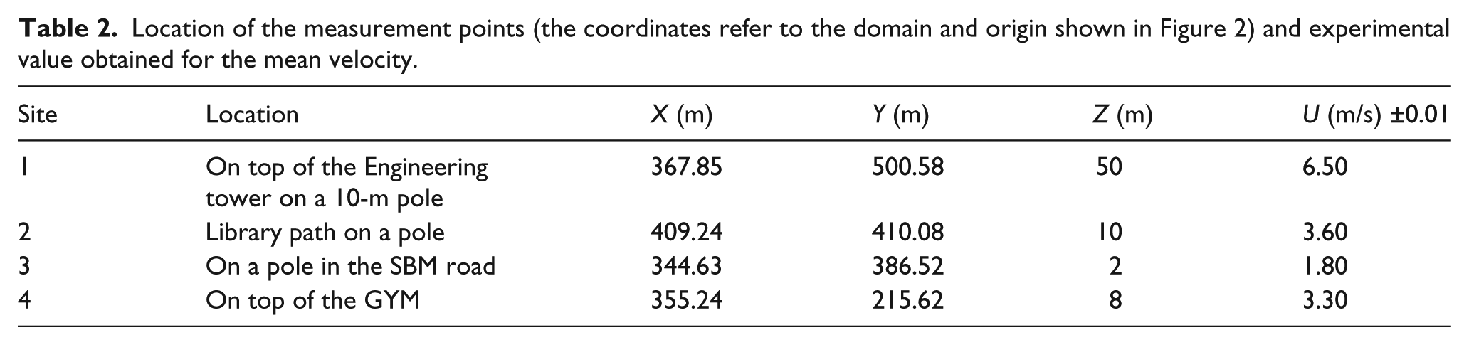
The experimental measurements were performed with cup anemometers positioned on posts at different heights around campus (see Figure 2) during the period from 15 January to 20 December 2012. Those anemometers recorded wind data every 10 s, and those data were saved in its internal data logger. The first anemometer was placed on a 10-m pole on top of the Eng tower (Site 1), the second one installed on an unused light pole near the southern part of the library (Site 2). The third anemometer was placed on a pole, in a car park (Site 3), and the last one was placed on top of the Gymnasium (Site 4). Each anemometer was placed at different heights above ground level. These sites were chosen due to their availability so as to be able to monitor the wind potential at different locations on the campus. The AWS (1997) wind resource assessment handbook was used as a guide for data filtering. It should be mentioned that the anemometers were verified and calibrated by the supplier (Barani Design Company) before being utilized for this study. For the duration of 1 year, the data were averaged over 10-min intervals and filtered in case of sensor malfunction, missing data, and other typical errors.

Figure 2.

Position of the experimental measurement sites—the southeast wind flow through the measurement points is also shown.

Apart from the experimental measurements, it is important to gain information on the type of wind activity which is present at the location and from which direction the wind is predominant, so that the reference wind velocity could be specified in the CFD model at the inlet boundaries. All these information were obtained from wind data recorded at the Vacoas Meteorological station, which is the nearest weather station. Wind measuring equipment at the weather station was located at a height of 10 m s.g.l. Hourly data are available for the same period (15 January to 20 December 2012). For CFD validation purposes, the wind velocity data were carefully analyzed in view of selecting a short period of time during which the atmospheric condition was neutrally stratified. Average wind speed of 10 min was considered, for which the mean wind velocities were computed for the different sites and are displayed in Table 2.

Table 2.

Location of the measurement points (the coordinates refer to the domain and origin shown in Figure 2) and experimental value obtained for the mean velocity.

Site	Location	X (m)	Y (m)	Z (m)	U (m/s) ±0.01
1	On top of the Engineering tower on a 10-m pole	367.85	500.58	50	6.50
2	Library path on a pole	409.24	410.08	10	3.60
3	On a pole in the SBM road	344.63	386.52	2	1.80
4	On top of the GYM	355.24	215.62	8	3.30

CFD simulation: validation and solution verification

Computational model and domain

The three-dimensional digitalization of the campus buildings was performed using AutoCAD software and Global mapper with the actual urban features taken into consideration. Figure 3 shows the domain used for the CFD simulations. The domain is defined according to the best practice guidelines (Franke et al., 2007). That is, the distance between the inlet and the buildings is 8H = 320 m (H = 40 m being the highest height of the buildings) in order to allow a realistic flow development (Bartzis et al., 2004), the distances between lateral sides and closest building are 5H = 200 m, the distance between the buildings and the outlet is 15H = 600 m, and the vertical size is 10H = 400 m. Figure 4 shows the meshes used in WindSim and OpenFOAM.

Figure 3.

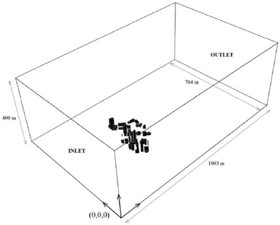
Domain used for the CFD simulations.

Figure 4.

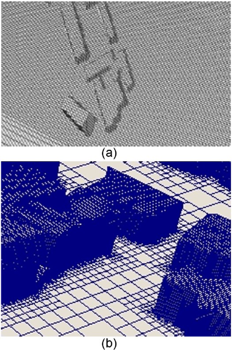
Mesh refinements used in WindSim and OpenFOAM: (a) a view of mesh used in WindSim (5 million cells), and (b) a view of Mesh refinement around the buildings used for the CFD calculations in OpenFOAM (5 million cells).

Boundary conditions

The inlet boundary conditions which are used in the simulations were based on the measured incident vertical profiles of mean wind speed. A logarithmic mean wind velocity profile representing a neutral atmospheric boundary layer according to Richards and Hoxey (1993) was imposed as follows

U (z) = \frac{U_{*}}{κ} \ln [\frac{z + z_{0}}{z_{0}}]

(10)

where z is the vertical distance from the bottom boundary of the domain and $z$ is the aerodynamic roughness length that corresponds to the site topology (in this work, $z_{0}$ is taken as 0.05 m). $U_{*}$ is the friction velocity which is obtained by including $z = z_{ref} = 10 m$ and $U_{ref} = U (z_{ref}) = 5 m / s$ in equation (10).

Richards and Hoxey (1993) further suggested that the inflow profile of the turbulent kinetic energy and dissipation rate of kinetic energy at the inlet boundary to be taken, respectively, as

k = \frac{U_{*}^{2}}{\sqrt{C_{μ}}}

(11)

and

ε (z) = \frac{U_{*}^{3}}{κ (z + z_{0})}

(12)

For both CFD codes, in the case of the ground surface, the standard wall functions by Launder and Spalding (1974) were used. Zero static pressure was applied at the outlet, and symmetry conditions were applied for the top and lateral sides of the domain as per the best practice guidelines (Franke et al., 2007). It should be noted that the mean wind velocity computed for the inlet was 5 m/s at 10 m height coming from the Southeast direction (150°). The latter wind information was integrated into the CFD models as inlet wind conditions.

Grid convergence analysis

A grid sensitivity test was performed by coarsening the reference grid with a factor of about 2. The reference grid is 5 million cells, the medium grid is 2.7 million cells, and the coarse grid is 1 million cells. The CFD wind speed results of the three grids are compared in Figure 5(a) and (b) for both OpenFOAM and WindSim, respectively, with experimental data. To check the order of convergence of the numerical scheme, the grid convergence index $(G C I)$ is calculated according to Roache (1998) using the total number of cells (N) and the hit rate (HR). Since we used three different meshes, the grid convergence index is

G C I_{21} = 1.25 \frac{(e_{21})}{r_{21}^{p} - 1}

(13)

where the relative error e₂₁ is

e_{21} = \frac{H R_{2} - H R_{1}}{H R_{1}}

(14)

Figure 5.

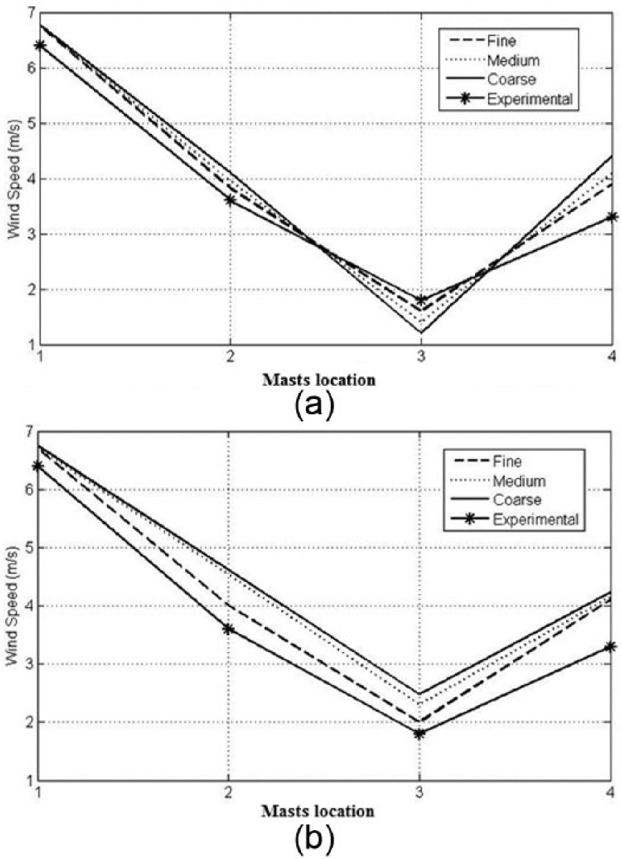
Comparison of CFD simulation results with experimental data for sensitivity analysis: (a) OpenFOAM and (b) WindSim.

The effective grid refinement, r₂₁, is given by

r_{21} = {(\frac{N_{1}}{N_{2}})}^{1 / 3}

(15)

The observed convergence rate, p, is

p = \frac{| \ln | \frac{R M S_{3} - R M S_{2}}{R M S_{2} - R M S_{1}} | + q (p) |}{\ln r_{21}}

(16)

where

q (p) = \ln (\frac{r_{21}^{p} - s}{r_{32}^{p} - s})

(17)

and

s = s n g (\frac{R M S_{3} - R M S_{2}}{R M S_{2} - R M S_{1}})

(18)

where RMS_i (i = 1, 2, 3) is the root mean square (RMS) error of grid i.

Note that the system of equations (16) and (17) must be solved by means of an iterative procedure, starting with $q = 1$ . The subscripts 1, 2, and 3 above refer to the fine, medium-size, and coarse meshes, respectively.

For the OpenFOAM simulations, the observed convergence rate is $p = 2.0$ and the grid convergence index is GCI₂₁ = 0.016 (1.6%). For the WindSim simulations, the observed convergence rate is $p = 2.09$ and the grid convergence index is GCI₂₁ = 0.030 (3%). Second-order convergence is observed in both solvers $(p \approx 2)$ , although for WindSim, the convergence rate is slightly lower than for OpenFOAM. Additionally, the error band in WindSim is further from the asymptotic value of the solution comparing with OpenFOAM $(G C I_{WindSim} > G C I_{OpenFOAM})$ .

Impact of turbulence model

The impact of the turbulence models on the simulated air flow patterns around the urban case is important when comparing two different CFD softwares. Table 3 shows a comparison of results obtained using the three turbulence models—standard k-ε, RNG k-ε, and k-ε with Yap correction—for both WindSim and OpenFOAM, with that of the experimental data obtained for the wind velocity at Sites 1–4. For both software, the best result is obtained on using the k-ε with Yap correction turbulence model which also yielded the lowest RMS error of 11.25% for OpenFOAM and 14.53% with WindSim. It is generally observed that at Site 3 (2 m a.g.l.), the relative error is generally higher for both WindSim and OpenFOAM, which can be attributed to thermal effects.

Table 3.

Comparison of the experimental data for the wind velocity (U) with the simulation results for different turbulence models for both WindSim (WS) and OpenFOAM (OF).

Site	Experimental result	Standard k-ε				RNG k-ε				Yap k-ε
	U (m/s) ±0.01	WS		OF		WS		OF		WS		OF
	U (m/s) ±0.01	U (m/s)	Rel. error (%)	U (m/s)	Rel. error (%)	U (m/s)	Rel. error (%)	U (m/s)	Rel. error (%)	U (m/s)	Rel. error (%)	U (m/s)	Rel. error (%)
1	6.50	6.00	7.69	6.75	3.85	6.00	7.69	6.79	4.46	6.70	3.08	6.75	3.85
2	3.60	4.00	11.11	3.99	10.83	4.00	11.11	3.90	8.33	4.00	11.11	3.82	6.11
3	1.80	2.30	27.78	1.39	22.78	2.40	33.33	2.00	11.11	2.00	11.11	1.60	11.11
4	3.30	3.01	8.79	3.7	12.12	3.63	10.00	4.10	24.24	4.10	24.24	3.90	18.18
RMS error (%)			16.06		14.12		18.67		14.15		14.53		11.25

RNG: renormalization group; RMS: root mean square.

Qualitative analysis

A slice of the velocity field at 10 m a.g.l. is shown in Figure 6 for both WindSim and OpenFOAM, in order to observe the wind flow patterns. From the physics point of view, it is clearly seen that there exist regions of high velocity, especially near both the MIE and MES buildings as well as at the foot of the Eng tower, which are high-rise buildings, and significantly higher than all others on the campus. Actually, these regions are regularly invaded with daily wind gusts which are felt by students whose clothes get disheveled or having their umbrella go flying. The concentration effect of the wind is observed in all the heights analyzed, and the wind velocity is particularly high on the roof of the tallest buildings.

Figure 6.

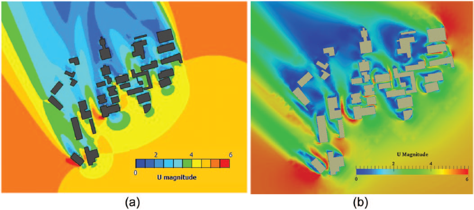
Wind velocity fields (in m/s) at 10 m height in both (a) WindSim and (b) OpenFOAM. The North is at the top, and the incident wind direction is SE.

Verification of the turbulence modeling for different incident wind directions

As stated earlier, data were measured at four fixed locations for a 1-year period. Validation required measured data from sufficiently long sampling period as stated by Schatzmann and Leitl (2011). Figure 7 compares the simulated and measured mean wind speed for both CFD software WindSim and OpenFOAM at the four locations for six reference wind directions. The figure shows a fair agreement for OpenFOAM which overall has a lower RMS error. For the case of WindSim, the results show a quite large deviation, although for some locations and directions the wind speed is quite comparable with that of OpenFOAM. For Site 2, it is observed for both WindSim and OpenFOAM that there is large deviation from the measured data. This can be attributed to the fact that due to lack of computational power, the CFD models were not fine enough at that level.

Figure 7.

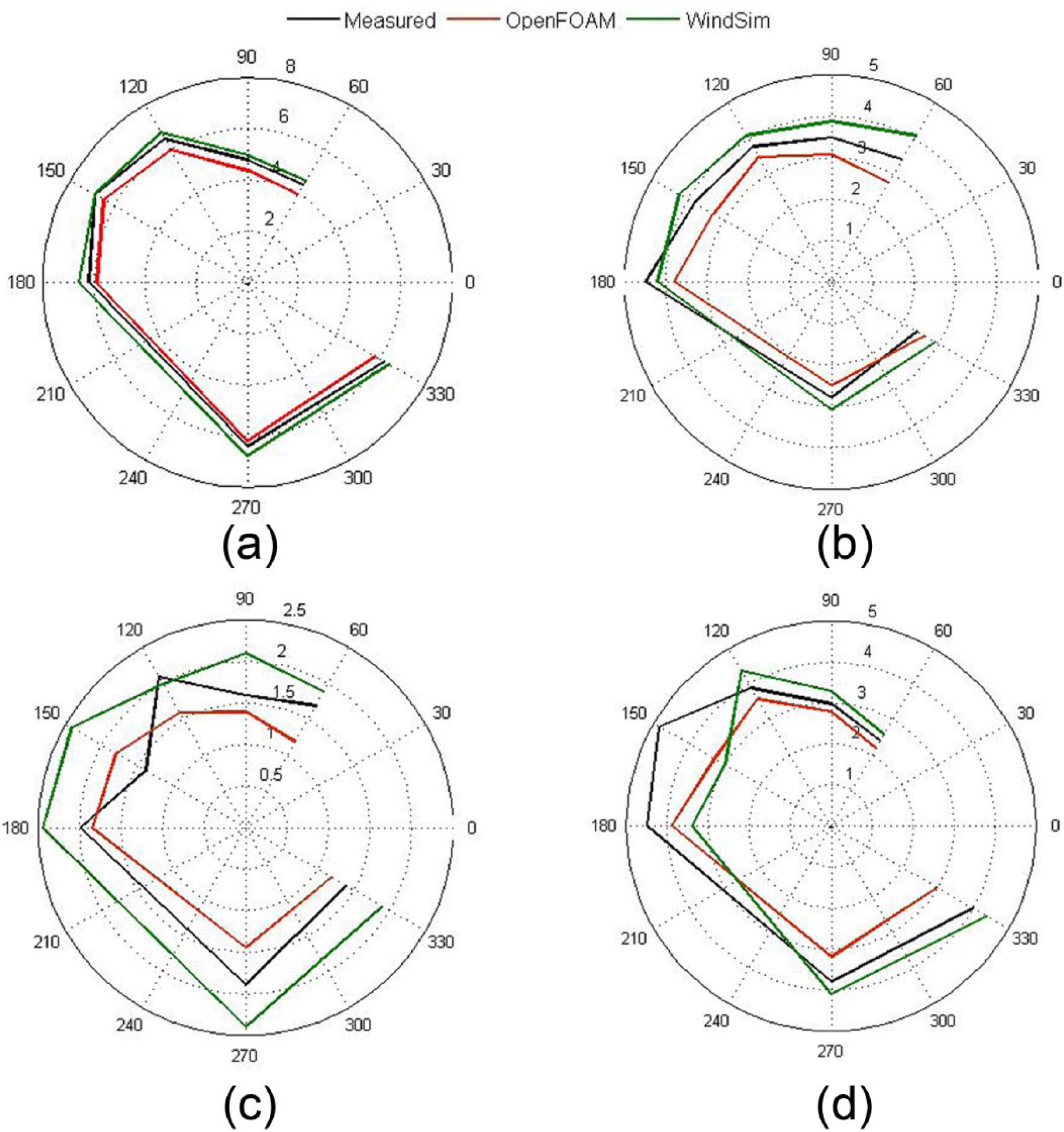
A comparison of both CFD software with measured data: (a) Site 1 at 50 m a.g.l., (b) Site 2 at 10 m a.g.l., (c) Site 3 at 2 m a.g.l., and (d) Site 4 at 8 m a.g.l.

Conclusion

This article presents a comparison of the results obtained using two different CFD solvers with the in situ measurements of wind data in a small urban area, the UoM campus. The CFD commercial software WindSim and the open source package OpenFOAM were used to simulate the wind flow pattern over the campus using three turbulence models: standard k-ε, RNG k-ε, and k-ε with Yap correction. OpenFOAM and WindSim have shown the best results for the turbulence model k-ε with Yap correction with lowest RMS errors. It is found that the accuracy of the measurement points position identification is extremely important. Additionally, the geometry of the buildings close to the measurement points has to be exhaustively reproduced in the simulations. The measurement points must be placed in areas without elements not considered in the simulation (e.g. trees, signals, cars, and parking). These aspects are the main source of divergences between experimental and simulation results in our case study. Regarding the solution verification, second-order convergence was observed in both solvers, although the error band in WindSim was further from the asymptotic value of the solution comparing with OpenFOAM. We can therefore conclude that the best results for the CFD simulation of the wind flow around buildings were obtained using OpenFOAM. Both solvers solve same RANS equations using same discretization schemes but obtained different results. This is attributed due to the fact that the grids are different; in OpenFOAM, the grids are uniform around the buildings. An important difference between the two models lies in the gridding system. The WindSim mesh is of inferior quality as the mesh generated by the OpenFOAM utilities. We have ignored unsteady effects in this investigation, which only considered steady solutions. Unsteady effects can have an effect on the results, in particular if the turbulence model is capable of capturing recirculation effects on the buildings. We have also ignored the effects of the surrounding forest canopy. A future investigation will explicitly consider the effects of the vegetation using a forest model.

Footnotes

Acknowledgements

The authors acknowledge the University of Mauritius for allowing the installation of anemometers around the campus and the Mauritius Research Council (MRC) for supporting the research work of the first author (A.Z.D.) through a postgraduate scholarship. Additionally, the authors acknowledge the computer time provided by the Facility for Large-scale Computations in Wind Energy Research (FLOW) at the University of Oldenburg and the Euler cluster at the CIEMAT. The authors further extend their thanks to Dr Nima Samkhaniani from Tarbiat Modares University for technical advices and to Razia Baboorally for her help in collecting wind data.

Declaration of conflicting interests

The author(s) declared no potential conflicts of interest with respect to the research, authorship, and/or publication of this article.

Funding

The author(s) received no financial support for the research, authorship, and/or publication of this article.

References

AWS (1997) Wind resource assessment handbook: Fundamentals for conducting a successful monitoring program. Report prepared for National Renewable Energy Laboratory. NREL Subcontract no. TAT-5-15283-01, April. Albany, NY: AWS Scientific, Inc.

Baik

Kang

Kim

(2007) Modeling reactive pollutant dispersion in an urban street canyon. Atmospheric Environment 41: 934–949.

Bartzis

Vlachogiannis

Sfetsos

(2004) Thematic area 5: Best practice advice for environmental flows. QNET-CFD Network Newsletter 2: 34–39.

Blocken

Carmeliet

(2002) Spatial and temporal distribution of driving rain on a low-rise building. Wind and Structures (5): 441–462.

Blocken

Carmeliet

(2004a) A review of wind-driven rain research in building science. Journal of Wind Engineering and Industrial Aerodynamics 92(13): 1079–1130.

Blocken

Carmeliet

(2004b) Pedestrian wind environment around buildings: Literature review and practical examples. Journal of Thermal Envelope and Building Science 28(2): 107–159.

Blocken

Carmeliet

Stathopoulos

(2007) CFD evaluation of wind speed conditions in passages between parallel buildings—effect of wall-function roughness modifications for the atmospheric boundary layer flow. Journal of Wind Engineering and Industrial Aerodynamics 95(9–11): 941–962.

Blocken

Carmeliet

Moonen

. (2008) Numerical study on the existence of the Venturi effect in passages between perpendicular buildings. Journal of Engineering Mechanics-ASCE 134(12): 1021–1028.

Britter

Hanna

(2003) Flow and dispersion in urban areas. Annual Review of Fluid Mechanics 35: 469–496.

10.

Britter

Schatzmann

(2007) Background and Justification Document to Support the Model Evaluation Guidance and Protocol, 3-00-018312-4 COST Office, Brussels, Belgium Cost Action 732.

11.

Ferziger

Peric

(2002) Computational Methods for Fluid Dynamics (3rd edn). Springer Berlin Heidelberg.

12.

Franke

Hellsten

Schlünzen

. (2007) Best practice guideline for the CFD simulation of flows in the urban environment. COST Action 732, 1 May. Brussels: COST Office.

13.

Gagliano

Nocera

Patania

. (2013) Assessment of micro-wind turbines performance in the urban environments: An aided methodology through geographical information systems. International Journal of Energy and Environmental Engineering 4: 43.

14.

GSI (2015) “Google Satellite Map,” Google Earth.

15.

Hanson

Summers

Wilson

(1986) Validation of a computer simulation of wind flow over a building model. Building and Environment 21: 97–111.

16.

Houda

Zemmouri

Hasseine

. (2012) A CFD model for simulating urban flow in complex morphological street network. The Online Journal of Science and Technology 2(1): 1–10.

17.

Kalmikov

Dupont

Dykes

. (2010) Wind power resource assessment in complex urban environments: MIT campus case study using CFD analysis. In: AWEA 2010 WINDPOWER conference, Dallas, TX, USA, 23–26 May 2010.

18.

Kang

Baik

Kim

(2008) Further studies of flow and reactive pollutant dispersion in a street canyon with bottom heating. Atmospheric Environment 42: 4964–4975.

19.

Kumar

Fennell

Britter

(2008) Effect of wind direction and speed on the dispersion of nucleation and accumulation mode particles in an urban street canyon. Science of the Total Environment 402: 82–94.

20.

Launder

Spalding

(1974) The numerical computation of turbulent flows. Computer Methods in Applied Mechanics and Engineering 3: 269–289.

21.

Liu

Leung

. (2006) Recent progress in CFD modelling of wind field and pollutant transport in street canyons. Atmospheric Environment 40: 5640–5658.

22.

McNabola

Broderick

Gill

(2009) A numerical investigation of the impact of low boundary walls on pedestrian exposure to air pollutants in urban street canyons. Science of the Total Environment 407: 760–769.

23.

Meissner

(2010) WindSim Getting Started (5th edn). Tønsberg, Norway: WindSim AS.

24.

OpenFOAM (2015) Available at: http://www.openfoam.com/ (accessed 22 July 2015).

25.

Parente

Gorlé

Van Beeck

. (2011) A comprehensive modelling approach for the neutral atmospheric boundary layer: Consistent inflow conditions, wall function and turbulence model. Boundary-Layer Meteorology 140: 411–428.

26.

Richards

Hoxey

(1993) Appropriate boundary conditions for computational wind engineering models using the k-ε turbulence model. Journal of Wind Engineering and Industrial Aerodynamics 46–47: 145–153.

27.

Roache

(1998) Verification of codes and calculations. AIAA Journal 36: 696–702.

28.

Sabatino

Buccolieri

Pulvirenti

. (2007) Simulations of pollutant dispersion within idealized urban-type geometries with CFD and integral models. Atmospheric Environment 41: 8316–8329.

29.

Sabatino

Buccolieri

Pulvirenti

. (2008) Flow and pollutant dispersion in street canyons using FLUENT and ADMS-Urban. Environmental Modeling & Assessment 13: 369–381.

30.

Schatzmann

Leitl

(2011) Issues with validation of urban flow and dispersion CFD models. Journal of Wind Engineering and Industrial Aerodynamics 99(4): 169–186.

31.

Solazzo

Vardoulakis

Cai

(2007) Evaluation of traffic-producing turbulence schemes within operating schemes within operational street pollution models using road side measurements. Atmospheric Environment 41: 5357–5370.

32.

Stathopoulos

Baskaran

(1996) Computer simulation of wind environmental conditions around buildings. Engineering Structures 18(11): 876–885.

33.

Toja-Silva

Colmenar-Santos

Castro-Gil

(2013) Urban wind energy exploitation systems: Behavior under multidirectional flow conditions—opportunities and challenges. Renewable and Sustainable Energy Reviews 24: 364–378.

34.

Toja-Silva

Peralta

Lopez-Garcia

. (2015a) On roof geometry for urban wind energy exploitation in high-rise buildings. Computation 3(2): 299–325.

35.

Toja-Silva

Peralta

Lopez-Garcia

. (2015b) Roof region dependent wind potential assessment with different RANS turbulence models. Journal of Wind Engineering and Industrial Aerodynamics 142: 258–271.

36.

Van Hooff

Blocken

(2010) On the effect of wind direction and urban surroundings on natural ventilation of a large semi-enclosed stadium. Computers & Fluids 39(7): 1146–1155.

37.

Vardoulakis

Fisher

BEA

Pericleous

. (2003) Modelling air quality in street canyons: A review. Atmospheric Environment 37: 155–182.

38.

Wesseling

. (2001) Principles of Computational Fluid Dynamics. New York: Springer-Verlag Berlin Heidelberg.

39.

Yakhot

Orszag

Thangam

. (1992) Development of turbulence models for shear flows by a double expansion technique. Physics of Fluids A-Fluid Dynamics 4(7): 1510–1520.

40.

Yap

(1987) Turbulent heat and momentum transfer in recirculating and impinging flows. PhD Thesis, Faculty of Technology, University of Manchester, Manchester, UK.