
Abstract
Wind turbines located in a wind farm are subject to a wind field that is substantially modified when compared to the ambient wind field due to wake effects. It is clear that in addition to the power, a tool that could model the loads of the waked turbine is needed. In this work, a wind farm wake model is created using a single wake model based on the dynamic wake meandering model to systematically model the wake effects and thus the power and loads of an entire wind farm with an arbitrary wind turbine layout and wind condition. This wind farm wake model is incorporated into the National Wind Technology Center design codes. Preliminary results demonstrate that this wind farm tool yields satisfactory results when compared with Simulator for Wind Farm Applications, a high fidelity computational fluid dynamics Large eddy simulation model, and with experimentally-obtained field data. The integration of the wind farm model with the National Wind Technology Center design codes is described in detail and validation results of the tool are provided.
Introduction
The ability to accurately and efficiently model wind plant performance continues to gain importance. In practice, there are a range of wake modeling methods available, which can be categorized based on the fidelity level.
High fidelity models include Large Eddy Simulation (LES) (Pope, 2000) and the Reynolds Averaged Navier–Stokes (RANS) method. These approaches require very few assumptions and the three dimensional pressure and force distribution of the wake can be directly reflected in the simulation domain. In terms of rotor representation, examples using full rotor simulations include the work of Sørensen et al. (2002) and Zahle and Sørensen (2007, 2011). The drawback of these approaches are the requirement of a very fine mesh to resolve the boundary layer and model the rotational effects of the blades, which results in substantial calculation costs. To reduce the calculation cost, the actuator line (AL) model is developed, in which the turbine is modeled as three rotating lines and the inflow impacts each blade individually. The elimination of boundary layer resolving on the blades significantly reduces the computation time and maintains accurate calculations. Examples of work using the AL model include Shen (2011), Mikkelsen (2003b), and Keck et al. (2014). Recently the National Renewable Energy Laboratory (NREL) developed the Simulator for Wind Farm Applications (SOWFA) (Churchfield and Lee, 2012), a computational fluid dynamics solver based on OpenFOAM (Open-source Field Operations and Manipulations) libraries (Openfoam, 2015) coupled with FAST (the NREL’s open-source wind turbine simulator by Jonkman and Buhl (2005)) that allows users to investigate wind plant performance under various atmospheric conditions using the AL model.
Medium fidelity models are also based on the Navier–Stokes (N–S) equations and include most of the important wake physics, but simplifying assumptions are made to reduce the complexity. For instance, the wind turbine may be represented by using the actuator disc (AD) method and the time averaged physics (Mikkelsen, 2003a). This method is often used for investigating the far-wake effects, where an acceptably accurate result is yielded, whereas the near-wake effects and the vortex structure are not included in these models. Examples of the wake applying the AD model are Steinfeld et al. (2009), Madsen et al. (2007), and Keck (2012). In addition, free wake models based on vortex segments are also commonly employed. These models use the Biot-Savart integral to model the vortex structures and the inviscid flow, thus achieving faster computation time. A more thorough review of vortex wake modeling is given by Sørensen (2011) and Vermeer et al. (2003).
Computationally efficient tools are needed for engineering design and industrial application. These models are based on reduced order physics to maintain affordable calculation cost. Due to the simplified physics, most engineering models are not applicable for estimating near-wake effects. Among the low fidelity models, the model by Jensen (1983) is the most popular one that may be used for micrositing and wind farm output predictions. The Jenson/Katic model is based on momentum conservation of the deficit in the wake caused by the wind turbine. The wake is assumed to have a uniform wind speed in the cross flow direction and the wake expands linearly and radially with downstream distance.
The goal of this paper is to introduce a recently developed, free, open-source wind farm modeling tool that provides the unique ability to model both the power performance and the aero-elastic loads simultaneously in a wind farm of arbitrary layout. This wind farm modeling tool enables a wide range of applications such as wind farm optimization, and the estimation of the combined aerodynamic, wake, and hydrodynamic loading on offshore wind turbines. Currently, most wake modeling tools are not coupled with an aero-elastic turbine solver. In this paper, the wind farm wake model is coupled to a widely used aero-elastic solver and so the aerodynamic, hydrodynamic, and structural behavior of all the turbines are inherently modeled. Moreover, by introducing a driver program, this wind farm wake model is capable of simulating a wind farm with an arbitrary turbine layout and set of external conditions.
The single wake model of the wind farm model is implemented based on the Dynamic Wake Meandering (DWM) (Larsen et al., 2008a,b, 2013; Madsen et al., 2010; Keck et al., 2012, 2013; Keck, 2015). The wind farm model is implemented in NREL’s FAST code. FAST is a wind turbine structural and system dynamics tool and is widely used in industry and academia developed by Jonkman and Buhl (2005). The combination of the two tools provides the unique capability to model an offshore wind turbine under both wake and wave effects.
Single wake model
A wake is characterized by a mean wind speed deficit and a turbulence increase behind a turbine. The wake center also moves both laterally and vertically when it marches downstream; this stochastic pattern is called wake meandering. The resulting wind field is characterized by a significantly increased turbulence intensity and a substantially modified turbulence structure.
The single wake model used in this work is based on the work presented by Larsen et al. (2008a), Larsen et al. (2008b, 2013), Madsen et al. (2010), Keck et al. (2012, 2013), Keck (2015), and is referred to as the Dynamic Wake Meandering Model (DWM). It consists of two sub-modules: (1) the quasi-steady wake deficit and (2) the downstream stochastic wake meandering process, as shown in Figure 1.
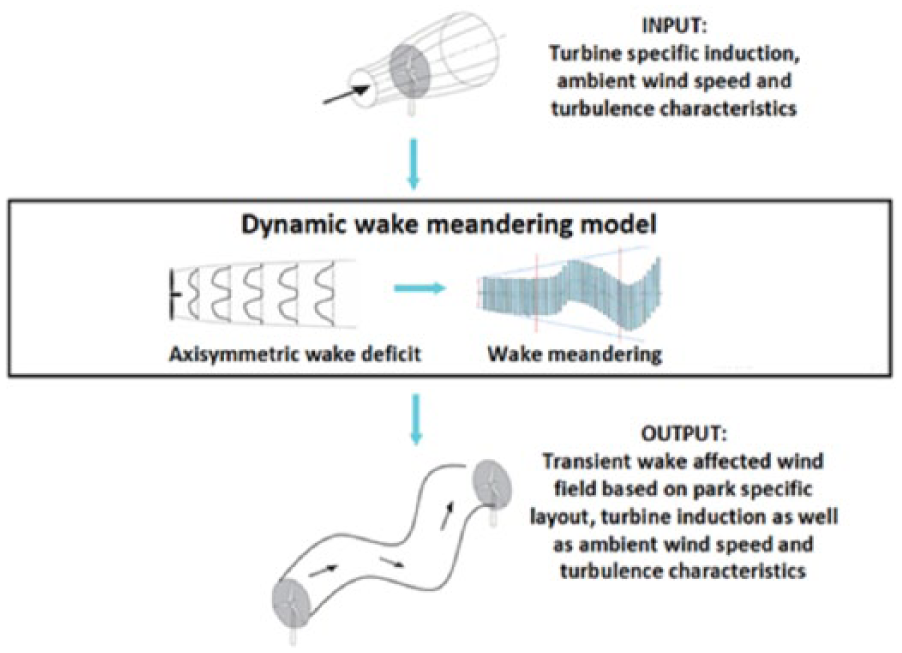
Overview of the DWM and its sub-modules (Keck et al., 2012).
Wake deficit sub-module
The implementation of wake deficit sub-model is based on the work of Keck et al. (2012, 2013), Keck (2015), in which a standalone dynamic wake meandering model is developed. DWM solves a steady state thin-shear-layer approximation of the Navier–Stokes equation. The main advantages of the standalone DWM model, compared with other current engineering models, is the ability to capture the key physics of the wake dynamics, including the turbine specific induction, the build-up of wake turbulence and the deficit in the wind farm, and the effect of ambient turbulence intensity and atmospheric stability. The drawback of the standalone DWM model is that it does not have the capability to predict turbine loads.
Therefore in this work, by implementing the standalone DWM model into the National Wind Technology Center (NWTC) design codes, waked turbine loads modeling is enabled.
With this implementation, the wake boundary condition is resolved by NWTC Information Portal (AeroDyn) (available at: https://nwtc.nrel.gov/AeroDyn), a time-domain wind turbine aerodynamics module to enable aero-elastic simulation of horizontal-axis wind turbines. A typical wake deficit profile along the span width radial locations for different downstream locations is shown in Figure 2, in which the wake recovery can be seen with the wake marches downstream.
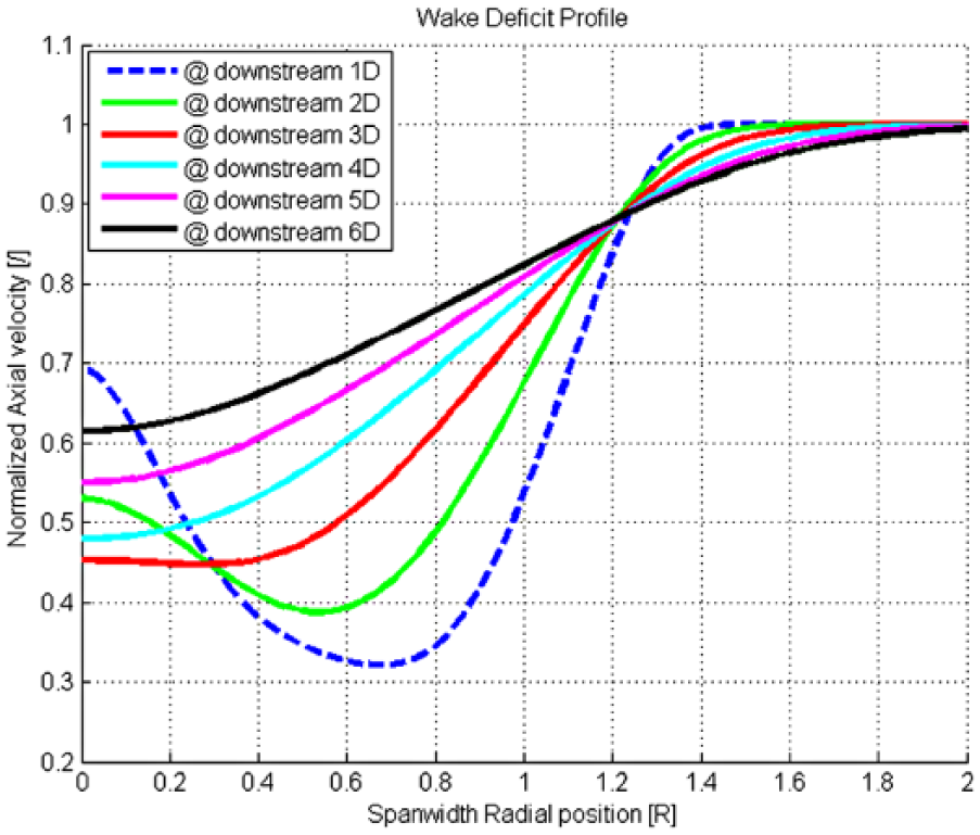
Wake deficit profile.
Wake meandering sub-module
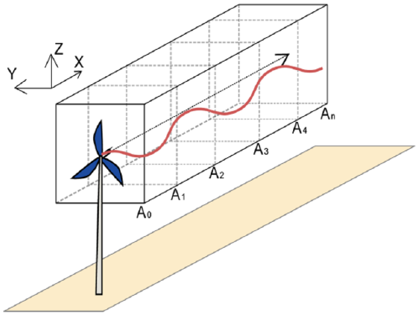
Wake meandering is the term used to describe the large-scale lateral and vertical movement of the entire wake. Wake meandering may considerably increase extreme loads and fatigue loads on turbines when the wake is swept in and out of the rotor plane. Figure 3 is a schematic of the wake meandering phenomena, where the shaded region is the general wake region behind the turbine and the multiple cross-planes represent the wake trajectory at a single time step.

Schematic of wake meandering.
The wake meandering model in this work is based on the work of Larsen et al. (2008b), which assumes that the meandering is driven by large-scale turbulent structures in the atmospheric boundary layer. Taylor’s frozen turbulence hypothesis is applied for the downstream advection of the wake. With this formulation the wake momentum in the direction of the mean flow is invariant with respect to the prescribed longitudinal wake displacement.
To determine the meandering of the wake, a turbulent inflow is first generated. Commonly, it is created by a stochastic turbulence generator, in this case NREL’s TurbSim by Kelley and Jonkman (2014), but could also be provided by LES. Then, the wake is modeled as consisting of a cascade of wake deficits, each emitted at consecutive equally spaced time increments, in agreement with the passive tracer analogy illustrated in Figure 4. The meandered wake center locations at each crossing plane
Schematic of wake meandering cascade model. The actual meandered wake center trajectory is denoted by the red curve.
Creating a wind farm wake model
Inflow wind velocity for waked turbines
In general, the wind field U can be decomposed into a mean

For a downwind turbine, the mean component in the inflow wind is not the freestream mean wind speed any more, but instead it is the wake deficit velocity calculated by the wake deficit sub-module.
The fluctuating component for the inflow wind on a waked turbine is expressed as proportional to the added turbulence intensity. The modified local wind speed to the downwind turbine

Turbulence intensity for waked turbines
Due to the wake mixing effect and the large scale meandering phenomenon, the turbulence intensity (TI) that the downstream turbines experience is no longer the same value as the leading turbine. The total turbulence intensity for the downstream turbines includes the turbulence from the wake deficit gradient (the added TI) and the wake meandering compared to the rotor fixed frame of reference (the apparent TI).
Due to the split in scales, the added turbulence intensity

Modeling multiple wakes in a wind farm
In the software implementation for modeling multiple wakes in a wind farm, turbines are first sorted from upwind to downwind according to the inflow wind direction and the turbine layout. The turbines are simulated consecutively from upwind to downwind. A downstream turbine is affected by upwind turbine(s), but not by all of them.
A pre-screening process to identity which downwind turbine is affected by which upwind turbines is required. An upwind turbine only affects a downwind turbine if the downwind turbine is located in a sector area behind the upwind turbine. The sector angle is expressed as the angle between the two edges of the wake at a certain downstream location. The lateral distance between the two edges of the wake at a certain downstream location is obtained by looping over the entire simulation time and is assigned as the maximum value of the lateral displacement of the wake edges, which guarantees the results include the contribution from both the wake expansion and wake meandering. Repeating this procedure through each downwind location yields the wake sector angle as a function of the downstream distance. The sector angles as a function of downstream distance with different TI values are shown in Figure 5.
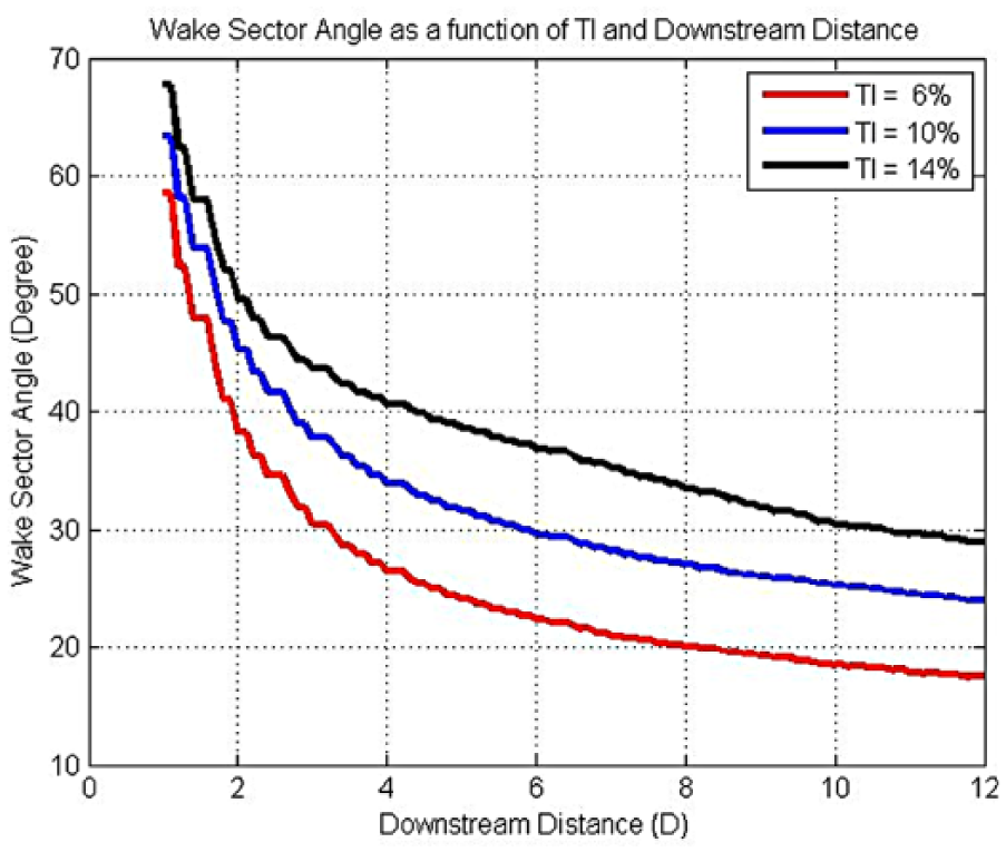
Wake sector angle as a function of TI and downstream distance.
An important issue to address when modeling wake effects deep inside a wind farm is how to handle wakes from multiple upwind turbines. In the current work, if a downwind turbine is located in a row in which there is more than one upwind turbines that affect this downwind turbine, the added turbulence intensity and the superimposed wake velocity on the waked turbine are only determined from the wake of the closest upwind turbine, or the strongest wake, for the following three reasons.
While the added TI and the superimposed wake velocity are only determined from the wake of the closest wind turbine, this does not mean that contributions from the further upwind turbines are not included. In contrast, the closest upwind turbine sees the waked flow from these further upwind turbines, which means the operating state of the closest upwind turbine is affected and altered due to the presence of those further upwind turbines.
From the work of Larsen et al. (2013), it is found that the final wake profile under multiple wakes’ interference is very similar to the closest upwind turbine’s wake for small radial locations.
The length scales involved in the meandering process are very large, whereas the length scales involved in the wake deficit formulation and recovery are very small. Due to the split of scales, it can be assumed that the wake meandering is independent on the flow disturbances from other upwind turbines.
Incorporating the wind farm wake model into the NWTC design codes
In this work, the wind farm model is incorporated within the NWTC design codes suites with the creation of a driver program, enabling the investigation of the power production and the loads variation of the turbines in the waked flow of a wind farm.
Implementing the wake model for a single turbine into FAST
The wind farm model is configured as a sub-module of AeroDyn, and when running FAST, the wind farm model is run simultaneously.
A diagram of the input/output for a single turbine is shown in Figure 6. For each turbine, the inputs of the wind farm model come from two sources—the AeroDyn loads results and the wind farm model input text files, while the outputs consist of the wake deficit velocity and the meandered wake center locations in the field behind the investigated turbines. If the turbine experiences a waked flow, a third input that includes the decreased local wind velocity and enhanced turbulence intensity from the upstream wake is added.
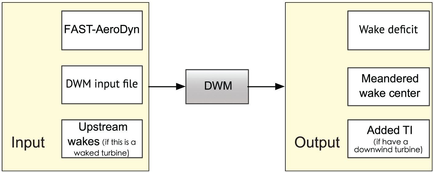
Single turbine inputs and outputs.
Seven majors steps are performed to implement the wind farm model into FAST as listed below and are presented in Figure 7.
Create the stochastic random wind field impacting the wind turbine. TurbSim generates a full 4D wind field with user defined characteristic wind speed and turbulence intensity.
Obtain the induced velocity at the rotor plane, by running a full FAST simulation with AeroDyn using the BEM method to return the time-averaged axial induction factors at each spanwise node of the blade. If the turbine does not see the freestream velocity, but instead is a downwind turbine that sees the waked flow from upwind turbines, a velocity superposition procedure is performed in the AeroDyn subroutine, in which the upstream meandered wake deficit profile is superimposed on the freestream wind as shown in equation (2).
Calculate the wake deficit field in the wake deficit sub-module.
Pass the calculated wake width at each downstream location from the wake deficit model to the wake meandering model. The wake width is used as the size of the filter, which returns the spatial averaged vertical and lateral large scale wake movement speed.
Calculate the wake meandering in the wake meandering sub-module.
If this investigated turbine’s wake affects a downwind turbine, the enhanced turbulence intensity at the downstream rotor plane with respect to the meandered wake center is calculated using equation (3) to determine the wake boundary condition for the downwind turbine.
For the next turbine, steps 2 to 6 are repeated.
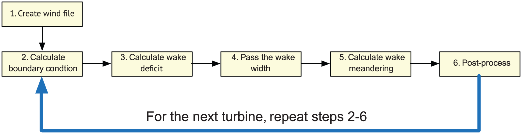
Wind farm model main steps.
Driver program and model integration
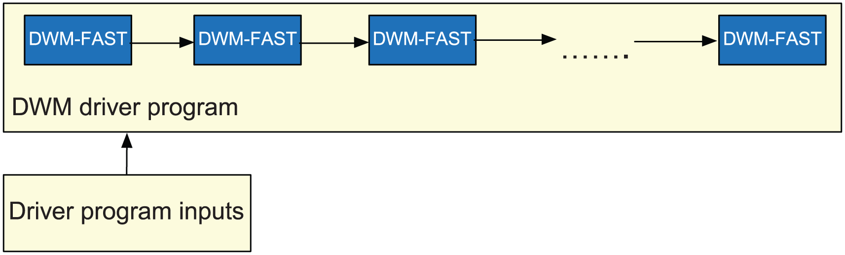
The wind farm model is implemented in FAST and the two codes are compiled together. By introducing a driver program, wind farm simulation with arbitrary turbine layout and arbitrary inflow condition is enabled. The driver program has two objectives.
The turbines are simulated separately and sequentially, so the driver program is used to manipulate the simulation of multiple consecutive independent turbines in a wind farm as shown in Figure 8.
The driver program reads in the wind farm turbine coordinate layout, the inflow wind direction and model parameters from a text input file that is similar to the FAST input file, calculates the projected distance of the wind turbine coordinates onto the inflow wind direction, and sorts/labels the turbines from upwind to downwind. The upwind wind turbines are simulated first and the downwind turbines are simulated under the influence of the upwind turbines. The sorting approaches are discussed in detail by Hao et al. (2014).
Driver program flowchart.
This wind farm wake modeling software can be downloaded for free at https://nwtc.nrel.gov/FAST8 .
Validation and results
The performance of the wind farm model is validated in terms of turbine power and loads compared with the experimentally-obtained field data and high fidelity LES results in a few wind farms.
Lillgrund wind farm
The layout of the Lillgrund wind farm is shown in Figure 9. The analysis presented here is carried out for row B (turbines 15–8) and row D (turbines 30–24). Row B contains eight turbines that have an identical spacing of 4.4D; however, the turbine that would have been the fourth turbine in row D is omitted from the actual wind farm, thus the spacing between the third and the fourth turbines is 8.8D. The ambient wind flows from the left bottom corner to the right top corner along the rows.

The layout of the Lillgrund wind farm.
The two rows in the Lillgrund wind farm are simulated with a freestream wind with a mean hub height velocity of 9 m/s and turbulence intensity of 6.2%. To minimize the uncertainties in the pregenerated wind file, five TurbSim generated wind files that have the identical wind speed and TI but different random seed numbers are applied, and the results are taken as the average value over the five cases. The Siemens SWT-2.3-93 2.3 MW turbine, with a simple torque control of
The normalized power comparison results over the two rows are shown in Figure 10. The wind farm model results are obtained directly from the AeroDyn output and compared to the OpenFOAM LES results simulated by Churchfield et al. and the field data presented by Dahlberg (Churchfield et al., 2012). At the fourth turbine in row D, where there is a larger separation from the upstream turbine, the DWM-FAST model correctly captures the wake recovery that results in the larger power production for the fourth turbine. The main deviation seen from the field data is the power production for the sixth, seventh and eighth turbine, where the OpenFOAM LES and the wind farm model both overestimate the rotor power production. This may be due to the wind direction uncertainty of the field data (Gaumond et al., 2014), boundary layer stability, deep array effect or yaw error of the turbines.
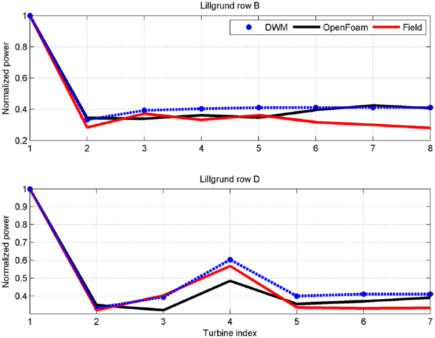
Lillgrund wind farm row B (top) and row D (bottom) power production.
OWEZ wind farm
The OWEZ wind plant, which is roughly 10 km off the shore of The Netherlands, consists of 36 Vestas V90-3.0MW wind turbines with 70 m towers as shown in Figure 11. The turbines are situated in four major rows. The turbine spacing within a row is roughly 7 rotor diameters (D) and the spacing between rows is roughly 11D. Turbines 7 and 8 are fully instrumented for mechanical loads measurements. A meteorological mast with various wind and water sensors is situated to the southwest of turbines 7 and 8.
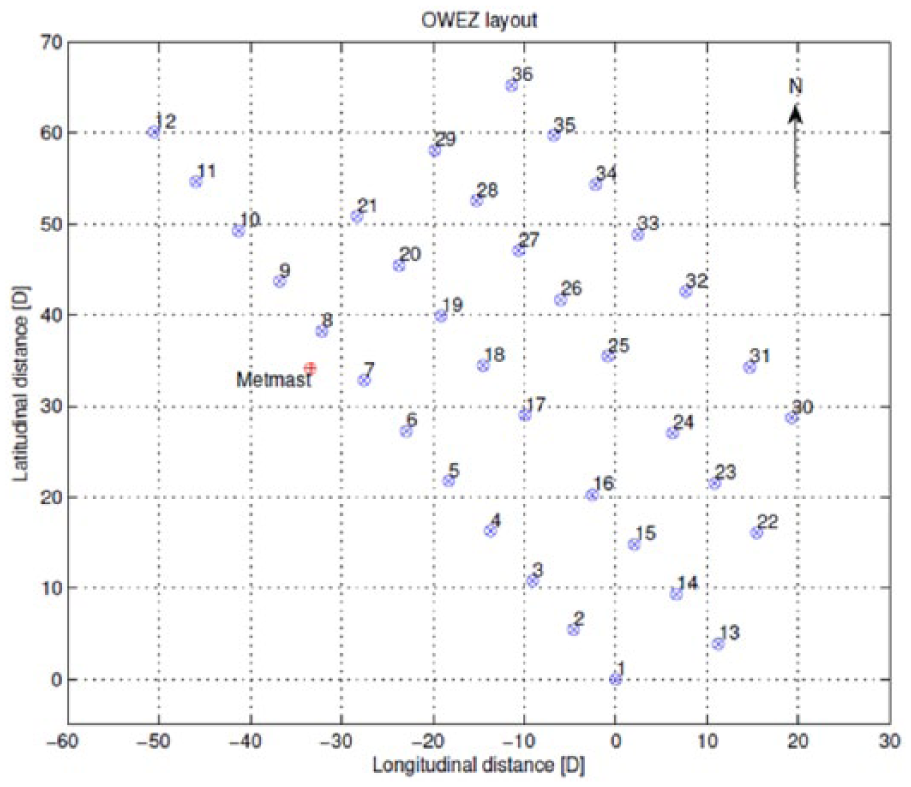
Layout of the OWEZ wind farm.
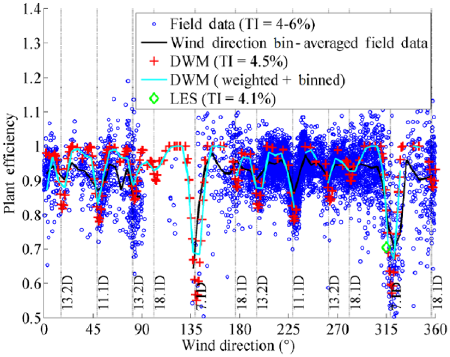
In this case, the TurbSim generated wind file has a 9 m/s hub height mean wind speed and a 4.5% turbulence intensity. In previous investigations, it is found by Gaumond et al. (2014) that wind direction uncertainty significantly impacts the wind farm modeling. Therefore, the simulation results data as a function of wind direction is convolved with a Gaussian function of wind direction centered on the wind direction of interest. For each wind direction, multiple simulations are required at and around the wind direction of interest. The convolution is done for each wind direction. The Gaussian filter is used to address the wind direction uncertainty of the field data (Gaumond et al., 2014). Because of the scatter in the field data, the Gaussian-weighted simulation data is further binned by the wind direction in order to make a useful comparison (Churchfield et al., 2015).
Figure 12 shows the wind plant efficiency versus wind direction in the 8 m/s–10 m/s wind speed bin. Wind plant efficiency is the total power generated by the wind plant divided by the power achieved if all 36 turbines were in the freestream and not subject to wake effects. Freestream power is defined as the mean of the 10-minute time-averaged power generated by the leading turbines. The blue symbols represent different data points from the field data that fit within the 8–10 m/s wind speed bin and the turbulence intensity bins. The black line is the wind-direction-bin average of these field data points within 5° bins, but portions of the line are omitted if fewer than three data samples occupy a given wind-direction bin. The red and green symbols represent the wind farm model and LES data points, respectively, with no direction-uncertainty Gaussian weighting. The cyan line is the 5° wind-direction-bin average of the Gaussian-weighted wind farm model data. The vertical black dotted lines indicated wind directions aligned with a turbine row and the turbine spacing for each of these row directions is given in terms of rotor diameters.
Plot of OWEZ wind plant efficiency versus wind direction.
From Figure 12, it can be seen that the wind farm wake model reflects the field data reasonably well and shows the ability to model the performance of an entire wind farm. Decreases in efficiency are observed when wind is aligned with rows, and the efficiency is lower for small spacings. The individual model data points lie well within the scatter of the field data.
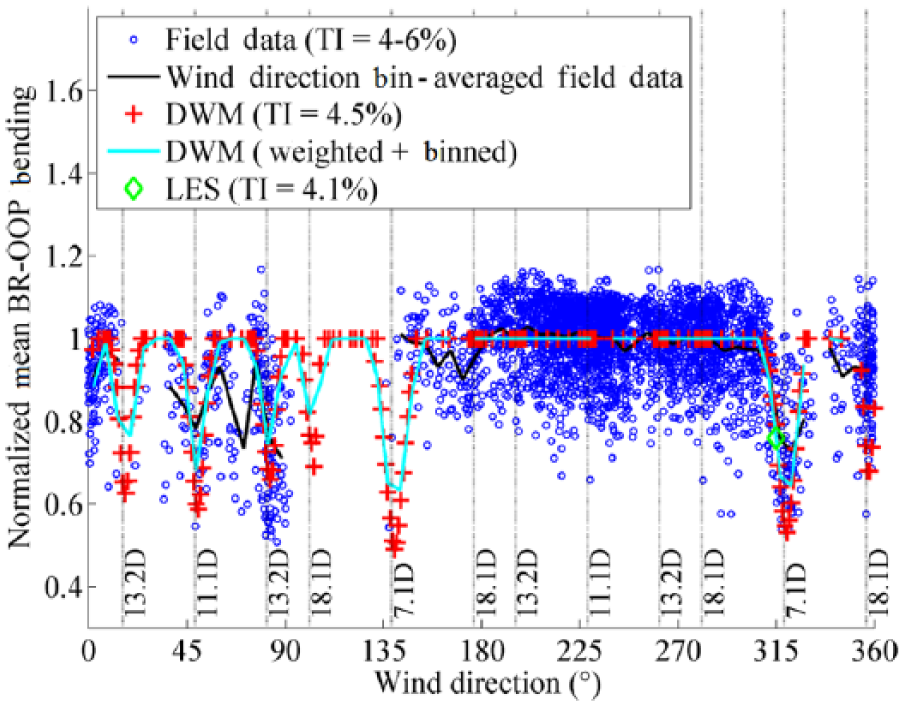
Figure 13 is the plot of turbine seven freestream normalized mean blade-root out-of-plane bending moment versus wind direction in the 8 m/s–10 m/s wind speed bin. The blade root out-of-plane (BR-OOP) is a popular choice in examining turbine structural response to its inflow because it is linked with blade fatigue. The regions of waking are clearly indicated by decreased bending moment because the rotor experiences a lower wind speed. These plots closely follow the behavior of the wind plant efficiency shown in Figure 12. For wind directions in which the turbine spacing is greater, the minimum mean BR-OOP bending moment is higher than for closer spacings, as is expected due to increased wake recovery at greater distances. More results plots and discussion are provided by Churchfield et al. (2015).
Plot of turbine 7 freestream normalized mean blade-root out-of-plane bending moment versus wind direction.
The computational cost between the LES simulation and this wind farm wake model to simulate the full OWEZ wind farm for 350 seconds are drastically different. The wind farm wake model is run on a desktop computer that is equipped with two 2.0 GHz cores and to run 100 different cases takes about 24 hours. The LES simulation is run on a high performance computing system and to run a single case requires 280,000 CPU-hrs, which is roughly six orders of magnitude different than the wind farm wake model.
Conclusion
This paper develops and introduces a wind farm wake model that systematically models both the power and loads of a wind farm with arbitrary inflow wind conditions and wind-turbine layouts. The physics of the wake modeling is based on the well-known Dynamic Wake meandering Model. By comparing the model results with experimentally-obtained field data and high fidelity LES results, it has been demonstrated that this wind farm model is capable of producing accurate results, while maintaining an acceptably low computation cost. The combination of the FAST simulation code and the wind farm model potentially provides a unique capability to model an offshore wind turbine under both wake and wave effects, and enables several other analyses, such as mooring dynamics analysis and the hydro-elastic analysis of the waked turbines, both of which were not able to be performed until this wind farm wake model was created. This software may be a useful tool for the research community, it is open-source and can be downloaded for free (Hao, 2015).
Footnotes
Acknowledgements
We would like to thank Bonnie Jonkman and Marshall Buhl for providing useful assistance in the integration of the software.
Declaration of conflicting interests
The author(s) declared no potential conflicts of interest with respect to the research, authorship, and/or publication of this article.
Funding
The author(s) disclosed receipt of the following financial support for the research, authorship, and/or publication of this article: This work was supported by the U.S. Department of Energy under Contract No. ZGV-2-22442-O1, Massachusetts Clean Energy Center and National Renewable Energy Laboratory.