
Abstract
Wind turbine power output monitoring can detect anomalies in turbine performance which have the potential to result in unexpected failure. This study examines common Supervisory Control And Data Acquisition data over a period of 20 months. It is common to have more than 150 signals acquired by Supervisory Control And Data Acquisition systems, and applying all is neither practical nor useful. Thus, to address the issue, correlation coefficients analysis has been applied in this work to reveal the most influential parameters on wind turbine active power. Then, radial basis function and multilayer perception artificial neural networks are set up, and their performance is compared in two static and dynamic states. The proposed combination of the feature selection method and the dynamic multilayer perception neural network structure has performed well with favorable prediction error levels compared to other methods. Thus, the combination may be a valuable tool for turbine power curve monitoring.
Keywords
Introduction
Continuous reductions in costs have helped to grow the size of the wind energy sector worldwide. The optimization of performance, and the management of operations and maintenance represent some of today’s largest challenges. Subsequently, numerous studies have targeted the optimization of power production, improving reliability and the general reduction of financial risk in wind farm investment (Chen et al., 2017; Gatzert and Kosub, 2016; Jia et al., 2016).
Generally, there are two principal approaches to any system performance analysis (Heng et al., 2009; Malhi et al., 2011); physics-based models can be developed (Montesano et al., 2016), or data-driven approaches can be applied (Ouyang et al., 2017; Zaher et al., 2009). The latter, which analyzes historical performance data, has a number of advantages over physics-based models. In most situations, the complexity of the machines and their sub-systems make it challenging to build accurate models. There are complex nonlinear relationships between several sub-systems of a wind turbine that make the physical modeling of the system a very complicated task to perform. The share of influence of any sub-system on the performance of other parts can be challenging to characterize. It may even differ from one turbine to another. For instance, wind farm topology, wind pattern, environmental aspects, and siting can affect machine performance in various manners (Steiner et al., 2017). In addition, the normal systems simplifications required in most physical and numerical approaches may negatively affect the results and can thus reduce the applicability of the models. Experimental methods which, can at times, be considered more valuable than numerical analysis, also suffer from major limitations. Two common challenges include the inability to identically mimic field environmental conditions in a laboratory, and the non-trivial obstacle of dynamic scaling (Giahi and Dehkordi, 2016).
Data-driven methods are well positioned for wind turbine performance analysis due to a couple of major factors: (a) A large amount of Supervisory Control And Data Acquisition (SCADA) data is available to all wind farm operators. (b) They can often be executed for less cost than comparable numerical or experimental approaches (Schlechtingen et al., 2013b; Yang and Jiang, 2011).
Data-driven studies can be categorized in two major groups. As explained by Lydia et al. (2013), the first type, a parametric model, applies a finite number of parameters to describe a distribution. For wind turbines, in particular, this type of model is established based on fitting mathematical expressions to a power curve. The other approach is known as non-parametric, in which, in contrast, the quality and quantity of parameters are not fixed in advance and are subject to change. Also in this method, the power output is a function of wind speed (Kusiak et al., 2009b).
Table 1 summarizes popular wind turbine modeling techniques, their advantages, and disadvantages. Several studies have been conducted to develop accurate data-driven models for condition monitoring of wind turbines. A comparative study using neural networks and regression-based models was conducted by Schlechtingen and Santos (2011) and Li et al. (2001), where bearing temperature was monitored in the former, while the authors in the latter performed power curve monitoring. In both studies, neural networks produced less test errors, although they were more complex in comparison with regression methods. This suggests a need for more versatile and robust models that balance comprehensiveness and simplicity of application.
Wind turbines modeling techniques comparison.

Kim et al. (2012) established two multilayer neural networks using different input signals to design a power curve–based fault detection system by way of a practical application of neural networks. A comprehensive study was conducted in Lydia et al. (2013) comparing a variety of parametric and non-parametric methods, concluding that neural networks were a reliable machine learning technique to monitor wind turbine performance.
Pelletier et al. (2016) compared multilayer neural networks with other parametric and non-parametric models and showed that their proposed neural networks resulted in less prediction error in power output. An adaptive neuro-fuzzy approach was employed by Petković et al. (2013) to estimate the power coefficient. To do so, the authors applied data obtained from the suggested equation of Heier (1998). If experimental data had been used, the results would have been more valuable. Kusiak et al. (2009a) derived nonlinear parametric models in addition to the k-nearest neighbor (k-NN) model and concluded that although the k-NN model prediction had acceptable accuracy, the parametric approach could also be used as a performance monitoring tool. Given the popularity and proven abilities of neural network modeling for turbine power analytics, they were considered for this study as well.
The work introduced in this article focuses on monitoring of wind turbine power. For this purpose, an input selection method based on the physical and statistical parameter influence on output power is introduced. Then, a dynamic neural network using historical information from inputs and outputs is constructed to estimate the power curve of the turbines. Two of the most common and powerful NN techniques (radial basis function (RBF) and multilayer perception (MLP)) are built, and their static and dynamic performance is discussed. It is shown how the feature selection method and dynamic network can generate a much more accurate model. The results are compared with existing models in the literature and it is shown that the proposed method returns the lowest prediction error. Comparisons are made in terms of mean absolute error (MAE) which is an appropriate indication of model accuracy.
The principal novelty of this article is a powerful feature selection method based on correlation analysis that enables the determination of the optimal number of inputs and outputs for comprehensive system monitoring. Furthermore, for the first time, a dynamic neural network is utilized to benefit from historical system information and improve the accuracy of the estimation.
The rest of article is organized as follows. Wind farm, turbine characteristics, and data pre-processing steps are explained in the following section. The next section after that introduces the proposed design methods consisting of the feature selection and the artificial neural networks. Then, a comprehensive simulation study and test results are provided in section “Simulation modeling and test scenario.” A detailed models comparison and analysis of the impacts of feature selection on model accuracy are also presented in this section. Finally, the last section concludes with summary of the results.
Turbine characteristics and data pre-processing
In this research, 21, 2.3 MW, pitch-regulated wind turbines have been investigated. The study takes place in a wind farm in Ontario, Canada and the data cover a range of 20 months from February 2014 to September 2015. Figure 1 illustrates the farm map and turbine layout.
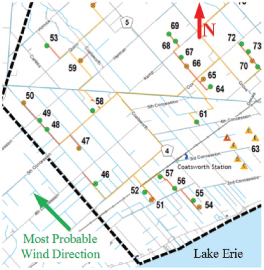
Turbine layout.
It is essential to pre-process the SCADA data before building the networks. As proposed by Schlechtingen and Santos (2011), the first step is to check the validity of data. There are two principal reasons for this. First, by omitting the extreme outliers from the data set, smoother network generalization will be easier to obtain (Swingler, 1996). Second, it is possible that due to sensor malfunction or system processing errors, the value of a parameter recorded is well out of the anticipated range as also mentioned by Caselitz and Giebhardt (2002). Thus, it is also important to carefully determine a data range to identify out-of-range values which are not results of a sensor error or misreading.
On the other hand, careful action should be taken not to eliminate anomalies that could be indicative of potential problems in machine performance. Figure 2 shows the power curve of one of the investigated turbines and extreme outliers are indicated in the figure. Since the number of these points is negligible in comparison with the whole data set and their occurrence is not regular, we assess them as anomalous and thus remove them for smoother network training.
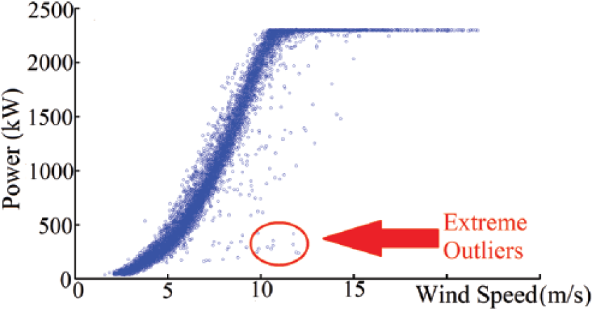
Indication of outliers in turbine power curve.
Eventually, to be able to apply the data as input parameters, the following criteria should be met (Caselitz and Giebhardt, 2002): (a) data points fall within the anticipated range, (b) components of the data set are mutually consistent, and (c) output data are consistent with the input signals.
In order to have the ability to apply multiple inputs and properly train the network, input parameters with different ranges need to be scaled to a similar range. Otherwise, the variable with wider range will dominate over others in the network training phase. Furthermore, it is normal in large data sets to have some data missing. These missing values harm the network and must be either imputed or removed depending on the application (Ching et al., 2010; Schlechtingen and Santos, 2011; Tang et al., 2015). Here, due to availability of large data, the missing values are neglected and since sampling was done at a relatively high frequency, like in Pelletier et al. (2016), 10-min average data were created and applied.
Active power translates most directly to wind farm revenue; subsequently, it was chosen as our network output signal. To monitor turbine performance, power curves that illustrate the relationship between wind speed and output power are typically applied (Pelletier et al., 2016; Taslimi-Renani et al., 2016; Wang et al., 2016). This curve, as can be observed in Figure 3, has three distinct regions. In the first region where wind speed is lower than the required minimum speed for power production, known as cut-in speed, there is no power production. In the second region, as the wind speed increases, the output power also grows rapidly until it reaches the rated power. Finally, in the third region, the power output remains constant. This region ends when the wind speed exceeds the maximum cut-out speed beyond which turbines blades are regulated to not rotate due to mechanical limitations.
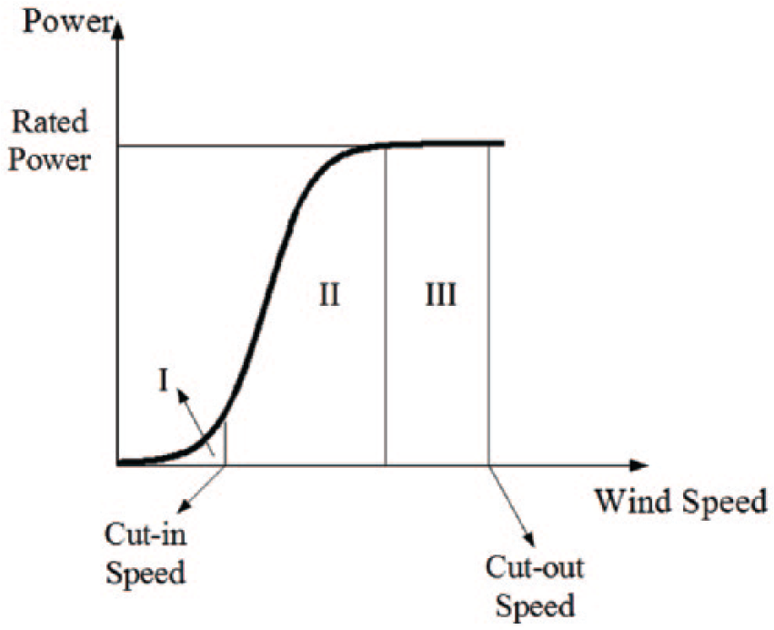
Schematic power curve of a wind turbine.
Design procedure of wind turbine monitoring
This section introduces the design methodology of the proposed monitoring method. The basic premise is to develop an intelligent estimator to fully monitor the system and track the power curve of the wind turbine using dynamic neural networks. First, the feature selection method is explained. Then, the neural network is presented.
Feature selection
A basic but crucial step in condition monitoring of any system is the appropriate selection of input and output parameters for which a number of methods have been proposed (Ghaemi and Feizi-Derakhshi, 2016; Khokhar et al., 2017; Wan et al., 2016; Wang et al., 2017). This is particularly the case for wind turbine performance monitoring, where there are many parameters available in the data and it is impractical to consider them all.
For instance, the authors in Kusiak et al. (2009b) and Li et al. (2001) used only wind speed as the input to monitor power curve. A large number of different models were developed by Schlechtingen et al. (2013b) with a variety of input-output configurations for which little specific reason was given for the selections. Sun et al. (2014) applied a genetic algorithm combined with partial least squares regression (GAPLS) method to select effective parameters to influence generator bearing temperature. It was also argued by Schlechtingen et al. (2013a) that considering environmental effects such as wind direction and ambient temperature would result in more accurate models and they considered those two parameters plus wind speed as the inputs to monitor power curve.
It is clear that the number of inputs must go beyond what is indicated by expression (1)

where
Based on equation (1), wind speed is the most influential factor on power curve modeling of wind turbines. This parameter used to be the only factor considered in many previous studies in which the power curve was modeled. Established models following this method have shown insufficient accuracy and made it clear that other parameters have to be acknowledged as well. It is proven that consideration of other relevant factors leads to more advanced models and less prediction errors. That said, indiscriminately increasing the number of inputs will decrease the neural network train-ability and result in even more errors and unreliability of the model. Finding this optimum number of values with the most influence is a challenging task.
To address this issue, we apply a statistical correlation method enhanced by knowledge of physical system. To this end, Pearson product-moment rank correlation coefficient is utilized as follows (Xu et al., 2016; Zhou et al., 2016)
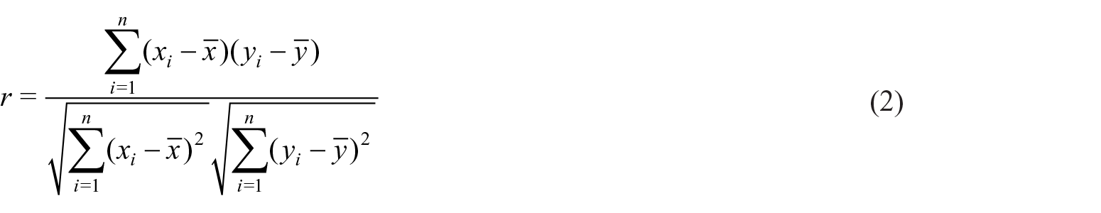
where
The artificial neural network
The MLP network is a feed-forward neural network that provides a mapping from system inputs to outputs. It is well-suited for function approximation, pattern recognition, and so on (Salahshoor et al., 2009a). The MLP consists of multiple layers of nodes in a forward direction in which each node is fully connected to the nodes in the next layer. The MLP structure is made of three types of layers including an input layer, hidden layer, and output layer. Each node in the hidden layer is a neuron with a nonlinear activation function like sigmoids, hyperbolic tangent, and so on. The input layer acts as a buffer and the output layer usually has nodes with linear functions. The MLP network applies a supervised learning algorithm known as error back propagation for training the network.
The RBF neural network is a feed-forward network that has radial basis functions as the activation function (Salahshoor et al., 2009b). The RBF Network also consists of input, hidden, and output layers. In the hidden layer, all neurons perform a Gaussian function as expressed

where
The output layer is a linear function represented as

where
Neural networks can be represented in static and dynamic structures. In the static type, the network is simply trained using the selected input parameters as described in equation (5)

where
In the proposed dynamic networks, in addition to the selected parameters as the network inputs (

Simulation modeling and test scenario
This section presents several test scenarios to validate the effectiveness of the proposed methods. In the following, the suggested feature selection method is illustrated. Then, the structure of the proposed neural network is introduced. Finally, a comprehensive comparison between proposed and existing methods and an analysis of feature selection will be provided.
The proposed feature selection for the inputs of the network
Based on the available data, physical understanding of wind turbines, and the most common parameters selected in the literature, the features to be considered as potential input signals are outlined in Table 2. Furthermore, the result of the correlation analysis given by equation (2) is also summarized in Table 2. It is indicated from this table that wind speed which is expected to have the strongest correlation with output power in comparison with other signals has the closest number to 1 with the coefficient value of 0.939.
Correlation coefficients of the selected signals.

SD: standard deviation.
While other environmental factors related to the wind, including turbulence intensity and wind direction, have been proven to have impacts on general wind turbine performance (Wagner et al., 2010), they do not appear influential for this study based on our correlations. Thus, we will not consider them to avoid increasing network complexity and training time. They may offer a marginal prediction improvement, or worse, a potentially wider range of prediction error.
Based on the results summarized in Table 2, wind speed, rotor speed, gear temperature, and blade pitch angle are selected as input parameters. Figure 4 shows a part of the input and output parameters in a high resolution time series. The correlation between parameters is visible in this figure based on their strength. Wind speed, for instance, indicates the most similar trend to power output as anticipated.
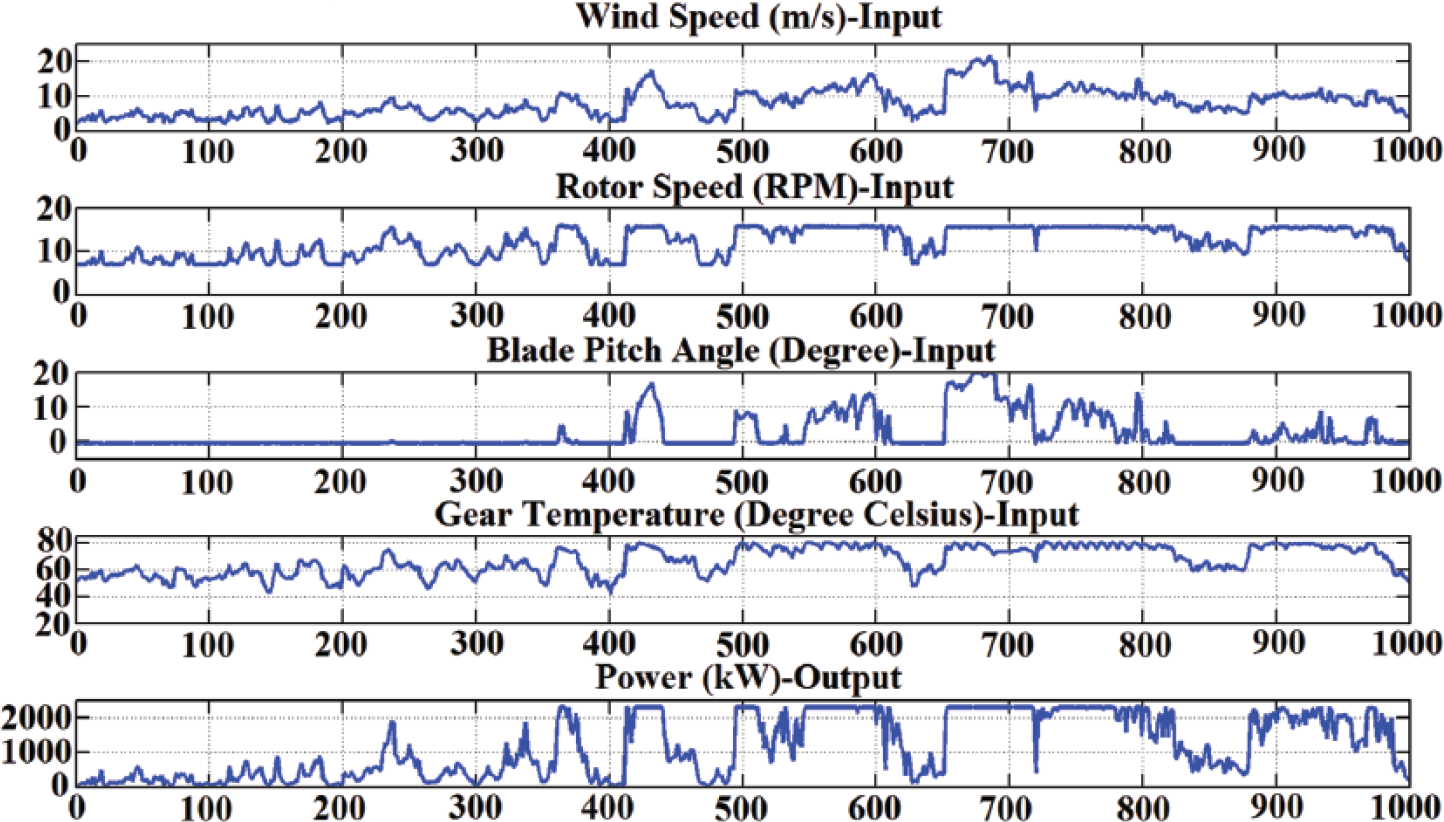
Input and output parameters.
The structure of the proposed neural networks
Static and dynamic variations of both MLP and RBF networks are established. RBF and MLP networks are established according to the structures shown in Figures 5 and 6, respectively.

RBF networks structures.

MLP networks structures.
Generally, there is no concrete rule about the size of the data complement required to obtain the best possible training, but in general, the training data should contain the data range boundaries and must be sufficient to represent the entire period (Swingler, 1996). In this study, 50% of 10-min average data was used for the training and the other half for testing. Since the data available covers all seasons, this approach makes it possible to consider seasonal changes in the network, and thus, the ambient temperature effects will be considered automatically (without it being a distinct input parameter).
To train the networks, the gradient descent with momentum method is applied. In this method, in addition to error calculation, the general error trend will also be determined. This reduces the risk of local minima and results in enhanced generalization (Schlechtingen and Santos, 2011).
The other important factor in the structure of the network is the number of neurons in the hidden layer. To be able to find the optimum number of neurons, at least 10 runs should be performed while only varying the number of neurons to seek the configuration with the best generalization (Caselitz and Giebhardt, 2002; Swingler, 1996). This helps to avoid over-fitting.
Test results are shown in Figure 7. As shown in the figure, the resulting test errors for the networks are quite acceptable. For the majority of the data points, calculated errors are in the very low range. Furthermore, it is also visible in the figures that for both MLP and RBF networks, the dynamic model outperforms the static one, based on the fact that there are more points near zero error in dynamic networks than the respective static ones.
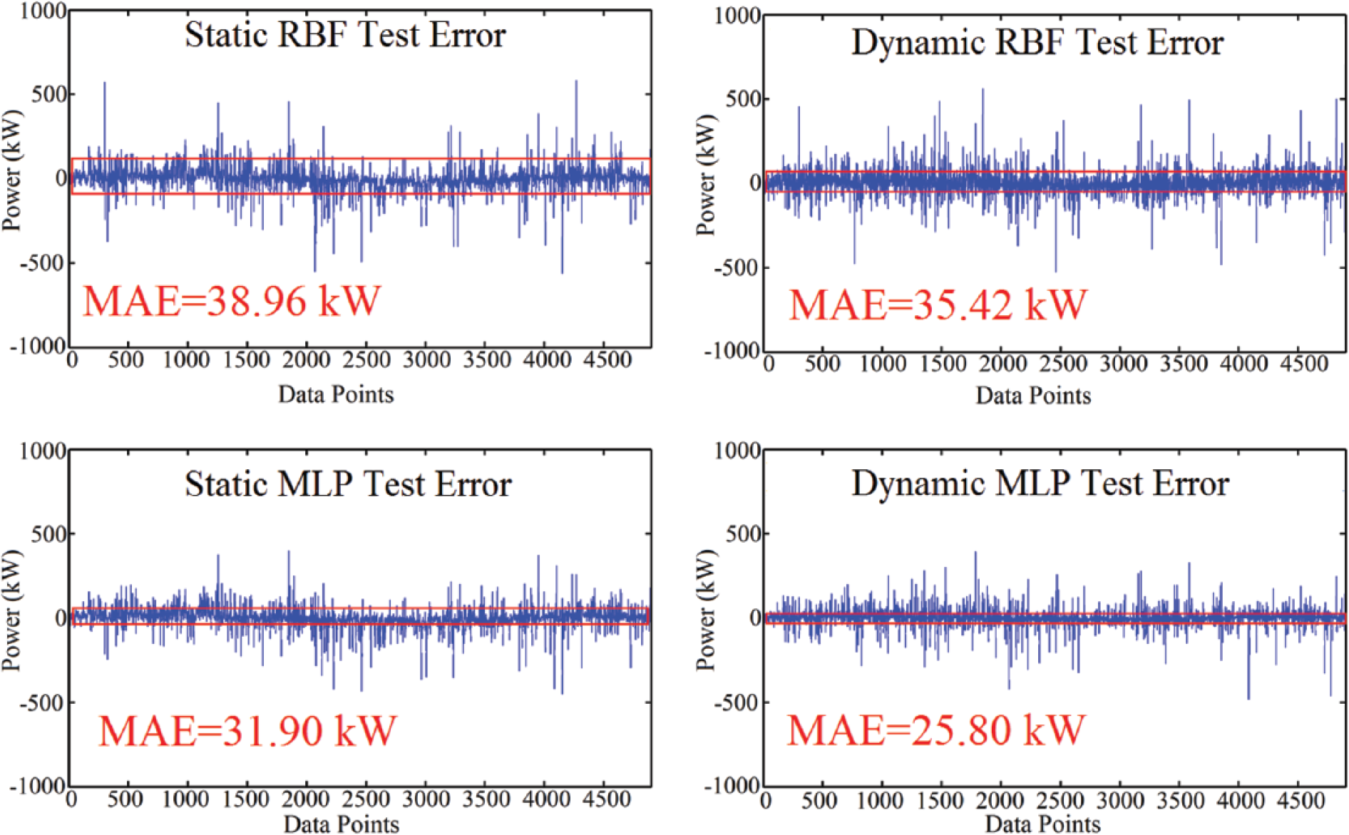
Established networks test errors.
Models comparison
MAE indicated by equation (7) has been applied to analyze the performance of the four established neural networks

where
MAE indicates the closeness of predicted results with true values. MAE is the most common type of error assessment applied in similar studies, which helps to facilitate comparison with existing models. The MAE results are summarized in Table 3. As evident in the table, the dynamic MLP network has performed the best with an MAE value of 25.80 kW. This amount of network error appears acceptable considering its magnitude relative to the 2.3 MW turbines capacity studied here. As configured, this network should reduce false alarms, increase reliability, and excel at detecting abnormal performance.
MAE results for all models.

MAE: mean absolute error; MLP: multilayer perception; RBF: radial basis function.
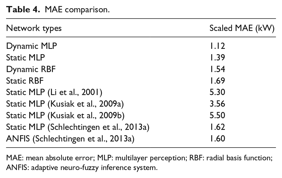
To appropriately compare the results of established models with the ones in the literature, the results should be scaled. Scaled values are presented in Table 4 along with existing models in the literature. Only NN models are considered for comparison except in Schlechtingen et al. (2013a), where models with the application of adaptive neuro-fuzzy inference system (ANFIS) has been claimed to give acceptable results.
MAE comparison.
MAE: mean absolute error; MLP: multilayer perception; RBF: radial basis function; ANFIS: adaptive neuro-fuzzy inference system.
The scaled MAE values in Li et al. (2001); Kusiak et al. (2009a, 2009b) and the two models proposed in Schlechtingen et al. (2013a) are chosen for the comparison. The authors in Pelletier et al. (2016) did not mention their investigated turbines power rating which is required for scaling. Based on the acquired results except for static RBF network, all other networks considered here outperformed those in the literature. It is also worth mentioning that the RBF network training was notably faster than MLP, an advantage in some cases.
Feature selection analysis
In order to investigate the effects of each input parameter on the MAE, in this part, MLP networks which outperformed the RBF networks are established again. First, the dynamic and static networks are trained by only wind speed, then, prediction error is calculated. In the next step, the other parameters, rotor speed, gear temperature, and blade pitch angle are added one-by-one to the networks. Results are summarized in Table 5. It is shown that by adding the appropriate input parameters, the resulting error considerably decreases, leading to better prediction performance. The dynamic MLP network, which gives the highest accuracy, has a prediction error of 42.55 kW with only wind speed as the input, and this error gradually decreases when other inputs are also included. The same trend can be observed in static model as well, confirming proper feature selection. This result seems sensible based on the role of each parameter in turbine output power. Increases in rotor speed generally suggest more power production. Gear temperature increases can be indicative of faster moving gears associated with greater power production. Finally, blade pitch angles are vital to optimizing the aerodynamics of energy capture.
Impact of each input parameter on prediction error.

MLP: multilayer perception.
Conclusion
In this article, 2.3 MW, pitch-regulated wind turbines were investigated over a period of 20 months. The output power curves were modeled using artificial neural networks. Two types of MLP and RBF networks were established in both static and dynamic states. In the dynamic configuration, the input and the output of the previous time interval were also applied to train the network. To select the most influential parameters from the data, a statistical correlation coefficient was employed. This helped enable the determination of their share of influence on the reduction of network prediction error. It was shown that by applying the rotor speed, gear temperature, and blade pitch angle, in addition to wind speed, the performance of the networks improved significantly. A 40% and 53% reduction in prediction error was observed for dynamic and static MLP networks, respectively, compared to, the state where only wind speed was considered. Furthermore, a comparison between similar models in the literature and the models proposed in this study revealed that the dynamic MLP network outperforms other models and was 30% more accurate than the best model proposed in the literature (Schlechtingen et al., 2013a). Such an outcome offers value to a growing wind energy industry that values accurate performance prediction.
Footnotes
Acknowledgements
The authors would like to thank Kruger Energy Inc. for their continued helpful support. The efforts and insights provided by Mr Jean Roy, Mr JJ Davis, and Mr Etienne Doyon are particularly noted.
Declaration of conflicting interests
The author(s) declared no potential conflicts of interest with respect to the research, authorship, and/or publication of this article.
Funding
The author(s) received no financial support for the research, authorship, and/or publication of this article.