Power curve model classification to estimate wind turbine power output

Abstract

This article presents a comparative study of empirical power curve models to estimate the output power of the turbine as a function of the wind speed. In these models, modelling strategy relies on the objective of modelling, data being used for the modelling and targeted accuracy. It has been observed that models based on presumed shape of power curve lack desired accuracy since these are developed using the power ratings of wind turbine which are not sufficient to exactly replicate the turbine’s actual behaviour. The performance of various models which comes under manufacturer power curve modelling methodology has been compared with reference to commercially available wind turbines. It has been found that power curves obtained through method of least squares and cubic spline interpolation methods exactly match with manufacturer power curve, whereas 5PL method gives sufficiently accurate results. Modelling based on actual data of wind farm has been found to be a powerful technique for developing site-specific power curves.

Keywords

Wind turbine power curve piecewise polynomial cubic spline interpolation logistic function polynomial regression

Introduction

The extraction of power from renewable resources plays an important role in addressing global energy issues. Along with solar energy, wind energy has become a recognized contributor to electricity generator. To maximize the use of wind-generated electricity when connected to the electric grid, it is necessary to estimate the power production of a wind turbine. For the feasibility of a wind energy project, accurate estimation of power production by wind turbines at future times is important. In principle, power produced $(P)$ by a wind turbine is given by Ashok (2007) and Kusiak et al. (2009)

P = C_{p} η_{m} η_{g} [\frac{1}{2} ρ A v^{3}]

(1)

Likewise, power produced by a wind turbine is proportional to many parameters such as turbine cross-sectional area A, air density ρ, wind speed v and different turbine efficiency parameters (C_p, η_m, η_g, etc.). Among all, the wind speed is the most promising factor to calculate the output of the wind turbine. In wind energy industry, a power curve helps to express the performance of turbine without giving the technical details of the components of the wind turbine generating system (Carrillo et al., 2013; Lydia et al., 2014). Wind turbine power curve determines the power produced by turbine as a function of the wind velocity. The technical specifications of the turbine are usually provided by the manufacturer in the form of nominal power curve which includes cut-in speed, rated speed and cut-off speed. Here, cut-in wind speed is the minimum wind speed at which the turbine starts to deliver useful power; rated wind speed is the speed of the wind from which the turbine starts to deliver constant maximum output power; cut-off speed is the speed at which the turbine is shut down to avoid damages from high winds. To optimize the operation cost and improve the reliability of the wind energy power system, a reliable and accurate model to estimate the power production of a wind turbine is required and limited empirical models are available for the industry to use with some boilerplate software to test the performance of the machine in actual environments.

Power curve models classification

An ideal power curve gives a typical power extraction, but it cannot be reliable for every model. Therefore, for each wind turbine, an individual power curve is required that can exhibit the characteristics of that machine only. Thapar et al. (2011) stated that commercially available wind turbines have their own design and rating because of differences in the shape of their power curves. Here, the authors have also observed that at different locations, machines having similar ratings may produce different amount of power even if the wind speed is the same. For all these reasons, modelling of the power curve is required that can reflect the actual behaviour of the machine at given site. Based on the data being used for the modelling, models can be broadly classified into three categories:

Models based on presumed shape of power curve;

Models based on actual power curve supplied by manufacturer;

Models based on actual data of wind farm.

Models based on presumed shape of power curve

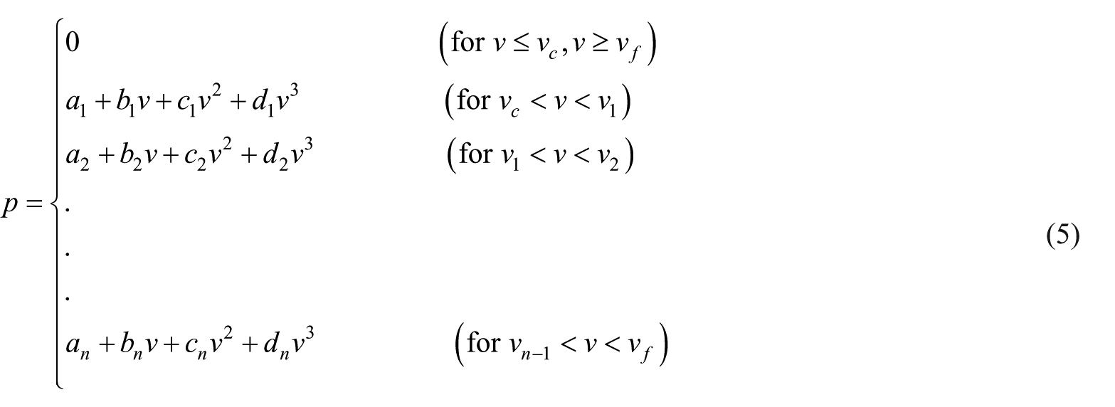
In this class, power curve of wind turbine is supposed to follow a typical shape. The power delivered by a wind turbine can be expressed by a set of characteristic equations as

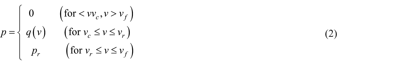
p = {\begin{matrix} 0 (for < v v_{c}, v > v_{f}) \\ q (v) (for v_{c} \leq v \leq v_{r}) \\ p_{r} (for v_{r} \leq v \leq v_{f}) \end{matrix}

(2)

These set of characteristic equations are developed using the rated power (p_r), cut-in speed (v_c), cut-off speed (v_f) and rated speed (v_r) of the selected turbine and available from the specifications of the turbine.

Modelling approaches for presumed shape power curve

Different approaches have been applied by various researchers to build a model for this class, namely: linear, quadratic, cubic and Weibull parameter-based approach. They have assumed that the relationship between output power and wind speed follows a typical relation q(v) from cut-in to rated wind speed and then it remains constant from rated to cut-off speed. Accordingly, relation q(v) has been designed by various functions using polynomial and other than polynomial expressions. Various authors have suggested different functions for the relation q(v):

Yang et al. (2003) have proposed a linear model for power estimation in which linear equation describes the relationship between output power and input wind speed. This model, though very simple, overestimates the power available.

Giorsetto and Utsurogi (1983) and Diaf et al. (2008) have presented quadratic model to describe the relation between output power and input wind speed. In this model, the relation q(v) has been designed by an equation of degree 2. This model estimates more accurately compared to simple linear model.

Chedid et al. (1998) and Nand Kishore and Fernandez (2011) have suggested a model which describes the relation q(v) by a cubic law. This model should be more realistic as ideally power of wind increases with the cube of wind speed but results are often not accurate.

Powell (1981) and Lu et al. (2002) have recommended a Weibull parameter-based model in which along with machine-specific parameters (i.e. p_r, v_c, v_f, v_r), Weibull shape parameter k has been used in the expression of power estimation. Here, the value of shape parameter k depends on wind speed distribution of selected site. Another distribution, that is, Rayleigh distribution, is a special case of Weibull distribution where the value of shape parameter is taken as k = 2, often matched with the wind profile of the selected sites (Olaofe and Folly, 2013). As a result, the expression for relation q(v) will be the same as in quadratic model. In this case, when estimating the output power of wind turbine, results are often not sufficiently accurate.

Limitations of models based on a presumed shape of power curve

It has been observed that models under this category would always lack the desired accuracy. The observation has been made on the basis of following reasons:

Model based on linear power curve does not give accurate results, as power curve of a wind turbine is seldom linear.

In these models, the characteristic equations are developed using the cut-in, cut-off and rated speeds and the rated power only which are not sufficient to exactly replicate the actual behaviour of wind turbine.

A generic polynomial curve is created between cut-in and rated speeds. Site-specific factors are not considered and machine-specific factors are considered partially. Hence, these models are not reliable for power estimation.

Models based on actual power curve supplied by manufacturer

In this class, power curve of individual wind turbine is used to develop characteristic equations using various curve fitting methods. The shape and curvature of power curves vary with different designs and rating powers. For example, there is difference between stall-regulated and pitch-regulated turbines. Stall-regulated turbines have a drop in the output power when winds get very high speed usually above the rated speed. The power delivered by a stall-regulated wind turbine can be expressed by a set of characteristic equations as

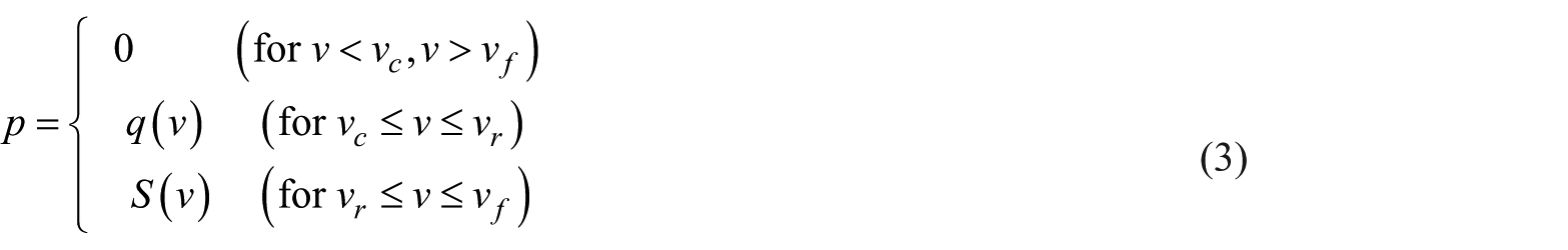
p = {\begin{matrix} 0 (for v < v_{c}, v > v_{f}) \\ q (v) (for v_{c} \leq v \leq v_{r}) \\ S (v) (for v_{r} \leq v \leq v_{f}) \end{matrix}

(3)

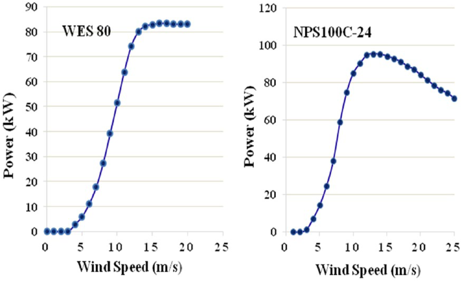
whereas pitch-regulated turbines maintain constant output power $p_{r}$ from the rated to cut-off speed. The power curves of the commercially available average rating pitch-regulated wind turbine Model no. WES 80 and stall-regulated wind turbine Model no. NPS100c-24 manufactured by Wind Energy Solutions (WES BV) and Northern Power Systems, respectively, obtained using data provided in resource file of National Renewable Energy Laboratory’s (NREL) HOMER Software (n.d.) are shown in Figure 1. While observing the different power curves as in Figure 1, it can be concluded that the typical wind turbine produces active power for wind speeds nearby 5 m/s, stops its working for wind speeds nearby 25 m/s and starts to produce maximum power for wind speeds between 12 and 18 m/s.

Figure 1.

Power curves of model WES-80 and NPS100C-24 (manufactured by Wind Energy Solutions (WES BV) and Northern Power Systems, respectively).

Modelling approaches for actual power curve

In this class, various curve fitting techniques have been used in the literature for accurately estimating the output power of that wind turbine. Since limited numbers of data points are provided by manufacturer, curve fitting using function approximation methods has been used for modelling. In this approach, the set of characteristic equations are developed by approximating relation q(v) through various functions using polynomial and other than polynomial expressions. Carrillo et al. (2013) and Nand Kishore and Fernandez (2011) have applied a second-degree and a third-degree polynomial, respectively, to fit q(v). Since in both cases, the coefficients of equations were calculated using cut-in and rated wind-power reading only, results were not so good. In order to improve fitting accuracy, this work focused curve fitting using piecewise polynomial function approximation and logistic function approximation.

Piecewise polynomial function approximation

A piecewise polynomial function q(v) is obtained by dividing the domain of v into contiguous intervals and representing q by a separate polynomial in each interval. With the aim to achieve more control on the curvature of the power curve, Thapar et al. (2011) and Ai et al. (2003) have divided wind speed domain into contiguous intervals and then a separate second-degree polynomial has been applied on each region. In each region, second-degree polynomial has been applied on three points using least squares method and achieved 100% accuracy. It has been observed that continuity of the curve at knots is not considered. More generally, a kth degree piecewise polynomial with m knots should have continuous derivatives up to degree k − 1. It is claimed that cubic piecewise polynomial are the lowest-order piecewise polynomial for which the knot-discontinuity is not visible to the human eye. Accordingly, the following equations have been applied to estimate the output power of wind turbine for given wind speeds

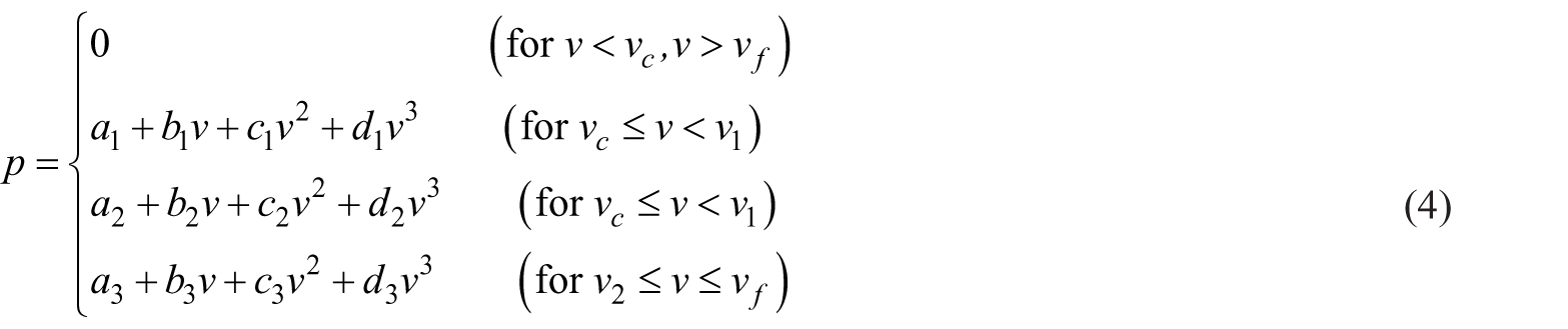
p = {\begin{cases} 0 (f o r v < v_{c}, v > v_{f}) \\ a_{1} + b_{1} v + c_{1} v^{2} + d_{1} v^{3} (f o r v_{c} \leq v < v_{1}) \\ a_{2} + b_{2} v + c_{2} v^{2} + d_{2} v^{3} (f o r v_{c} \leq v < v_{1}) \\ a_{3} + b_{3} v + c_{3} v^{2} + d_{3} v^{3} (f o r v_{2} \leq v \leq v_{f}) \end{cases}

(4)

where a₁, b₁, c₁ and d₁ are the coefficients cubic equations. Here, v₁ and v₂ are the break points also known as knots. Since a generalized model can be developed by best fitting lower degree polynomial on optimal number of data points, in experiments, knots should be selected in such a way that for fitting nth degree polynomial between knots more than n + 1 points lies in that region. As a result, it will show better accuracy on those wind speeds for which output power is not given on manufacturer power curve. Based on above approach, the power curve for model NED100, obtained from Appendix 3, equations (C.1–C.3), as compared with power curve supplied by the manufacturer is shown in left panel of Figure 2. It is observed that the empirical power curves best fit with manufacturer power curves.

Figure 2.

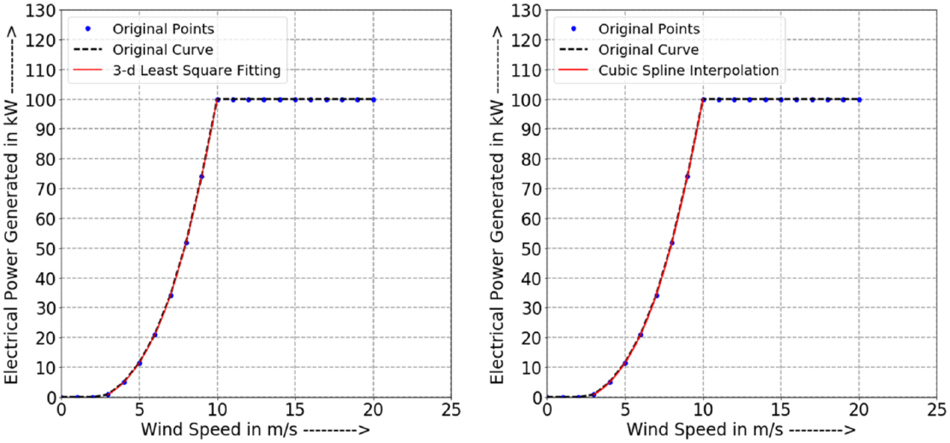
Comparison of power curves obtained from the three degree least squares and cubic spline interpolation models with the actual power curve, for model NED100 of Norvento Enerxia.

Cubic spline interpolation technique

Thapar et al. (2011) and Perera et al. (2013) have estimated the output power produced by the wind turbine through interpolation of given set of readings provided by the manufacturer. Accordingly, the following n number of cubic spline interpolation functions has applied to modelled the output power of wind turbine for given wind speeds

p = {\begin{cases} 0 (for v \leq v_{c}, v \geq v_{f}) \\ a_{1} + b_{1} v + c_{1} v^{2} + d_{1} v^{3} (for v_{c} < v < v_{1}) \\ a_{2} + b_{2} v + c_{2} v^{2} + d_{2} v^{3} (for v_{1} < v < v_{2}) \\ . \\ . \\ . \\ a_{n} + b_{n} v + c_{n} v^{2} + d_{n} v^{3} (for v_{n - 1} < v < v_{f}) \end{cases}

(5)

where a spline interpolation function of degree k is a function formed by connecting polynomial segments of degree k so that the values of function and its first k − 1 derivatives agree at the knots. In this method, the shape of a spline can be controlled by carefully choosing the number of interpolation points (or, knots) and their exact locations in order to allow flexibility and avoid overfitting where the trend changes quickly and little, respectively. Based on the above approach, the power curve for model NED100, obtained from Appendix 4, equations (D.1–D.5), as compared with power curve supplied by the manufacturer, is shown in right panel of Figure 2. It is observed that the empirical power curves best fit with manufacturer power curves.

Approximation considering inflection points of the curve

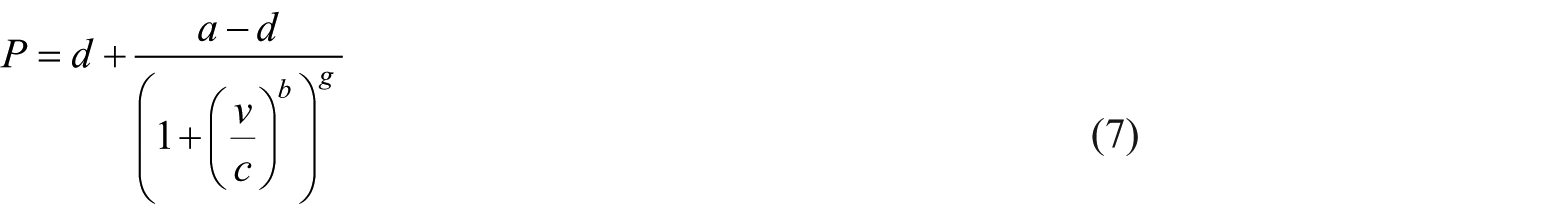
Lydia et al. (2013) have applied four-parameter logistic (4PL) function to model empirical power curve using nominal data provided by the manufacturer. They stated that in most real power curves, there is a point on the curve at which the curvature changes its sign known as inflection point of the curve. In their modelling, they have considered inflection point as one of the parameters to model the empirical power curve. The 4PL function is given below

P = d + \frac{a - d}{1 + {(\frac{v}{c})}^{b}}

(6)

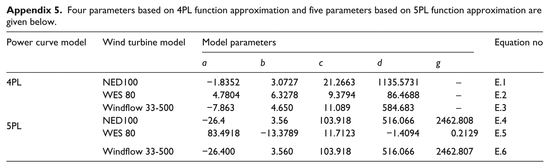
where a, b, c and d are the minimum asymptote, steepness of the curve, inflection point of the curve and the maximum asymptote, respectively, of 4PL functions. Based on the above approach, the power curve for model NED100, obtained from Appendix 5, equations (E.1–E.3), as compared with power curve supplied by the manufacturer, is shown in left panel of Figure 3. It is observed that the empirical power curves sufficiently fit with manufacturer power curves.

Figure 3.

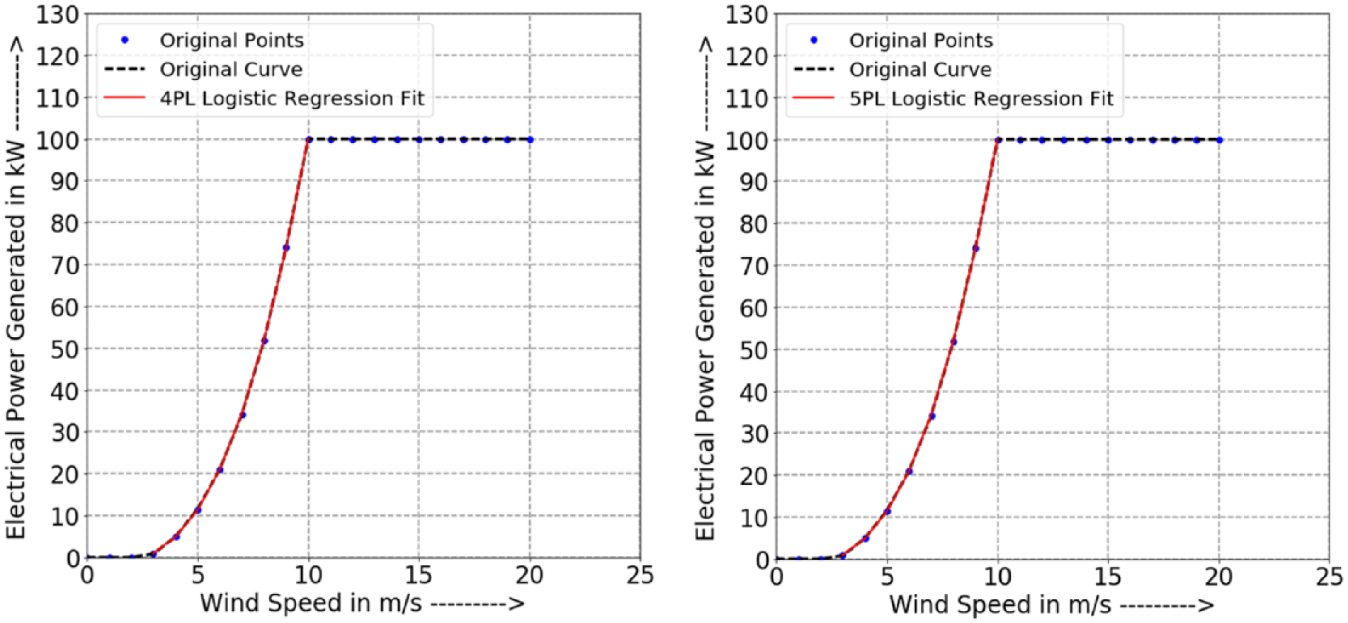
Comparison of power curves obtained from the 4PL approximation and 5PL approximation models with the actual power curve, for model NED100 of Norvento Enerxia.

More often, however, most real power curves are asymmetric about the inflection point, thus model which incorporates asymmetry factor as one of the parameters can produce better results. Sohoni et al. (2016) have applied five-parameter logistic (5PL) function to model empirical power curve using nominal data provided by the manufacturer. In their modelling, along with position of the inflection point, they have considered asymmetry factor as one of the parameters to model the empirical power curve. In this model, a typical 5PL function is given by

P = d + \frac{a - d}{{(1 + {(\frac{v}{c})}^{b})}^{g}}

(7)

where a, b, c and d parameters are same as in 4PL functions and g is the asymmetry factor of the 5PL function. Based on the above approach, the power curve for model NED100, obtained from Appendix 5, equations (E.4–E.6), as compared with power curve supplied by the manufacturer, is shown in right panel of Figure 3. It is observed that the empirical power curves sufficiently fit with manufacturer power curves.

Models based on actual data of wind farm

In this class, the empirical power curve can be developed using the data collected from the operational wind farms. Usually, the data are collected from the supervisory control and data acquisition (SCADA) system of the site. In the literature, variety of modelling techniques have been invented to model the empirical power curve of a wind turbine using actual data and some of them are reported in Marvuglia and Messineo (2012) and Morshedizadeh et al. (2017). Shokrzadeh et al. (2014) have presented a technique to describe the relation between output power and input wind speed of a wind turbine using polynomial regression fit. The polynomial regression model can be considered as

p_{i} = β_{0} + \sum_{j = 1}^{m} β_{j} h_{j} (v_{i}) + ε_{i} : h_{j} (v_{i}) = v_{i}^{j}, j = 1, \dots, m

(8)

Here, for n input observations, $p_{i}$ is the output corresponding to input observation $v_{i}, i = 1, \dots, n$ . $ε_{i}$ is the estimation error corresponding to ith input observation. Function p_i is a linear basis expansion in v_i, where h_j is the basis function of expansion. $β_{j}, j = 0, . . ., m$ are the coefficients of the polynomial. Here, the aim is find out that β for which loss (i.e. difference between actual and estimated value) is minimum. In estimation, a generalized curve is required for improving the accuracy of the model. As the number of input observations increases, to maintain the accuracy of estimator, the number of basis function increases. Relative to number of observation, if model uses too many basis functions, overfitting occurs and model becomes excessively complex. In this situation, a generalized and smooth curve can be obtained by choosing optimal number of basis function.

Results and discussion

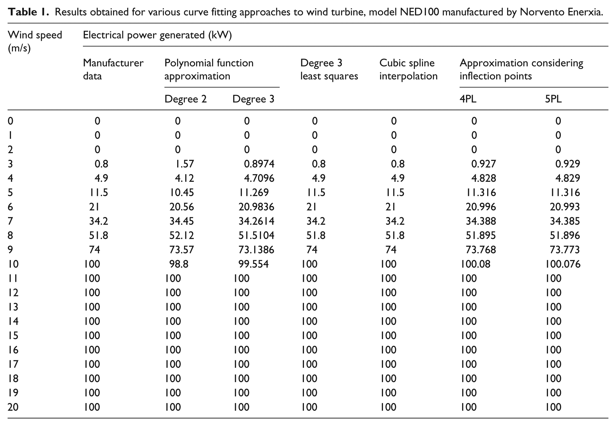
In this article, empirical power curve modelling of wind turbine has been classified into three categories. The classification is based on the wind power data being utilized for the modelling. The model based on presumed shape of power curve comes under first category and has been discussed in section ‘Models based on presumed shape of power curve’. In this class, only cut-in, cut-off, and rated speeds and the rated power are used to develop the model, which are not sufficient to exactly replicate the actual behaviour of wind turbine. In contrast, the model based on actual power curve supplied by manufacturer uses manufacturer provided nominal wind-power readings between cut-in and cut-off speeds to develop the model, resulting in improvement in estimation accuracy. The various modelling techniques representing this class, that is, polynomial function approximation, piecewise polynomial function approximation, cubic spline interpolation technique and approximation considering inflection points of the curve, have been discussed in section ‘Models based on actual power curve supplied by manufacturer’. Based on all these approaches, equations describing empirical power curves for three wind turbines, namely: NED100, WES 80 and Windflow 33-500 manufactured by Norvento Enerxia, Wind Energy Solutions (WES BV) and Windflow Technology Ltd, are shown in Appendices 1 –5. The response of each technique for NED100, WES 80 and Windflow 33-500 is demonstrated in Tables 1 to 3, respectively. As seen from Tables 1 to 3,

Table 1.

Results obtained for various curve fitting approaches to wind turbine, model NED100 manufactured by Norvento Enerxia.

Wind speed (m/s)	Electrical power generated (kW)
	Manufacturer data	Polynomial function approximation		Degree 3 least squares	Cubic spline interpolation	Approximation considering inflection points
	Manufacturer data	Degree 2	Degree 3	Degree 3 least squares	Cubic spline interpolation	4PL	5PL
0	0	0	0	0	0	0	0
1	0	0	0	0	0	0	0
2	0	0	0	0	0	0	0
3	0.8	1.57	0.8974	0.8	0.8	0.927	0.929
4	4.9	4.12	4.7096	4.9	4.9	4.828	4.829
5	11.5	10.45	11.269	11.5	11.5	11.316	11.316
6	21	20.56	20.9836	21	21	20.996	20.993
7	34.2	34.45	34.2614	34.2	34.2	34.388	34.385
8	51.8	52.12	51.5104	51.8	51.8	51.895	51.896
9	74	73.57	73.1386	74	74	73.768	73.773
10	100	98.8	99.554	100	100	100.08	100.076
11	100	100	100	100	100	100	100
12	100	100	100	100	100	100	100
13	100	100	100	100	100	100	100
14	100	100	100	100	100	100	100
15	100	100	100	100	100	100	100
16	100	100	100	100	100	100	100
17	100	100	100	100	100	100	100
18	100	100	100	100	100	100	100
19	100	100	100	100	100	100	100
20	100	100	100	100	100	100	100

Table 2.

Results obtained for various curve fitting approaches to wind turbine, model WES 80 manufactured by Wind Energy Solutions (WES BV).

Wind speed (m/s)	Electrical power generated (kW)
	Manufacturer data	Polynomial function approximation		Degree 3 least squares	Cubic spline interpolation	Approximation considering inflection points
	Manufacturer data	Degree 2	Degree 3	Degree 3 least squares	Cubic spline interpolation	4PL	5PL
0	0	0	0	0	0	0	0
1	0	0	0	0	0	0	0
2	0	0	0	0	0	0	0
3	0	0	0	0	0	0	0
4	2.9	−8.100	0.992	2.9	2.9	5.150	2.570
5	6	4.200	5.491	6	6	6.277	6.105
6	11	15.660	12.149	11	11	9.345	11.222
7	17.7	26.280	20.465	17.7	17.7	15.864	18.182
8	27.3	36.060	29.941	27.3	27.3	26.644	27.219
9	39.2	45.000	40.076	39.2	39.2	40.318	38.435
10	51.4	53.100	50.37	51.4	51.4	53.792	51.418
11	63.8	60.360	60.323	63.8	63.8	64.636	64.371
12	74.2	66.780	69.436	74.2	74.2	72.273	74.207
13	79.9	72.360	77.208	79.9	79.9	77.280	79.584
14	82.2	77.100	83.141	82.2	82.2	80.467	81.917
15	82.9	81.000	86.733	82.9	82.9	82.486	82.846
16	83.3	84.060	87.486	83.3	83.3	83.777	83.216
17	83.3	86.280	84.898	83.3	83.3	84.615	83.368
18	83	87.660	78.472	83	83	85.169	83.434
19	83	83	83	83	83	83	83
20	83	83	83	83	83	83	83

Table 3.

Results obtained for various curve fitting approaches to wind turbine, model Windflow 33-500 manufactured by Windflow Technology Ltd.

Wind speed (m/s)	Electrical power generated (kW)
	Manufacturer data	Polynomial function approximation		Degree 3 least squares	Cubic spline interpolation	Approximation considering inflection points
	Manufacturer data	Degree 2	Degree 3	Degree 3 least squares	Cubic spline interpolation	4PL	5PL
5.5	0	−27.8345	8.0065	−0.3080	−1.0637	14.0164	10.4840
6.0	20	3.4120	20.4448	20.6048	20.3376	24.3363	23.2465
6.5	41	34.0395	36.5333	41.4883	41.4828	37.7400	38.5975
7.0	63	64.0480	55.8654	62.6299	62.7133	54.5288	56.6442
7.5	85	93.4375	78.0344	84.3172	84.3703	74.8372	77.4119
8.0	107	122.2080	102.6336	106.8376	106.7952	98.5851	100.8294
8.5	130	150.3595	129.2564	130.4786	130.3293	125.4538	126.7195
9.0	155	177.8920	157.4962	155.5277	155.3139	154.8972	154.7936
9.5	182	204.8055	186.9463	182.2723	182.0904	186.1882	184.6543
10.0	211	231.1000	217.2000	211.0000	211.0000	218.4940	215.8048
10.5	243	256.7755	247.8507	241.9982	242.3841	250.9638	247.6679
11.0	275	281.8320	278.4918	275.5543	276.5841	282.8107	279.6120
11.5	308	306.2695	308.7166	309.7841	308.4298	313.3735	310.9844
12.0	340	330.0880	338.1184	342.0936	340.9872	342.1508	341.1486
12.5	371	353.2875	366.2906	371.6969	370.7578	368.8088	369.5220
13.0	396	375.8680	392.8266	398.4978	397.6553	393.1679	395.6119
13.5	422	397.8295	417.3197	422.4002	421.5933	415.1773	419.0432
14.0	443	419.1720	439.3632	443.3080	442.4856	434.8843	439.5782
14.5	462	439.8955	458.5505	461.1250	460.2458	452.4043	457.1227
15.0	474	460.0000	474.4750	475.7550	474.7875	467.8954	471.7207
15.5	485	479.4855	486.7300	487.1019	486.0245	481.5375	483.5372
16.0	492	498.3520	494.9088	495.0696	493.8704	493.5173	492.8320
16.5	498	516.5995	498.6048	499.5619	498.2389	504.0181	499.9288
17.0	500	534.2280	497.4114	500.4826	499.0437	513.2130	505.1819
18.0	500	500	500	500	500	500	500
20.0	500	500	500	500	500	500	500
25.0	500	500	500	500	500	500	500
30.0	500	500	500	500	500	500	500

Second-degree polynomial approximation does not give accurate results. However, three-degree polynomial approximation improves accuracy but again it is not enough.

While considering four points in each interval, the results obtained from method of three-degree least squares and cubic spline interpolation exactly match with manufacturer data. In contrast, as the interval size increases, the model performance slightly decreases. Overall, three-degree least squares and cubic spline interpolation outperform compared to other modelling techniques.

The empirical power curve obtained from 4PL and 5PL approximation shows less estimation error than the methods based on second- and third-degree polynomial approximation.

For all practical purpose, results obtained using 5PL approximation estimate more accurately as compared to 4 PL approximations.

Justifications for the above findings are as follows:

As the degree of fitted polynomial increases, that is, fit the data harder, model error in terms of goodness of fit to data tends to decreases. However, with too much fitting, the model generalizes poorly.

nth degree polynomial function fitting to n + 1 data points always gives exact solution.

5PL approximation produces better results than 4PL approximation, as the power curves are asymmetric and only 5PL approximation technique incorporates asymmetry factor in model parameters.

More generally, in models discussed under sections ‘Models based on presumed shape of power curve’ and ‘Models based on actual power curve supplied by manufacturer’, the characteristic equations are developed using the machine reading provided by manufacturer at fixed interval of points but again the behaviour of the machine at different site conditions are not considered. The number of readings provided by the manufacturer is limited and not sufficient to replicate the actual behaviour of wind turbine. In view of above limitations, researches have proposed power curve modelling based on actual data of operation wind farm which has been discussed in section ‘Models based on actual data of wind farm’. In this class, as in equation (8), polynomial regression has been used to estimate the relationship between turbine power output and input wind speed. This relationship helps to understand how the value of output power changes with change in input wind speed. There are many different methods to estimate polynomial coefficients, but by far the most popular is the method of least squares (Shokrzadeh et al., 2014) which focuses on goodness of fit of this function on observational data. In this approach, coefficients have been estimated by minimizing the residual sum of squares. Overall, models based on actual data of wind farm have proved to be much more successful in power curve modelling of wind turbines, where machine-specific conditions as well as site-specific conditions are considered in modelling approaches.

Conclusion

Nominal wind power readings provided by manufacturer are not sufficient to replicate the turbine’s actual behaviour. This article presented a comparative study of different empirical power curve models used for estimating the output power of the turbine as a function of the wind speed. The performance of various models are analyzed with reference to power curves of the commercially available wind turbine, obtained using data provided in resource file of NREL HOMER software. In presumed shape of power curve modelling methodology, characteristic equations are developed using turbine’s power ratings only and not suggested for the systems where accurate results are required. In modelling methods based on actual power curve supplied by manufacturer, a turbine-specific power curve is developed using the machine reading provided by manufacturer at fixed interval of points. These models showed sufficient accuracy under standard test conditions. Finally, to test the performance of wind turbine at different sites, site-specific model of power curve has been developed using actual data of wind farms. After several studies (Lee et al., 2015; Long et al., 2015; Wadhvani et al., 2017), it has been found that the wind turbine may produce different amount of power even if the wind speed is the same. In estimation, this type of predicament makes estimation a difficult task. Developing nonlinear power curve to estimate wind turbine power production would be an interesting topic for future research.

Footnotes

Appendix

Appendix 5

Four parameters based on 4PL function approximation and five parameters based on 5PL function approximation are given below.

Power curve model	Wind turbine model	Model parameters					Equation no
Power curve model	Wind turbine model	a	b	c	d	g	Equation no
4PL	NED100	−1.8352	3.0727	21.2663	1135.5731	–	E.1
	WES 80	4.7804	6.3278	9.3794	86.4688	–	E.2
	Windflow 33-500	−7.863	4.650	11.089	584.683	–	E.3
5PL	NED100	−26.4	3.56	103.918	516.066	2462.808	E.4
	WES 80	83.4918	−13.3789	11.7123	−1.4094	0.2129	E.5
	Windflow 33-500	−26.400	3.560	103.918	516.066	2462.807	E.6

Declaration of conflicting interests

The author(s) declared no potential conflicts of interest with respect to the research, authorship, and/or publication of this article.

Funding

The author(s) received no financial support for the research, authorship, and/or publication of this article.

ORCID iD

Bharti Dongre

References

Yang

Shen

et al . (2003) Computer-aided design of PV/wind hybrid system. Renewable Energy 28(10): 1491–1512.

Ashok

(2007) Optimised model for community-based hybrid energy systems. Renewable Energy 32: 1155–1164.

Carrillo

Montao

AFO

Cidrás

et al . (2013) Review of power curve modelling for wind turbines. Renewable and Sustainable Energy Reviews 21: 572–581.

Chedid

Akiki

Rahman

(1998) A decision support technique for the design of hybrid solar-wind power systems. IEEE Transactions on Energy Conversion 13(1): 76–83.

Diaf

Notton

Belhamel

et al . (2008) Design and techno-economical optimization for hybrid PV/wind system under various meteorological conditions. Applied Energy 85(10): 968–987.

Giorsetto

Utsurogi

(1983) Development of a new procedure for reliability modeling of wind turbine generators. IEEE Transactions on Power Apparatus and Systems 102(1): 134–143.

HOMER Software (n.d.) Available at: www.homerenergy.com

Kusiak

Zheng

Song

(2009) On-line monitoring of power curves. Renewable Energy 34(6): 1487–1493.

Lee

Genton

et al . (2015) Power curve estimation with multivariate environmental factors for inland and offshore wind farms. Journal of the American Statistical Association 110(509): 56–67.

10.

Long

Wang

Zhang

et al . (2015) Data-driven wind turbine power generation performance monitoring. IEEE Transaction on Industrial Electronics 62(10): 6627–6635.

11.

Yang

Burnett

(2002) Investigation on wind power potential on Hong Kong Islands—An analysis of wind power and wind turbine characteristics. Renewable Energy 27: 1–12.

12.

Lydia

Selvakumar

Suresh Kumar

et al . (2013) Advanced algorithms for wind turbine power curve modeling. IEEE Transactions on Sustainable Energy 4(3): 827–835.

13.

Lydia

Suresh Kumar

Selvakumar

et al . (2014) A comprehensive review on wind turbine power curve modeling techniques. Renewable and Sustainable Energy Reviews 30: 452–460.

14.

Marvuglia

Messineo

(2012) Monitoring of wind farms’ power curves using machine learning techniques. Applied Energy 98: 574–583.

15.

Morshedizadeh

Kordestani

Carriveau

et al . (2017) Improved power curve monitoring of wind turbines. Wind engineering 41(4): 260–271.

16.

Nand Kishore

Fernandez

(2011) Reliability well-being assessment of PV-wind hybrid system using Monte Carlo simulation. In: Proceedings of the international conference on emerging trends in electrical and computer technology (ICETECT ’11), Nagercoil, India, 23–24 March, pp. 63–68. New York: IEEE.

17.

Olaofe

Folly

(2013) Wind energy analysis based on turbine and developed site power curves: A case-study of Darling City. Renewable Energy 53: 306–318.

18.

Perera

ATD

Attalage

Perera

KKCK

et al . (2013) Designing standalone hybrid energy systems minimizing initial investment, life cycle cost and pollutant emission. Energy 54: 220–230.

19.

Powell

(1981) An analytical expression for the average output power of a wind machinex. Solar Energy 26(1): 77–80.

20.

Shokrzadeh

Jozani

Bibeau

(2014) Wind turbine power curve modeling using advanced parametric and nonparametric methods. IEEE Journal of Sustainable Energy 5(4): 1262–1269.

21.

Sohoni

Gupta

Nema

(2016) A comparative analysis of wind speed probability distributions for wind power assessment of four sites. Turkish Journal of Electrical Engineering and Computer Sciences 24: 4724–4735.

22.

Thapar

Agnihotri

Krishna Sethi

(2011) Critical analysis of methods for mathematical modelling of wind turbines. Renewable Energy 36(11): 3166–3177.

23.

Wadhvani

Shukla

Gyanchandani

et al . (2017) Analysis of statistical techniques to estimate wind turbine power generation. International Journal of Computer Science and Network Security 17(2): 247–251.

24.

Yang

Burnett

(2003) Weather data and probability analysis of hybrid photovoltaic–wind power generation systems in Hong Kong. Renewable Energy 28: 1813–1824.